FLOWER, an innovative Fuzzy Lower-than-Best-Effort transport protocol

(1)

HAL Id: hal-02540333

https://hal.archives-ouvertes.fr/hal-02540333

Submitted on 10 Apr 2020

HAL is a multi-disciplinary open access

archive for the deposit and dissemination of

sci-entific research documents, whether they are

pub-lished or not. The documents may come from

teaching and research institutions in France or

abroad, or from public or private research centers.

L’archive ouverte pluridisciplinaire HAL, est

destinée au dépôt et à la diffusion de documents

scientifiques de niveau recherche, publiés ou non,

émanant des établissements d’enseignement et de

recherche français ou étrangers, des laboratoires

publics ou privés.

FLOWER, an innovative Fuzzy Lower-than-Best-Effort

transport protocol

Si Quoc Viet Trang, Emmanuel Lochin

To cite this version:

Si Quoc Viet Trang, Emmanuel Lochin. FLOWER, an innovative Fuzzy Lower-than-Best-Effort

trans-port protocol. Computer Networks, Elsevier, 2016, 110, pp.18-30. �10.1016/j.comnet.2016.09.008�.

�hal-02540333�

(2)

To link to this article:

DOI: 10.1016/j.comnet.2016.09.008

URL:

http://dx.doi.org/10.1016/j.comnet.2016.09.008

Any correspondence concerning this service should be sent to the repository

administrator:

staff-oatao@listes-diff.inp-toulouse.fr

O

pen

A

rchive

T

OULOUSE

A

rchive

O

uverte (

OATAO

)

OATAO is an open access repository that collects the work of Toulouse researchers and

makes it freely available over the web where possible.

This is an author-deposited version published in:

http://oatao.univ-toulouse.fr/

Eprints ID: 16135

To cite this version:

Trang, Si Quoc Viet and Lochin, Emmanuel FLOWER, an

Innovative Fuzzy Lower-than-Best-Effort Transport Protocol. ( In Press: 2016)

(3)

FLOWER, an Innovative Fuzzy Lower-than-Best-Effort Transport Protocol

Si Quoc Viet Tranga,b_{, Emmanuel Lochin}a,b,∗

a_Universit´_{e de Toulouse; ISAE-SUPAERO; Toulouse, France} b_T´_{eSA, Toulouse, France}

Abstract

We present a new delay-based transport protocol named FLOWER, that aims at providing a Lower-than-Best-Effort (LBE) service. The objective is to propose an alternative to the Low Extra Delay Background Transport (LEDBAT) widely deployed within the official BitTorrent client. Indeed, besides its intra-fairness problem, known as latecomer unfairness, LEDBAT can be too aggressive against TCP, making it ill suited for providing LBE services over certain networks such as constrained wireless networks. By using a fuzzy controller to modulate the sending rate, FLOWER aims to solve LEDBAT issues while fulfilling the role of a LBE protocol. FLOWER operates to a modification of the standard LEDBAT protocol implementation by replacing its proportional controller by a fuzzy controller. Thanks to this modification, our simulation results show that FLOWER can carry LBE traffic in network scenarios where LEDBAT cannot while solving the latecomer unfairness problem. The presented algorithm is simple to implement and does not require complex computation that would prevent its deployment. Finally, we show that FLOWER remains compliant when used over an AQM-based network and remains LBE while not increasing the bufferbloat.

Keywords: Congestion Control, Lower-than-Best-Effort, LEDBAT, Fuzzy Logic

1. Introduction

While standard TCP and its variants endeavor to achieve a fair share of the network bottleneck capacity between flows, the service provided by the network remains best-effort. There exists another service named Lower-than-Best-Effort (LBE) which aims at providing a second pri-ority class inside the network traffic. The rationale is to propose a service for background traffic (e.g. peer-to-peer file transfers, data backup, software updates, . . . ) or non delay sensitive signaling traffic. This kind of traffic might tolerate a high latency and should not disturb the traffic carried out by the best-effort service itself or other ser-vices that would propose advanced QoS architecture for time-constrained application such as DiffServ [1]. Today, the LBE service, also called “scavenger” service, is per-ceived as a potential solution to fetch the unused, some-times wasted capacity in public network. One of the objec-tive is, for instance, to provide a free Internet access based on this LBE principle, as illustrated by the objectives of GAIA1 _{or PAWS}2 _{project. Last but not least, the LBE}

service should not exacerbate the bufferbloat issue [2].

∗_{Corresponding author. Address: ISAE-SUPAERO, 10 avenue}

Edouard Belin, BP 54032, 31055 Toulouse Cedex 5

Part of these results has been presented at IEEE LCN 2015. Email addresses: si-quoc-viet.trang@isae.fr (Si Quoc Viet Trang), emmanuel.lochin@isae.fr (Emmanuel Lochin)

1_Global _Access _to _the _Internet _for _All

(https://sites.google.com/site/irtfgaia).

2_{Public Access WiFi Service (http://publicaccesswifi.org).}

Among the different transport protocols providing a LBE service [3], Low Extra Delay Background Transport (LEDBAT) [4] is the most used. LEDBAT is a delay-based congestion control protocol that has been standard-ized by the Internet Engineering Task Force (IETF). LED-BAT aims to exploit the remaining capacity while limiting the queuing delay around a predefined target τ , which may be set up to τ = 100 ms according to RFC 6817 [4]. Con-sequently, LEDBAT flows limits the amount of queuing delay introduced in the network and thus lower their im-pact on best-effort flows such as TCP. As an example of application, the official BitTorrent client is using LEDBAT for data transfer [4].

Despite being a widely deployed protocol, the two main LEDBAT parameters (i.e., target and gain) have been re-vealed to be complex to determine [5, 6] as their tuning highly depends on the network conditions and not dynam-ically configurable. Indeed, LEDBAT may become more aggressive than TCP in case of misconfiguration [5, 6]. As an illustration, in a recent study, the authors of [7] conclude that the LEDBAT target parameter should not be higher than 5 ms in a large bandwidth-delay product (BDP ) network. At last, the authors of [8] show that LEDBAT can greatly increase the network latency mak-ing its impact on the network not transparent anymore.

Our protocol, FLOWER (Fuzzy LOWer-than-Best-EffoRt Transport Protocol), is a promising alternative to LEDBAT. FLOWER overcomes LEDBAT shortcomings and provides an LBE service that is more transparent to the network. The principal difference with LEDBAT is

(4)

that FLOWER replaces the linear P-type controller (pro-portional controller) of LEDBAT by a fuzzy controller to modulate the congestion window. Compared to a recent solution named fLEDBAT [9] that proposes to solve the latecomer issue and to the best of our knowledge, there is no universal scheme allowing intra-fair LEDBAT flows to remain LBE compliant, that is, non-aggressive when competing with TCP flows.

We first review in Section II the LEDBAT algorithm and its problems that motivate our work. Section III de-tails the design of FLOWER, while Section IV clearly ex-plains its core component, that is the fuzzy controller. Sec-tion V evaluates our new protocol and gives a side-by-side comparison with LEDBAT using the network simulator ns-2.35. We also demonstrated that FLOWER is more LBE-compliant than LEDBAT in the presence of AQM schemes in Section VI. We finally conclude our work in Section VII.

2. Contextual background and motivation

While many transport protocols that have been de-signed to carry LBE traffic, such as NICE [10] or TCP-LP [11], only LEDBAT has been reported to be actually deployed [12]. Our work therefore focus on LEDBAT and its design issues that are described in this section. 2.1. LEDBAT in a nutshell

LEDBAT congestion control is based on queuing de-lay variations (i.e., the queuing dede-lay is used as a primary congestion notification). LEDBAT is characterized by sev-eral parameters: target queuing delay τ , gain γ, minimum one-way delay owdmin(also called base delay), and current

one-way delay owdack. The target queuing delay τ

embod-ies the maximum queuing time that a LEDBAT connec-tion is allowed to introduce in the network. The gain γ corresponds to the reactivity of LEDBAT to queuing de-lay variations. The bigger γ is, the faster LEDBAT con-gestion control increases or decreases its concon-gestion win-dow. LEDBAT infers the queuing delay q by calculating (owdack−owdmin) obtained from one-way delays measured

by exploiting the ongoing data transfer. To keep the queu-ing delay around the predefined target, LEDBAT uses a linear P-type controller to modulate the congestion win-dow according to the derived queuing delay. For each ACK received at discrete time k, the new congestion window size cwnd is updated as follows:

∆cwnd(k) = γ(τ − (owdack(k) − owdmin(k)))

cwnd(k − 1) (1)

cwnd(k) = cwnd(k − 1) + ∆cwnd(k) (2) where ∆cwnd(k) is the change of the congestion window size.

2.2. Two main LEDBAT issues 2.2.1. Aggressiveness of LEDBAT

RFC 6817 [4] states that, if a compromised target is set to infinity, “the algorithm is fundamentally limited in the worst case to be as aggressive as standard TCP”. Ac-tually, it corresponds to the case where the buffer size is too small in comparison to the target. Thus, the queuing delay sensed by LEDBAT never reaches the target. There-fore, LEDBAT always increases its sending rate until a loss event is reported.

However, there are circumstances “worse than the worst case mentioned in RFC 6817” in which hostile LEDBAT makes TCP back off, even in an unfavorable situation for LEDBAT when it starts after TCP. The issue occurs when the buffer size is around the target. In this case, LED-BAT does not have enough time to react to queuing delay before TCP causes a buffer overflow. After that, TCP halves its congestion window, resulting in a reduction of the queuing delay. Since the queuing delay is now below the target, LEDBAT raises again its congestion window conjointly with TCP. Consequently, after several cycles, LEDBAT exploits more capacity than TCP.

To illustrate why the problem is important and the impact of the aggressiveness of LEDBAT on TCP flows, Fig. 1a shows an ns-2 simulation of 5 TCP NewReno and 5 LEDBAT flows sharing the same bottleneck with a capac-ity of 10 Mb/s. The buffer size is 84 packets (about 100 ms of delay) and the LEDBAT target is set to 100 ms. The re-sult is unequivocal and demonstrates the aggressiveness of LEDBAT flows against TCP flows. Although we present measurements with TCP NewReno, the problem remains the same with Cubic as shown later in the paper.

2.2.2. Latecomer unfairness

When LEDBAT flows start at different times, they may suffer from the latecomer unfairness problem. This prob-lem arises because latecomer flows may sense different min-imum one-way delays. In the worst case, when the buffer size is large enough, latecomer flows can starve ongoing flows.

Fig. 1b demonstrates the latecomer unfairness prob-lem. In this case, three LEDBAT flows start consecutively every 50 s and share the same bottleneck with a capacity of 10 Mb/s. The buffer size is 167 packets (about 200 ms of delay). The LEDBAT target is set to 100 ms. As can be observed in Fig. 1b, latecomer flows gradually take all the capacity of ongoing flows.

2.3. Motivation of FLOWER

Up to this point, we have recalled and illustrated two important LEDBAT issues. We now present our motiva-tion to develop the new congesmotiva-tion control named FLOWER.

Both LEDBAT key parameters — target and gain — are fixed and do not cope with the diversity of network configurations. Consequently, LEDBAT becomes more ag-gressive than TCP under some circumstances. One possi-ble solution is to adapt the target/gain to the change of

(5)

0 2 4 6 8 10 0 40 80 120 160 200 Throughput (M b/s) Time (s) New Reno 1 New Reno 2 New Reno 3 New Reno 4 New Reno 5 LEDBAT 1 LEDBAT 2 LEDBAT 3 LEDBAT 4 LEDBAT 5 (a) Aggressiveness 0 2 4 6 8 10 0 40 80 120 160 200 240 280 Throughput (M b/s) Time (s) (b) Latecomer unfairness Figure 1: LEDBAT problems.

network conditions [7, 13]. However, such adaptive con-trol scheme requires a fine-grained mathematical network model. To prevent the use of such too complex model, we design a new congestion protocol based on the fuzzy logic. Two main advantages of this approach are:

1. a fuzzy control system is a solution that prevents the use of a mathematical model. Such approach is particularly interesting when the model is not trivial, difficult to derive or too complex to be implemented; 2. the fuzzy logic allows to incorporate our heuristic knowledge about how to control the system. In other words, we can use our previous findings [6] as an entry for the fuzzy controller.

An in-depth analysis [6] gives us an insight to overcome the LEDBAT problems, or more specifically, to control the queuing delay. Hence, by means of the fuzzy logic, we integrate our understanding gathered into the fuzzy controller of FLOWER. We also point out that, by using a fuzzy control system, we seek a generic solution that works in several and various network conditions. It means that we are seeking an average use-case and not the “optimal” one.

3. Design and implementation 3.1. FLOWER overview

FLOWER is a novel delay-based transport protocol which aims at providing an effective LBE service. So, as a potential LEDBAT alternative, FLOWER must tackle its issues while keeping the same goals in terms of LBE service as listed in [4]:

1. to utilize end-to-end available bandwidth and to main-tain low queuing delay when no other traffic is present; 2. to add limited queuing delay to that induced by

con-current flows, and;

3. to yield quickly to standard TCP flows that share the same bottleneck link.

To achieve these goals, FLOWER implements a fuzzy controller to manage the target queuing delay algorithm instead of the P-type controller as proposed in [4]. This non-zero target queuing delay allows FLOWER to fetch the available capacity, and thus to saturate the bottle-neck link, when no other traffic is present. Meanwhile, the queuing delay needs to be kept as low as possible to make FLOWER non-intrusive to standard TCP traffic.

We can represent FLOWER congestion control as a feedback control system depicted in Fig. 2a. The essential components of FLOWER are:

1. Fuzzy controller, which is an artificial decision maker that operates based on a set of “If–Then” rules. By using the fuzzy logic, the fuzzy controller determines the congestion window size cwnd such that the future estimated queuing delay eventually matches the tar-get queuing delay τ . The fuzzy controller takes two inputs: queuing delay error e and change of queuing delay error ∆e;

2. Queuing delay estimator, which exploits measured one-way delays to estimate the current queuing delay q;

3. Peak-valley detector, which keeps track of the max-imum queuing delay qmax observed in the network.

This maximum queuing delay is then used to nor-malize the queuing delay error.

Basically, FLOWER operates as follows: after each round-trip time (RTT), FLOWER uses the minimum queu-ing delay observed durqueu-ing the RTT as the current queuqueu-ing delay. Queuing delays in an RTT are obtained using the queuing delay estimator. Then, the fuzzy controller com-pares the target queuing delay with the current queuing

(6)

(a)

(b)

Figure 2: Block diagram of FLOWER and LEDBAT as feedback control systems.

delay. The error is positive when the current queuing de-lay is below the target. In this case, the fuzzy controller increases the congestion window, and thus the sending rate until the queuing delay reaches the target. When the er-ror is negative, meaning that the current queuing delay is beyond the target, the fuzzy controller slows down its sending rate.

In the rest of this section, we give a brief comparison of LEDBAT and FLOWER, then describe the peak-valley detector component. Finally, we discuss about the slow-start mechanism which is part of FLOWER. The main FLOWER component, i.e., the fuzzy controller, is described in detail in Section 4.

3.2. Comparison of FLOWER and LEDBAT

Fig. 2 shows in blue the differences between FLOWER and LEDBAT. Notably in FLOWER, we replace the P-type controller with the fuzzy controller that, besides the queuing delay error e, also utilizes the error trend ∆e. We highlight the fact that while being more robust, the implementation of a fuzzy controller is simple and adds a little complexity to computation compared to the P-type controller of LEDBAT.

Another feature added to FLOWER is the peak-valley detector. This detector determines the maximum queuing delay, which is important for the operation of the fuzzy controller. Note that FLOWER uses the same LEDBAT queuing delay estimator, which is fully described in RFC 6817 [4].

3.3. Peak-valley detection algorithm

To effectively react to congestion events, FLOWER needs to determine the maximum queuing delay qmax. For

On initialization: f indingP eak ← true n ← 5; α ←1₈; S ← 0 After the RTT k:

if we have enough (n + 1) samples then

slidingW nd = {qk−n, qk−n+1, qk−n+2, . . . , qk−1, qk}

currentV alue ← qk−n

rightM ax ← max(qk−n+1, qk−n+2, . . . , qk−1, qk)

rightM in ← min(qk−n+1, qk−n+2, . . . , qk−1, qk)

if f indingP eak then

if currentV alue > rightM ax then

A peak is found: f indingP eak ← false Calculate the new threshold S:

S ← (1 − α) × S + α × currentV alue if currentV alue > S then

A new qmax is found:

qmax← currentV alue

else

if currentV alue < rightM in then

A valley is found: f indingP eak ← true

Figure 3: Peak-valley detection algorithm.

this purpose, we must identify the peaks of queuing delays (local maximum) and filter out the maximum queuing de-lay (global maximum) using a threshold S, which is com-puted following an exponentially weighted moving average (EWMA) of peaks. For the sake of remaining as simple as possible and not complexifying our implementation, we develop a simple on-line peak-valley detection algorithm as shown in Fig. 3.

Let us consider a time series of estimated queuing de-lays q = {qk} where k represents the discrete time in

RTT. Basically, an element qk is a peak/valley if it is

greater/smaller than its neighbors, respectively. As our algorithm works in an on-line manner, at the current time k, we only need to consider a sliding window consisting of qk−n and its n right neighbors, i.e,

{qk−n, qk−n+1, qk−n+2, . . . , qk−1, qk}.

The bigger is n, the more robust is the algorithm. We stress that there is a delay of (n + 1) RTT in the detec-tion process of qmaxbecause the algorithm needs to collect

enough queuing delay samples.

The algorithm alternatively identifies the peaks and valleys of queuing delays. Indeed, we have a peak/valley if qk−n is greater/smaller than the maximum/minimum

of its n right neighbors, respectively. Each time a peak is detected, it is then used to calculate a new threshold to filter out qmax. Finally, when a new qmax is found,

FLOWER discards the old value.

In our implementation, we let n = 5 to keep a small delay while still having a robust maximum queuing delay detection. The EWMA parameter α is set to 1/8, which is

(7)

the value typically used for computing the smoothed RTT for TCP.

3.4. Slow-start: to do or not to do?

Similarly to LEDBAT, FLOWER might suffer from the latecomer unfairness problem. During our experiments, we notice that the use of the slow-start helps to mitigate the latecomer issue (without solving it for LEDBAT). This has also been noted by [14]. FLOWER uses slow-start as a synchronization signal which also allows to get a first measure of the maximum queuing delay refined afterwards with the peak-valley algorithm. The purpose of slow-start is to create a spike in the queuing delay since in the slow-start phase, the congestion window increases exponentially until causing a loss event. If other FLOWER connections also experience a loss, they reset their congestion window. As a consequence, the queuing delay is reduced allowing all flows to sense almost the same base delay. All flows will then raise again at the same time and share the capac-ity equally. We highlight that slow-start of the newcomer flow does not necessarily cause loss to other ongoing flows. However, in this situation, the congestion detection func-tionality of the FLOWER fuzzy controller helps ongoing flows to detect the slow-start signal of the latecomer flow, and hence to resynchronize all flows.

4. FLOWER fuzzy controller

At the core of FLOWER congestion control is the fuzzy controller composed by the following modules [15]:

1. A rule base, which contains a set of “If–Then” rules that describes how to achieve good control;

2. An inference mechanism, which emulates the human expert’s decision making about how best to control the system based on the information stored in the rule base;

3. A fuzzification interface, which converts controller inputs, e and ∆e, into fuzzy values that the inference mechanism can use for its fuzzy reasoning process; 4. A defuzzification interface, which converts the

con-clusions of the inference mechanism into numerical output ∆cwnd.

In the remainder of this section, we briefly introduce these modules and illustrate their operation.

4.1. Choosing the controller inputs and output

To make a decision at the sampling instance k, the controller uses as inputs the queuing delay error:

e(k) = τ − q(k) (3)

and the change of queuing delay error:

∆e(k) = −(q(k) − q(k − 1)) = −∆q(k) (4)

The queuing delay error is the difference between the target queuing delay and the estimated queuing delay. If the error is big, the control action must be large to quickly drive the error to zero. In contrast, if the error is small, the control action must be small to prevent oscillation. Therefore, the controller modulates its actions with the queuing delay error.

The change of queuing delay error is the error trend. For a same degree of error, the control actions should dif-fer depending on whether the error trend is increasing or decreasing. If the error trend is increasing, the controller needs to take stronger action to correct the error, but when the error trend is decreasing, the controller must reduce the control action to avoid ovreaction. Thus, the er-ror trend is used to amplify or dampen the actions of the controller.

The controller output is the change of congestion win-dow ∆cwnd(k), that is, the pace at which the controller must increase/decrease the congestion window to match the queuing delay to the target queuing delay. The con-gestion window size cwnd(k) is then calculated by:

cwnd(k) = cwnd(k − 1) + ∆cwnd(k) (5) 4.2. The rule base

The rule base models the relationship between inputs and outputs of the system. It serves as a repository to store the available knowledge about how to solve the problem in the form of linguistic “If–Then” rules. To establish a rule, we use linguistic variables and their linguistic values [15]. The linguistic variables describe each of the fuzzy con-troller inputs and outputs, so they usually are the names of inputs and outputs. For FLOWER, the linguistic vari-ables are:

• “queuing delay error” or “e(k)”;

• “change of queuing delay error” or “∆e(k)”; • “change of congestion window” or “∆cwnd(k)”. Each linguistic variable assumes different linguistic val-ues to give informative description about a numerical (real) value. The linguistic variables of FLOWER take on the following linguistic values:

{NVVL, NVL, NL, NM, NS, NVS, Z, PVS, PS, PM, PL, PVL}

where the meaning is: N: negative; P: positive; V: very; Z: zero; S: small; M: medium; L: large.

Hence, the linguistic value PVS stands for positive very small and so forth.

To clarify how this controller operates, let’s take for example the following linguistic rules:

If e(k) is PVL and ∆e(k) is Z Then ∆cwnd(k) is PVL This rule describes the situation where the queuing de-lay is very small and does not raise. In consequence, we must increase the congestion window by a very large value.

(8)

Δcwnd Δe -5 -4 -3 -2 -1 0 1 2 3 4 5 e -5 -5 -5 -5 -5 -5 -5 -4 -3 -2 -1 -6 -4 -5 -5 -5 -5 -5 -4 -3 -2 -1 0 -6 -3 -5 -5 -5 -5 -4 -3 -2 -1 0 1 -6 -2 -5 -5 -5 -4 -3 -2 -1 0 1 2 -6 -1 -5 -5 -4 -3 -2 -1 0 1 2 3 -6 0 -5 -4 -3 -2 -1 0 1 2 3 4 -6 1 -4 -3 -2 -1 0 1 2 3 4 5 -6 2 -3 -2 -1 0 1 2 3 4 5 5 -6 3 -2 -1 0 1 2 3 4 5 5 5 -6 4 -1 0 1 2 3 4 5 5 5 5 -6 5 0 1 2 3 4 5 5 5 5 5 -6 Zone 1 Zone 2 Zone 3 Zone 4 Zone 5 Zone 6 Legend -6 = NVVL, -5 = NVL, -4 = NL, -3 = NM, -2 = NS, -1 = NVS, 0 = Z, 1 = PVS, 2 = PS, 3 = PM, 4 = PL, 5 = PVL

( P: Positive, N: Negative, V: Very,

Z: Zero, S: Small, M: Medium, L: Large )

Increasing Decreasing

Above the target

Below the target

The queuing delay

Figure 4: The rule base of the FLOWER fuzzy controller.

If e(k) is NVS and ∆e(k) is NVS Then ∆cwnd(k) is NS This rule describes the situation where the queuing delay is slightly beyond the target delay and raises very slowly. In consequence, we must decrease the congestion window by a small value to counteract the movement.

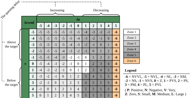
For a system with two inputs and one output like FLOWER, we can list all rules using tabular representation as shown in Fig. 4. Note that in the rule table in Fig. 4, we use linguistic-numeric values to shorten the description of lin-guistic values [15] (e.g., -5 represents NVS; 0 represents Z; 3 represents PM; . . . ).

To better understand the fuzzy controller dynamics, we divide the rule table into six zones as follows:

Zone 1: Rules of this zone maintain the steady-state queu-ing delay around the target. Both e(k) and ∆e(k) remains very close to zero. In consequence, the fuzzy controller must slightly increase or decrease the con-gestion window (denoted ∆cwndin Fig. 4) to rectify

small deviations from the target.

Zone 2: In this zone, e(k) is positive or zero, which means that the queuing delay is respectively either below or equal to the target. In addition, since ∆e(k) is neg-ative or zero, the queuing delay tends to raise and thus moves in the direction of the target. Therefore, based on the increase trend magnitude of the queuing delay, the fuzzy controller must either increase (i.e. ∆cwnd> 0) or decrease (i.e. ∆cwnd< 0) the

conges-tion window to accelerate or decelerate the queuing delay motion to match the target.

Zone 3: In this zone, since e(k) is negative, the queuing delay is above the target. On the other hand, ∆e(k)

is negative or zero, which means that the queuing de-lay tends to increase and hence, in this case, moves away from the target. Consequently, the fuzzy con-troller must decrease the congestion window to com-pensate the increase of the queuing delay.

Zone 4: For this zone, e(k) is negative and ∆e(k) posi-tive, which corresponds to the situation where the queuing delay is above and is decreasing towards the target. As a result, to match the queuing delay to the target, the fuzzy controller needs to accelerate or decelerate the queuing delay motion based on the magnitude of its decrease trend.

Zone 5: Rules of this zone represent the situation where the queuing delay is either below or equal to the tar-get. Moreover, the queuing delay is decreasing away from the target. Thus, e(k) is either positive or zero and ∆e(k) is positive. The fuzzy controller must therefore increase the congestion window to reverse the decrease trend of the queuing delay.

Zone 6 — Congestion Detection Zone: An important feature of FLOWER is its capability to react quickly to congestion events caused by TCP. This feature is integrated in the rule base and can be observed in the last column of the rule table called the conges-tion detecconges-tion zone (see Fig. 4). Concretely, when FLOWER detects a very large decrease in the queu-ing delay (∆e(k) is 5 or PVL), it must immediately reduce to its minimum congestion window (e.g, set to one packet). This case corresponds to the following output: ∆cwnd(k) is -6 or NVVL.

(9)

4.3. Membership functions

A membership function defines the semantic of a lin-guistic value. Let’s A denote a linlin-guistic value and X be a universe of discourse for an input or output of a fuzzy system, i.e, the range of numerical values that the inputs and outputs can take as values. Each linguistic value A is associated with a membership function. This member-ship function quantifies the certainty or membermember-ship de-gree that a numerical value x ∈ X can be classified lin-guistically as A. The set of numerical values of X that a membership function describes as being a linguistic value A is called a fuzzy set.

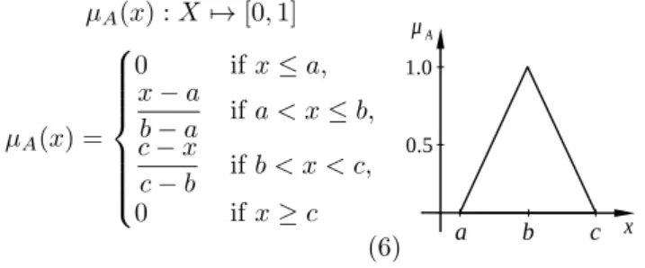
In this paper, we use the most common triangle mem-bership function defined by the three parameters {a, b, c} as follows: µA(x) : X 7→ [0, 1] µA(x) =              0 if x ≤ a, x − a b − a if a < x ≤ b, c − x c − b if b < x < c, 0 if x ≥ c (6)

where a < b < c and b is the center of the triangle mem-bership function (i.e., where it reaches its peak) [15].

Consider, for example, the membership function µP V S

that quantifies the meaning of the linguistic value positive very small for any numerical value x ∈ X:

• if µP V S(x) = 0 then we are certain that x is not

PVS;

• if µP V S(x) = 0.5 then we are only half certain that

x is PVS. It could also be Z with some degree of certainty;

• if µP V S(x) = 1 then we are absolutely certain that

x is PVS.

Fig. 5 shows all the membership functions for the in-puts and the output of the FLOWER fuzzy controller. 4.3.1. Membership functions of e(k)

Since the queue size varies continuously as a function of the network traffic, we need to make the input error e(k) independent of the network state. For this purpose, before introducing e(k) into the fuzzy controller, we express it as follows: e(k) =      e(k) τ × 100 if q(k) ≤ τ, e(k) qmax− τ × 100 if q(k) > τ (7)

where qmax is the maximum queuing delay observed on

the network. Consequently, the membership functions of e(k) is linearly distributed on the universe of discourse [−100, 100] %.

4.3.2. Membership functions of ∆e(k)

The queuing delay is ranging from 0 to the maximum value qmax. Thus, we have

∆e(k) = −(q(k) − q(k − 1)) = −∆q(k) (8) where

q(k) ∈ [0, qmax]

Then, the universe of discourse for ∆e(k) is [−qmax, qmax] ms.

The variation of the queuing delay, and thus ∆e(k), highly depends on the network state. Hence, we need to dynamically adapt the distribution for the membership functions of ∆e(k). In addition, as seen in the rule table in Fig. 6, the congestion detection zone of FLOWER relies only on ∆e(k). Therefore, we must determine a threshold to define this zone. To this end, we use the exponentially weighted moving average (EWMA) of values of ∆e(k). As EWMA has higher weights on recent data than on older data, sudden network condition changes are further taken into account in this average. Consequently, the distribu-tion for the membership funcdistribu-tions of ∆e(k) is as follows:

−qmax, sde−, −3, −2, −1, 0, 1, 2, 3, sde+, qmax

where sde− and sde+ are the EWMA of the negative and

positive values of ∆e(k), respectively. {−qmax, sde−, sde+, qmax}

are respectively initialized with {−5, −4, 4, 5}. These val-ues are updated only when the absolute value of a new value is greater than the absolute value of the initial value. Finally, we underline that, as an effect of the congestion detection zone, when ∆e(k) > sde+, even if the certainty

µP V L(∆e(k)) is small, FLOWER reduces the congestion

window to its initial value.

4.3.3. Membership functions of ∆cwnd(k)

Outside the congestion detection zone, the distribu-tion of ∆cwnd(k) is linear on the universe of discourse [−1, 1] packet. As a consequence, the maximum ramp-up speed of FLOWER is the same as TCP, i.e., one packet per RTT. When operating in the congestion detection zone, ∆cwnd(k) is set to negative infinity to signal FLOWER to reduce to minimum its sending rate. Otherwise, FLOWER will ramp-down at maximum one packet per RTT. 4.4. Fuzzification

Fuzzification is the process of making a numerical value fuzzy so that it can be used by the fuzzy system. When-ever the fuzzification module receives a numerical value x, it converts this value into a corresponding linguistic value by associating a certainty that is quantified by the mem-bership function µA(x).

4.5. Inference mechanism

The inference mechanism derives the fuzzy outputs from the fuzzy inputs obtained by fuzzification, according to the relation defined through fuzzy rules. The main matter is how to interpret the meaning of each rule, i.e., how to

(10)

-1

-2

-3

-4

-5

0

1 2 3

4

5 -1

-2

-3

-4

-5

0 1 2 3 4 5

-1

-2

-3

-4

-5

0 1 2 3 4 5

e(t) (%)

Δe(t) (ms)

Δcwnd(t)

20 sde+

q

_max

sde-

-3

-2

-1

1 2 3

40 60 80 100

-20

-40

-60

-80

-100

.6 .8 1.0

.4

.2

-.2

-.4

-.6

-.8

-1.0

-

∞

-6

-q

_max

Figure 5: The membership functions of the FLOWER fuzzy controller.

determine the influence produced by the premise on the conclusion of the fuzzy rule. To assess this influence, the inference process generally involves in two steps:

1. The certainty of the premise is determined using the fuzzy conjunctive operator (AND);

2. The certainty of the conclusion, influenced by the premise, is determined using the fuzzy implication operator.

To illustrate the general idea of the inference mecha-nism, we consider a simple fuzzy system with two inputs x1 and x2 and one output y. The system is described by

the following rule base of the form:

Ri : If x1 is Ai1 and x2is Ai2Then y is B i_,

for i = 1, 2, . . . , r where Ai

1, Ai2, and Bi are the linguistic values of the

lin-guistic variables x1, x2, and y in the i-th rule Ri. We use

the minimum operator to represent both fuzzy conjunctive and implication operators. Therefore, the certainty of the premise of rule Ri is determined as follows:

µAi(x₀) = µ_(Ai

1AND Ai2)(x1, x2)

= min(µAi

1(x1), µAi2(x2)) (9)

where x0 = (x1, x2). Then, the certainty of rule Ri is

determined as follows:

µRi(y) = min(µAi(x0), µBi(y)) (10)

where µBi(y) is the membership function of the consequent

of rule Ri. The membership function µRi(y) quantifies

how certain rule Ri is when the output y should take on

certain values. In Eq. 10, the minimum operation trun-cates the membership function of the consequent µBi(y)

to produce the membership function µRi(y) (for graphical

representation, see example in Section 4.7). 4.6. Defuzzification

Defuzzification is the process of combining results of the inference mechanism to obtain a numerical output value y. We use the “center-average” defuzzication method which calculates the weighted average of the output mem-bership function centers bi:

y = P ibisupy{µRi(y)} P isupy{µRi(y)} (11)

where sup_y{µRi(y)} is the highest value of µRi(y).

We have finished the description of the three processes fuzzification, inference and defuzzification in a general con-text. For FLOWER, we have x1 = e(k), x2= ∆e(k) and

y = ∆cwnd(k).

4.7. Example of fuzzy controller operations

Consider the example in Fig. 6. Suppose that e(k) = 35 after being converted to the percentage form and ∆e(k) = 1. The fuzzification process using Eq. 6 gives µP V S(e(k)) =

(11)

PS PM Δcwnd(k) .6 .8 .4 .2 Δcwnd = 0.55 PVS e(k) (%) 0 40 PS Δcwnd(k) .6 .4 .2 PVS 0 2 Δe(k) (ms) μ_PVS(Δe(k)) = 1 μ_PVS(e(k)) = 0.25 _min μ μ μ PVS 0 2 PS e(k) (%) 20 60 Δe(k) (ms) PM Δcwnd(k) .6 .8 .4 μ_PVS(Δe(k)) = 1 μPS(e(k)) = 0.75 min μ μ μ

R₁: If e(k) is PVS and Δe(k) is PVS Then Δcwnd(k) is PS

R₂: If e(k) is PS and Δe(k) is PVS Then Δcwnd(k) is PM

μ

Figure 6: Graphical representation of fuzzy controller operations.

Fig. 6 shows the certainties of the membership functions for the inputs and indicates with black vertical lines the numerical values of e(k) and ∆e(k). In this case, by con-sulting the rule table in Fig. 4, we have the following cor-responding rules:

R1: If e(k) is PVS and ∆e(k) is PVS Then ∆cwnd(k) is

PS

R2: If e(k) is PS and ∆e(k) is PVS Then ∆cwnd(k) is

PM

Now, consider the first rule R1. Let x0= (e(k), ∆e(k)),

and thus, using Eq. 9 of the inference mechanism, the cer-tainty of the premise of the rule R1is:

µA1(x0) = min(µP V S(e(k)), µP V S(∆e(k)))

= min(0.25, 1) = 0.25 and then, according to Eq. 10, we have:

µR1(∆cwnd(k)) = min(0.25, µP S(∆cwnd(k)))

The membership function µR1(∆cwnd(k)), which is the

conclusion reached by rule R1, is shown in Fig. 6 as the

blue region of the output membership function µP S(∆cwnd(k))

defining the linguistic value PS. As mentioned in Section 4.5, this blue region is a result from the truncation of the mem-bership function µP S(∆cwnd(k)) by the minimum

opera-tor. As a conclusion for rule R1, we are at most 25%

cer-tain that the ouput ∆cwnd(k) should be a positive small value.

In the same way, for the second rule R2, we have:

µA2(x0) = min(µP S(e(k)), µP V S(∆e(k)))

= min(0.75, 1) = 0.75 and

µR2(∆cwnd(k)) = min(0.75, µP M(∆cwnd(k)))

The membership function µR2(∆cwnd(k)) is shown as the

red region of the output membership function µP M(∆cwnd(k))

defining the linguistic value PM in Fig. 6. Here, we are at most 75% certain that the ouput ∆cwnd(k) should be a positive medium value. Therefore, we are more certain of the conclusion reach by rule R2 than the conclusion reach

by rule R1.

To convert the conclusions of the inference process to a numerical output, we use Eq. 11 of the defuzzification pro-cess. As shown in Fig. 6, the highest values of µR1(∆cwnd(k))

and µR2(∆cwnd(k)) is 0.25 and 0.75, respectively. Thus,

we have:

sup∆cwnd{µR1(∆cwnd(k))} = 0.25

and

(12)

Then, with the output membership function centers b1=

0.4 and b2= 0.6, we have:

∆cwnd(k) = 0.4 × 0.25 + 0.6 × 0.75 0.25 + 0.75 = 0.55

5. Evaluation of FLOWER

We use the network simulator ns-2.35 to validate our new protocol. For this purpose, we have implemented an ns-2 prototype of FLOWER based on LEDBAT module developed by Valenti et al. [16]. The prototype is imple-mented as a Linux congestion control module on top of the TCP-Linux framework [17]. Therefore, simulation re-sults are much closer to a real implementation in the Linux kernel and would allow to easily port our implementation inside the Linux kernel (this also been the case for the LEDBAT module [16]).

We specifically focus on the FLOWER performance in terms of respect to a LBE traffic and latecomer unfairness which are the two major drawbacks of LEDBAT.

5.1. Simulation setup

We use a dumbbell topology where a TCP flow shares a single bottleneck link with a LBE flow (either FLOWER or LEDBAT). Note that to test our protocol, we follow the scenario used in [12] for the sake of comparison. All sources send packets with a size of P = 1500 B. The bottleneck link has a capacity set to C = 10 Mb/s and a one-way prop-agation delay owd ∈ [10, 50, 100, 150, 200, 250] ms. The bottleneck router is a FIFO drop-tail queue with a size of B packets. For convenience, we express the bottleneck buffer B as a ratio to the bandwidth-delay product BDP in terms of packets. Hence, we have B = dn · BDP e = dn · C · 2 · owd/(8 · P )e, where the ratio n ∈ [0.2, 0.4, 06, 0.8, 1.0] and dxe is the ceiling function. Since B must be an integer, we use the ceiling function to get the smallest integer not less than B. We also convert the target τ from millisec-onds to packets as follows: τ (packets) = τ (ms) · C/(8 · P ). In this paper, we use the target queuing delay τ = 100 ms for all simulations. Therefore, τ = 100 ms corresponds to 83.3 packets and is rounded to 84 packets.

5.2. Interaction with TCP

In this section, we study the behavior of FLOWER in the presence of TCP and more specifically, the interac-tion between the FLOWER fuzzy controller and the TCP AIMD (Additive Increase/Multiplicative Decrease) algo-rithm.

5.2.1. Scenario and metrics

Two TCP and LBE flows start at t = 0 s and stop at t = 75 s. In this scenario, owd = 50 ms and B = BDP . To investigate the behavior of one LBE flow in coexistence with one TCP flow, we consider their congestion windows and the queue length of the bottleneck buffer.

5.2.2. Results

Fig. 7 shows both congestion windows (top) as a func-tion of time conjointly with the queue length and the target queuing delay expressed in packets (bottom). The interac-tion between TCP and FLOWER is shown in Fig. 7a. In the slow-start phase, TCP and FLOWER increase expo-nentially their congestion window. Thus, the bottleneck queue fills up quickly until loss. Unlike TCP, FLOWER reduces its congestion window to its initial value which equals to one packet in our implementation. After the slow-start phase, approximatively before t = 3 s, as the bottleneck queue is half-filled but the resulting queuing de-lay is small compared to the target, FLOWER and TCP congestion windows conjointly grow. As the queue still increases because TCP keeps sending packets, FLOWER reduces its sending rate (the target is almost reached) and finally stabilizes its congestion window. After t = 7.5 s, when the queuing delay is close to the target, FLOWER reacts by decreasing its sending rate. Finally, FLOWER reaches the minimum sending rate of one packet per RTT at t = 9.3 s. Slightly afterwards, TCP gets losses and en-ters in its recovery phase. As a consequence, TCP halves its congestion window and the bottleneck queue is drained. TCP re-enters in the congestion avoidance phase at t = 10 s while FLOWER grows at its maximum speed as the queue is not fully filled. FLOWER prevents bottleneck overflow by reducing its sending rate before the knee phase [18] (i.e. when the rate increases gradually but slower than the delay). When TCP halves its congestion window at t = 21.8 s, we observe an abrupt decrease of the queuing delay. Shortly afterwards, FLOWER detects this decrease with the help of the congestion detection scheme, hence it drops to the minimum its congestion window. Therefore, the queue is drained and FLOWER enters in a new cycle. Henceforth, both FLOWER and TCP are in steady state. This first experiment illustrates the good LBE behav-ior of FLOWER in the presence of TCP. Clearly, the fuzzy controller with the congestion detection scheme allows FLOWER to be LBE compliant. In this standard configuration (we recall that B = BDP ), LEDBAT does not behave as a LBE protocol and is too aggressive as shown in Fig. 7b. This figure also illustrates that the LEDBAT P-type con-troller does not react correctly to congestion events. We refer the reader to previous studies [6, 14] for further de-tails on the LEDBAT defective behavior.

In the next section, we extend these measurements to several general networking use-cases in order to exhaus-tively illustrate the good performance of our fuzzy con-troller scheme.

5.3. FLOWER versus LEDBAT performance in coexis-tence with TCP NewReno and TCP Cubic

In this section, we evaluate the impact of FLOWER flows on TCP flows (either NewReno or Cubic) in different network conditions.

(13)

100 200 300 Congestion window (pkts) New Reno FLOWER 0 40 80 120 160 200 0 10 20 30 40 50 60 70 Queue length (pkts) Time (s) Target Queue length

(a) FLOWER vs. TCP NewReno

100 200 300 Congestion window (pkts) New Reno LEDBAT 0 40 80 120 160 200 0 10 20 30 40 50 60 70 Queue length (pkts) Time (s) Target Queue length (b) LEDBAT vs. TCP NewReno Figure 7: TCP and LBE congestion windows and bottleneck queue length as a function of time.

5.3.1. Scenario and metric

We consider x long-lived TCP flows with x LBE flows where x ∈ {2, 5, 10}. The simulation lasts 1200 s where TCP flows start consecutively every 10 s from t = 0 s and keep sending data until the end of simulation. LBE flows start randomly between t = 350 s and t = 450 s in order for TCP to reach the full capacity.

To assess the impact of LBE on TCP, we define the metric rate distribution (X) as the total throughput achieved by all flows Fk where k ∈ {T CP, LBE} over the total

throughput of all flows on the link: Xk=

Fk

FT CP+ FLBE

(12) For each combination of network configuration {owd, B}, we run the simulation 10 times. After each run, we calcu-late the rate distribution over the last 600 seconds. Then, the mean of the 10 metric values is taken as the measured value.

5.3.2. Results

In Fig. 8, using histogram, we group the simulation results into different categories of one-way delay (denoted owd in Fig. 8), and then into subclasses of buffer size given as a ratio to the BDP. For information purpose, note that at the top of the histogram, the equivalent ratio to the BDP is converted as the ratio to the target value given in packets as explained in Section 5.1. This means we express B as the ratio to the target τ in the same way as with the BDP . For instance, looking at Fig. 8, a buffer sized 0.4 of the BDP at owd = 100 ms corresponds to 0.7 of target value in packets. For each buffer size, each stacked column gives the sum of the normalized rates obtained by both TCP and LBE flows. Then, each slice inside a column represents the part obtained by x TCP and x LBE flows given by (12).

Fig. 8a, 8c and 8e show the performance of LEDBAT and FLOWER in the presence of TCP NewReno. We have

selected a set of network configurations following our previ-ous study on the LEDBAT performance issues [6]. These network configurations illustrate a large number of use-cases where LEDBAT performs (in Fig. 8a, 8c and 8e, when the ratio of the bottleneck buffer size to the target τ is largely greater than 1) or does not perform correctly (resp. the reverse). As shown in Fig. 8a, 8c and 8e, LED-BAT obtains sometimes more than TCP NewReno and crosses the fair-share line represented by a dotted line. We then compare the results obtained by FLOWER in these configuration. Fig. 8a, 8c and 8e allow to easily compare the performance of both protocols in identical situation. The results are unequivocal and illustrate that FLOWER behaves as a LBE protocol where LEDBAT fails in realistic cases.

Using the same network configurations as above, we now study the performance of LEDBAT and FLOWER in coexistence with TCP Cubic in Fig. 8b, 8d and 8f. TCP Cubic is more aggressive than TCP NewReno but in those cases, the performance of FLOWER is better than LED-BAT in respect of the LBE principle.

5.4. Intra-protocol fairness

We finally study the interaction between two FLOWER flows to assess their intra-fairness and determine whether FLOWER is not impacted by the latecomer issue. 5.4.1. Scenario and metric

In this scenario, the buffer size B is set to twice the BDP . This configuration is favorable to get the LED-BAT latecomer unfairness phenomenon. The bottleneck link has a one-way delay owd = 50 ms. The first LBE flow starts at t = 0 s and the second starts at t = 20s. Both flows last 150 s. As in 5.2, we draw their congestion windows and the queue length of the bottleneck buffer. 5.4.2. Results

Fig. 9b shows the LEDBAT latecomer issue [16]. The first LEDBAT flow starts when the bottleneck queue is

(14)

0.2 0.4 0.6 0.8

1 0.04 0.07 0.1 0.1 0.2 0.2 0.3 0.5 0.7 0.8 0.3 0.7 1.0 1.3 1.7 0.5 1.0 1.5 2.0 2.5 0.7 1.3 2.0 2.7 3.3 0.8 1.7 2.5 3.3 4.2

Buffer size (ratio to τ in pkts)

TCP

vs. FLO

WER

FLOWER New Reno

0.2 0.4 0.6 0.8 1 0.2 0.4 0.6 0.8 1 0.2 0.4 0.6 0.8 1 0.2 0.4 0.6 0.8 1 0.2 0.4 0.6 0.8 1 0.2 0.4 0.6 0.8 1 0.2 0.4 0.6 0.8 1 Rate distribution

Buffer size (ratio to BDP in pkts)

TCP vs. LED BA T LEDBAT 250 ms 200 ms 150 ms 100 ms 50 ms owd=10 ms

(a) 2 flows TCP NewReno vs. 2 flows LBE

0.2 0.4 0.6 0.8

1 0.04 0.07 0.1 0.1 0.2 0.2 0.3 0.5 0.7 0.8 0.3 0.7 1.0 1.3 1.7 0.5 1.0 1.5 2.0 2.5 0.7 1.3 2.0 2.7 3.3 0.8 1.7 2.5 3.3 4.2

TCP

vs. FLO

WER

FLOWER New Reno

(b) 2 flows TCP Cubic vs. 2 flows LBE

0.2 0.4 0.6 0.8

1 0.04 0.07 0.1 0.1 0.2 0.2 0.3 0.5 0.7 0.8 0.3 0.7 1.0 1.3 1.7 0.5 1.0 1.5 2.0 2.5 0.7 1.3 2.0 2.7 3.3 0.8 1.7 2.5 3.3 4.2

TCP

vs. FLO

WER

FLOWER New Reno

(c) 5 flows TCP NewReno vs. 5 flows LBE

0.2 0.4 0.6 0.8

1 0.04 0.07 0.1 0.1 0.2 0.2 0.3 0.5 0.7 0.8 0.3 0.7 1.0 1.3 1.7 0.5 1.0 1.5 2.0 2.5 0.7 1.3 2.0 2.7 3.3 0.8 1.7 2.5 3.3 4.2

TCP vs. FLO WER FLOWER Cubic 0.2 0.4 0.6 0.8 1 0.2 0.4 0.6 0.8 1 0.2 0.4 0.6 0.8 1 0.2 0.4 0.6 0.8 1 0.2 0.4 0.6 0.8 1 0.2 0.4 0.6 0.8 1 0.2 0.4 0.6 0.8 1 Rate distribution

(d) 5 flows TCP Cubic vs. 5 flows LBE

0.2 0.4 0.6 0.8

1 0.04 0.07 0.1 0.1 0.2 0.2 0.3 0.5 0.7 0.8 0.3 0.7 1.0 1.3 1.7 0.5 1.0 1.5 2.0 2.5 0.7 1.3 2.0 2.7 3.3 0.8 1.7 2.5 3.3 4.2

TCP

vs. FLO

WER

FLOWER New Reno

(e) 10 flows TCP NewReno vs. 10 flows LBE

0.2 0.4 0.6 0.8

1 0.04 0.07 0.1 0.1 0.2 0.2 0.3 0.5 0.7 0.8 0.3 0.7 1.0 1.3 1.7 0.5 1.0 1.5 2.0 2.5 0.7 1.3 2.0 2.7 3.3 0.8 1.7 2.5 3.3 4.2

TCP

vs. FLO

WER

FLOWER New Reno

(f) 10 flows TCP Cubic vs. 10 flows LBE Figure 8: Rate distribution of TCP and LBE flows.

empty, and as a result, senses a base delay. When the sec-ond LEDBAT flow starts at t = 20 s, the queue is filled with ≈ 50 packets. Consequently, the second flow esti-mates a higher base delay including the queuing delay of the first one. Since its estimated queuing delays are below the target delay, the second flow raises its sending rate. As a result, the first one senses an increasing queuing delay

and begins to decelerate. Finally, it reaches its minimum rate at t = 131 s as shown in Fig. 9b. On the contrary, FLOWER does not inherit this latecomer issue thanks to the congestion detection scheme described in Section 4 as shown in Fig. 9a. This experiment demonstrates that two FLOWER flows can now share fairly the link capacity.

(15)

100 200 300 400 500 Congestion window (pkts) FLOWER 1 FLOWER 2 0 40 80 120 160 200 0 20 40 60 80 100 120 140 Queue length (pkts) Time (s) Target Queue length (a) FLOWER 0 100 200 300 Congestion window (pkts) LEDBAT 1 LEDBAT 2 0 40 80 120 160 200 0 20 40 60 80 100 120 140 Queue length (pkts) Time (s) Target Queue length (b) LEDBAT Figure 9: LBE congestion windows and bottleneck queue length as a function of time.

the goal of slow-start is to create a spike in queuing delay when a new FLOWER flow enters in the network. This queuing delay spike should be detected by other ongoing FLOWER flows with the help of the congestion detection zone in the rule table of the fuzzy controller. However, when the bottleneck buffer size is not large enough or when the bottleneck is heavily congested, this queuing de-lay spike (caused by the slow-start) might be too small to be detected by FLOWER. In general and in this context (i.e. bottleneck heavily congested or small buffer size), the performance of delay-based congestion control proto-cols heavily suffer from the inaccuracy of the estimated delay as discussed [3].

6. Coexistence of FLOWER and AQM

Active Queue Management (AQM) has been an active research field starting from the QoS epoch. While many schemes have been proposed, their deployment seems very limited although many of them are available in the GNU/Linux kernel. However, recent concern about the excessive net-work end-to-end delay makes AQM an up to date and hot topic at the IETF today. AQM is usually considered as the best solution to solve this bufferbloat problem [19, 20]. Unfortunately, LBE transport protocols are designed to work mainly under a DropTail queuing discipline.

In the presence of AQM, LEDBAT loses its LBE char-acteristic and behaves like standard TCP as shown by the authors of [21] and of [22, 12]. LEDBAT RFC also admits this fact [4]: “If Active Queue Management is configured to drop or ECN-mark packets before the LEDBAT flow starts reacting to persistent queue buildup, LEDBAT re-verts to standard TCP behavior rather than yielding to other TCP flows”. Therefore, when designing a new LBE protocol (or any kind of novel transport protocol), it is important to study its coexistence with AQM schemes.

In this section, we evaluate the impact of AQM such as RED [23], CoDel [24] and PIE [25] on the LBE-compliance of FLOWER in the presence of standard TCP connections.

We chose to limit our study to these three AQMs as they currently compete at the IETF as a potential solution for the bufferbloat problem [20, 19]. To ease the comparison, we directly employ the scripts used by the authors of this excellent study [12], which are available at [26].

6.1. Active Queue Management Schemes

Before diving into the results, we briefly review and recall the principle behind each AQM tested.

6.1.1. Random Early Detection (RED)

RED randomly dropped packets with a probability p, calculated based on the Exponential Weighted Moving Av-erage (EWMA) qavgof the instantaneous queue length as

follows: p(qavg) =        0 0 ≤ qavg≤ minth, qavg− minth maxth− minth

pmax minth< qavg≤ maxth,

1 qavg> maxth

(13) where

minth: the minimum threshold,

maxth: the maximum threshold,

pmax: the maximum probability for packet dropping at

the maximum threshold.

In this study, we use the default version of RED in ns-2. In this version, the gentle mode is enabled to make RED more robust; the minth and maxth are

automati-cally configured as a function of the target average delay targetdelay , which has a default value of 5 ms.

6.1.2. Controlled Delay (CoDel)

The goal of CoDel is to keep the minimum queuing delay (or sojourn delay) experienced by packets in a fixed interval (100 ms by default) below a target delay (5 ms by default). Therefore, CoDel starts to drop selected packets

(16)

when the minimum queuing delay is higher than the target delay. Each time CoDel drops a packet, it sets the next dropping time based on the number of drops since the beginning of the dropping state, as follows:

nextDropT ime = lastDropT ime +√ interval numOf Drops

(14) For our test, we use the ns-2 CoDel implementation provided by the scripts of [12].

6.1.3. Proportional Integral Controller Enhanced (PIE) Similar to CoDel, PIE keeps the queuing delay around a target delay, which has a default value of 20 ms. How-ever, instead of monitoring the real delay for each packet like CoDel, PIE estimates the current queuing delay based on the queue draining rate using Little’s law. To determine the dropping probability every tupdatetime units, PIE

em-ploys a PI-type controller that takes into account both the current queuing delay and its trend:

p = p + α · (queuingDelay − targetDelay)

+ β · (queuingDelay − lastQueuingDelay) (15) where the factors α and β are respectively set to 0.125 and 1.25 by default. The ns-2 implementation of PIE used can be found at [27].

6.2. Scenario and Metrics

We consider five long-lived standard TCP flows con-jointly with five LBE flows. All flows start at time t = 0. In this scenario, owd = 50 ms and B = 250 pkts = 3 × BDP to reproduce the bufferbloat.

To evaluate the interaction between LBE protocols (LED-BAT, FLOWER) and AQM schemes (RED, CoDel, PIE), we measure the rate distribution of TCP XT CP, the

aver-age queue length E[Q] in terms of packet, and the bufferbloat intensity defined as E[Q]/B. Note that in [12], the authors denote XT CP as T CP %.

For each combination of LBE protocols and AQM schemes, we run the simulation ten times and each run lasts for 60 s. The mean of the metric values is then taken as the mea-sured values.

6.3. Impact of AQM Schemes on LBE Protocols

We present the simulation results in Figure 10 using a parallel coordinate plot. The left and right y-axes cor-respond to the bufferbloat intensity E[Q]/B and the rate distribution of TCP, respectively. In the parallel coordi-nate plot, a line connecting these two metrics represents the interaction of each combination of AQM schemes and LBE protocols. The ideal interaction is illustrated by the green oblique region in Figure 10, in which the queuing delay is low while the LBE traffic remains low-priority.

Under DropTail (denoted DT in Fig. 10), TCP con-tinuously fills up the buffer until loss and therefore maxi-mizes the bufferbloat intensity, as shown in Figure 10. As

Figure 10: Impact of AQM on LBE protocols.

for LEDBAT and FLOWER, in this case, they are both LBE-compliant, which are represented by TCP shares ap-proaching one. We recall that the goal of LEDBAT and FLOWER is to keep the queuing delay around a fixed tar-get. Nevertheless, this choice of design only limits the exacerbation of bufferbloat but does not solve it.

Figure 10 clearly shows that employing an AQM scheme solves the bufferbloat issue. However, such an AQM scheme also compromises the low-priority characteristic of LBE protocols and raises their aggressiveness towards TCP. In this case, LEDBAT competes quite fairly with TCP. The results for LEDBAT are actually in accordance with the study in [12]. Regarding the new protocol, in all cases, FLOWER is always more LBE-compliant than LEDBAT and tends towards the ideal region. There are two reasons behind this outcome. First, FLOWER has a congestion detection zone in its fuzzy rule base that allows it to re-act better than LEDBAT in front of congestion. Second, FLOWER resets its congestion window to minimum in case of loss to alleviate its impact on higher priority flows. Both allows to make FLOWER compliant to perform with AQM schemes.

7. Conclusion

We propose FLOWER, a new delay-based congestion control protocol designed to provide a LBE service us-ing results from the fuzzy logic area. The main goal of FLOWER is to overcome both major LEDBAT drawbacks: aggressiveness and latecomer unfairness, while being LBE compliant. Our simulation study over a wide range of network use-cases shows that FLOWER performs better than LEDBAT in case where it usually fails. To the best of our knowledge, FLOWER is the first solution that solves both the aggressiveness issue inherent to LEDBAT pro-tocol and the fairness issue. Last but not least, we fi-nally showed that FLOWER remains compliant with AQM schemes that aim to mitigate the bufferbloat issue.

(17)

Acknowlegdements

The authors wish to thank CNES and Thales Alenia Space for funding and C´edric Baudoin, Emmanuel Dubois, Patrick G´elard for numerous discussions on this study.

References

[1] S. Blake, D. Black, M. Carlson, E. Davies, Z. Wang, W. Weiss, An Architecture for Differentiated Services, RFC 2475 (Dec. 1998).

[2] V. Cerf, V. Jacobson, N. Weaver, J. Gettys, BufferBloat: What’s Wrong with the Internet?, Queue, ACM 9 (12) (2011) 10–20.

[3] D. Ros, M. Welzl, Less-than-Best-Effort Service: A Survey of End-to-End Approaches, Commun. Surveys Tutorials, IEEE 15 (2) (2013) 898–908.

[4] S. Shalunov, G. Hazel, J. Iyengar, M. Kuehlewind, Low Ex-tra Delay Background Transport (LEDBAT), RFC 6817 (Dec. 2012).

[5] G. Carofiglio, L. Muscariello, D. Rossi, C. Testa, A hands-on Assessment of Transport Protocols with Lower than Best Effort Priority, in: IEEE LCN, 2010.

[6] S. Q. V. Trang, N. Kuhn, E. Lochin, C. Baudoin, E. Dubois, P. Gelard, On the existence of optimal LEDBAT parameters, in: IEEE ICC, 2014.

[7] N. Kuhn, O. Mehani, A. Sathiaseelan, E. Lochin, Less-than-Best-Effort Capacity Sharing over High BDP Networks with LEDBAT, in: IEEE VTC Fall, 2013.

[8] D. Ros, M. Welzl, Assessing LEDBAT’s Delay Impact, Com-mun. Lett., IEEE 17 (5) (2013) 1044–1047.

[9] G. Carofiglio, L. Muscariello, D. Rossi, C. Testa, S. Valenti, Rethinking the Low Extra Delay Background Transport (LED-BAT) Protocol, Comput. Netw. 57 (8) (2013) 1838–1852. [10] A. Venkataramani, R. Kokku, M. Dahlin, TCP Nice: a

mecha-nism for background transfers, SIGOPS Oper. Syst. Rev. 36 (SI) (2002) 329–343.

[11] A. Kuzmanovic, E. W. Knightly, TCP-LP: low-priority ser-vice via end-point congestion control, IEEE/ACM Trans. Netw. 14 (4) (2006) 739–752.

[12] Y. Gong, D. Rossi, C. Testa, S. Valenti, M. T¨aht, Fighting the bufferbloat: on the coexistence of AQM and low priority congestion control, Comput. Netw. 65 (2014) 255–267. [13] A. Abu, S. Gordon, A Dynamic Algorithm for Stabilising

LED-BAT Congestion Window, in: ICCNT, 2010.

[14] D. R. Giovanna Carofiglio, Luca Muscariello, S. Valenti, The Quest for LEDBAT Fairness, in: IEEE GLOBECOM, 2010. [15] K. Passino, S. Yurkovich, Fuzzy Control, Addison-Wesley, 1998. [16] D. Rossi, C. Testa, S. Valenti, L. Muscariello, LEDBAT: The New BitTorrent Congestion Control Protocol, in: ICCCN, 2010. [17] D. X. Wei, P. Cao, NS-2 TCP-Linux: An NS-2 TCP Imple-mentation with Congestion Control Algorithms from Linux, in: Proc. Workshop Ns-2: The IP Network Simulator, 2006. [18] D.-M. Chiu, R. Jain, Analysis of the Increase and Decrease

Algorithms for Congestion Avoidance in Computer Networks, Comput. Netw. ISDN Syst. 17 (1) (1989) 1–14.

[19] N. Khademi, D. Ros, M. Welzl, The new aqm kids on the block: An experimental evaluation of codel and pie, in: IEEE Con-ference on Computer Communications Workshops (INFOCOM WKSHPS), 2014, pp. 85–90.

[20] N. Kuhn, E. Lochin, O. Mehani, Revisiting old friends: Is codel really achieving what red cannot?, in: Proceedings of the 2014 ACM SIGCOMM Workshop on Capacity Sharing Work-shop, CSWS ’14, ACM, New York, NY, USA, 2014, pp. 3–8. doi:10.1145/2630088.2630094.

URL http://doi.acm.org/10.1145/2630088.2630094

[21] J. Schneider, J. Wagner, R. Winter, H. Kolbe, Out of my way -evaluating Low Extra Delay Background Transport in an ADSL access network, in: Teletraffic Congress (ITC), 2010 22nd In-ternational, 2010, pp. 1–8.

[22] Y. Gong, D. Rossi, E. Leonardi, Modeling the interdependency of low-priority congestion control and active queue manage-ment, in: 2013 25th International Teletraffic Congress (ITC), 2013, pp. 1–9.

[23] S. Floyd, V. Jacobson, Random early detection gateways for congestion avoidance, IEEE/ACM Transactions on Networking 1 (4) (1993) 397–413. doi:10.1109/90.251892.

[24] K. Nichols, V. Jacobson, Controlling queue delay, Communica-tions of the ACM 55 (7) (2012) 42–50.

[25] R. Pan, P. Natarajan, C. Piglione, M. Prabhu, V. Subramanian, F. Baker, B. VerSteeg, PIE: A lightweight control scheme to ad-dress the bufferbloat problem, in: IEEE 14th International Con-ference on High Performance Switching and Routing (HPSR), 2013, pp. 148–155.

[26] http://perso.telecom-paristech.fr/ drossi/index.php?n=Dataset.LEDBATAQM. [27] https://heim.ifi.uio.no/ naeemk/research/PIE/ns-2/.