HAL Id: hal-03197457
https://hal.archives-ouvertes.fr/hal-03197457
Submitted on 13 Apr 2021
HAL is a multi-disciplinary open access
archive for the deposit and dissemination of
sci-entific research documents, whether they are
pub-lished or not. The documents may come from
teaching and research institutions in France or
abroad, or from public or private research centers.
L’archive ouverte pluridisciplinaire HAL, est
destinée au dépôt et à la diffusion de documents
scientifiques de niveau recherche, publiés ou non,
émanant des établissements d’enseignement et de
recherche français ou étrangers, des laboratoires
publics ou privés.
Faster Muscle Segmentation and Propagation in
Volumetric Ultrasound
Dawood Al Chanti, Vanessa Gonzalez Duque, Marion Crouzier, Antoine
Nordez, Lilian Lacourpaille, Diana Mateus
To cite this version:
Dawood Al Chanti, Vanessa Gonzalez Duque, Marion Crouzier, Antoine Nordez, Lilian Lacourpaille,
et al.. IFSS-Net: Interactive Few-Shot Siamese Network for Faster Muscle Segmentation and
Propa-gation in Volumetric Ultrasound. IEEE Transactions on Medical Imaging, Institute of Electrical and
Electronics Engineers, 2021, pp.1-14. �10.1109/TMI.2021.3058303�. �hal-03197457�
IEEE TRANSACTIONS ON MEDICAL IMAGING, VOL. XX, NO. XX, XXXX 2020 1
IFSS-Net: Interactive Few-Shot Siamese
Network for Faster Muscles Segmentation and
Propagation in 3-D Freehand Ultrasound
Dawood Al Chanti, Vanessa Gonzalez Duque, Marion Crouzier, Antoine Nordez, Lilian Lacourpaille, and
Diana Mateus
Abstract—We present an accurate, fast and efficient method for segmentation and muscle mask propagation in 3D freehand ultrasound data, towards accurate volume quantification. To this end, we propose a deep Siamese 3D Encoder-Decoder network that captures the evolution of the muscle appearance and shape for contiguous slices and uses it to propagate a reference mask annotated by a clinical expert. To handle longer changes of the muscle shape over the entire volume and to provide an accurate propagation, we devised a Bidirectional Long Short Term Memory module. To train our model with a minimal amount of training samples, we propose a strategy to combine learning from few annotated 2D ultrasound slices with se-quential pseudo-labeling of the unannotated slices. To pro-mote few-shot learning, we propose a decremental update of the objective function to guide the model convergence in the absence of large amounts of annotated data. Finally, to handle the class-imbalance between foreground and back-ground muscle pixels, we propose a parametric Tversky loss function that learns to adaptively penalize false pos-itives and false negatives. We validate our approach for the segmentation, label propagation, and volume computation of the three low-limb muscles on a dataset of 44 subjects. We achieve a dice score coefficient of over 95 % and a small fraction of error with 1.6035 ± 0.587.
Index Terms—3D Ultrasound, Few-Shot annotation, Mask propagation, Pseudo labelling, Segmentation.
I. INTRODUCTION
Q
UANTIFICATION of muscle volume is a useful biomarker for disease degenerative neuromuscular dis-ease progression or sport performance [1]. Measuring muscle volume often requires the segmentation of 3D images. While Magnetic Resonance (MR) is the modality of preference for imaging muscles, 3D Ultrasound (US) offers a real-time, inexpensive, and portable alternative. The motivation of our work is to assist the segmentation and volume computation of the low limb muscles from 3D freehand ultrasound images.This work has been supported in part by the European Regional Development. Fund, the Pays de la Loire region on the Connect Talent scheme (MILCOM Project) and Nantes M ´etropole.
Dawood Al Chanti, Vanessa Gonzalez Duque and Diana Mateus are with ´Ecole Centrale de Nantes, Laboratoire des Sciences du Num ´erique de Nantes LS2N, UMR CNRS 6004 Nantes, France (e-mail:dawood.alchanti@ls2n.fr).
Marion Crouzier, Antoine Nordez, and Lilian Lacourpaille are with Uni-versit ´e de Nantes, Laboratoire “Movement - Interactions - Performance”, MIP, EA 4334, F-44000 Nantes, France.
However, the methods here developed are general and may be of interest for other clinical applications requiring the segmentation of organs in 3D ultrasound images [2], [3], [24]. In spite of being very time consuming and operator de-pendent, some studies still rely on fully manual segmentation of 3D anatomical structures [4]–[7]. It is therefore essential to develop automatic segmentation methods to assist such studies. In the case of muscle segmentation in US images, an automatic method should be able to address several challenges including the anatomical variability, the lack of contrast or texture differences between individual muscles, as well as the quality of the acquired data [8].
Deep learning-based methods have made successful progress in the analysis of ultrasound images and videos for fetal localization [9], breast and liver lesions classification [10], [11], and cervical muscle segmentation [12]. The success of such fully-supervised methods relies on the availability of large annotated datasets requiring the annotation by clinical experts at scale. Annotating large amounts of ultrasound images is a non-trivial, expensive, and time-consuming task, especially when dealing with 3D or sequential data.
The interest has recently shifted towards learning from a limited quantity of annotated data, using, for instance, few-shot learning [13] or self-supervision [14]. To learn representations from unlabelled input data, self-learning methods commonly rely on auxiliary tasks, such as image reconstruction [15], [16] or context restoration [17]. Self-supervision may also exploit pseudo-labelling [18] wherein unannotated data are relabelled and reused to fine-tune the trained model. In this paper, we propose a novel deep learning segmentation method for 3-D or sequential US data, which requires a reduced amount of expert annotated slices (few-shot) and leverages unannotated slices through sequential pseudo-labelling.
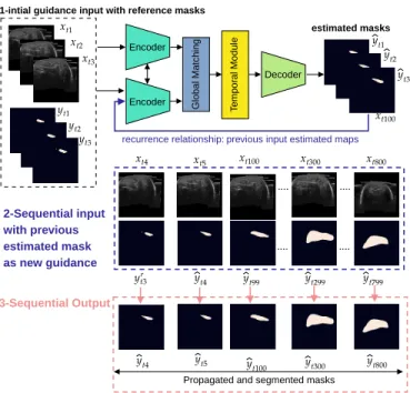
To produce a fast and accurate muscle segmentation, suit-able for relisuit-able volume computation, we design a minimal interactive setting. Explicitly, we ask the expert to provide as initialization the first three muscle’s masks. Similar to Wug et.al. [19], we leverage the spatio-temporal coherence over the slices of a sequence or volume, to propagate the reference masks. In practice, we deploy a Siamese network to capture the representation of contiguous slices, while handling longer changes of the muscle shape done with a Bidirectional Long Short Term Memory (Bi-CLSTM). An overview of our
proposed method, “IFSS-Net,” can be seen in Fig. 1. Encoder Encoder Decoder G lo b a l M a tc h in g T e m p o ra l M o d u le
recurrence relationship: previous input estimated maps 1-intial guidance input with reference masks
estimated masks
Propagated and segmented masks
3-Sequential Output 2-Sequential input with previous estimated mask as new guidance
Fig. 1. Mask Propagation with end-to-end IFSS-Net. Shown here is
an example propagation of foreground mask from the first three slices to the rest of volume slices. The model provides a recurrence feedback loop for self-guidance purposes and to replace the user interaction while keeping it minimal.
To guarantee the model convergence with limited annotated data, we propose a decremental learning strategy. While we start feeding volumes with labeled slices, we progressively reduce the proportion of expert annotations replacing missing annotations with predictions from the model. Finally, to han-dle the class-imbalance between foreground and background pixels, we modify the Tversky loss [37] to adaptively learn the weights that penalize false positive and false negative cases.
We validate our approach for the segmentation, label propa-gation, and volume computation of the three low-limb muscles, namely, the Gastrocnemius Medialis (GM), the Lateralis (GL), and the Soleus (SOL). We consider a dataset of 44 subjects and 61600 ± 5000 images, split into 29 participants (40600 ± 3295 images) for training, and 5 participants (7000±568 images) for validation. Only 3.5 % (1420 ± 136 images) of the annotated training set were required to train our model while the rest of the unannotated images were exploited through sequential pseudo-labeling. The model’s generalization was evaluated over a test set of 10 participants, resulting in a dice score coefficient of over 95 %. We train our “IFSS-Net” network under the weak (3.5 % annotated data) and fully supervised (100 % annotated data) settings, and compared the results to a “3D U-Net” baseline trained in a fully supervised manner. We also compare our model with a state of the art Siamese propagation network within an interactive setting [19]. The main contributions of our work are:
1) A novel deep learning method for segmentation and muscle mask propagation in 3D freehand US data, towards accurate volume quantification.
2) A strategy to combine learning from few annotated
2D US slices with sequential pseudo-labeling of the unannotated slices.
3) A bidirectional spatiotemporal model to adapt to com-plex muscle shape and structure over a longer range. 4) A decremental update of the objective function to guide
the model convergence in the absence of large amounts of annotated data and to induce a few-shot setting. 5) Proposing a parametric Tversky loss function that learns
to adaptively penalize false positives and false negatives.
II. RELATEDWORK
Visual Object Tracking is similar to our mask propagation problem: given a target specified on the first frame, the goal is to follow its evolution on the following frames. In Computer Vision, Siamese networks are a common tracking tool as they are capable of learning similarities to identify related regions in contiguous frames [19]–[23]. When confronted with videos, these methods track either a bounding box around the object [20], [21] or a reference segmentation mask [19]. Recently, Siamese networks have been applied to medical images, for landmark tracking in liver ultrasound sequences [24], or similar to us, for tracking organs from one slice to the next in volumetric US data [2]. Dunnhofer et.al. [2] used a Siamese network for knee cartilage tracking in ultrasound images. The model accepts as input a target image and search area cropped using a manual bounding box. Restricting the search area eases the segmentation task. Our problem differs in that we segment and propagate masks over the slices of a full volume while avoiding to rely on costly manual priors such as bounding boxes.
Our work builds upon the fully-convolutional Siamese architecture “PG-Net” proposed by Wug et.al. [19], which considers both the detection and propagation of a target object in motion. While “PG-Net” produces sharp masks, it leads to unsmooth temporal transitions, which limits its performance when applied to sequential ultrasound data. PG-Net considers only the spatial information within a 2D image before propagating over time with a Recurrent Neural Network (RNN). To enforce mask smoothness, we design a recurrence relationship that connects predictions over time, similar to Hu et.al. [25] and Perazzi et.al. [26]. Such recurrence enables refining previous 2D masks when making new mask predicting predictions. Also, similar to Khoreva et.al. [27], who consider future pixels, we model the muscle pixels in the past and future slices by integrating a Bidirectional Convolutional Long-Short-Term Memory (Bi-CLSTM) [28] model. With the recurrence relationships and the Bi-CLSTM module, we effectively en-force temporal smoothness while taking full advantage of the structural changes along the volume.
To reinforce the learning of local spatio-temporal patterns (instead of only spatial as in [19]), we introduce Atrous Separable Convolutions (ASC) [29] in our model. 3D ASC differs from the typical 3D convolutional operator by an adaptable dilation rate that adjusts the filter’s field-of-view. Thereby, 3D ASC capture contextual information at multiple scales. However, ASC may also produce less sharp masks at the boundaries. Prior work has handled this issue with
AUTHOR et al.: PREPARATION OF PAPERS FOR IEEE TRANSACTIONS ON MEDICAL IMAGING 3
auxiliary refinement [30] or reconstruction [16] tasks. Herein, we rely on a series of 3D ASC (applied to the xyz planes) connected in a recurrently fashion to interpret the full context, while propagating contextual information in the bidirectional z-direction with the Bi-CLSTM.
Pseudo Labelling is a semi-supervised strategy to cope with the difficulty of collecting annotations for large datasets. The strategy [31] consists in using the predictions of a deep network as pseudo-labels to retrain the network with addi-tionally unlabeled data points. More recently, pseudo-labeling has been applied to classification and segmentation problems [18], [32], [33], as well as for correcting noisy labels in the context of active learning [35]. In this paper, we focus on training a segmentation model at the lowest annotation cost while leveraging pseudo-labeling on the high amount of unannotated slices to refine our propagation model. Unlike prior work, we do not split learning into the two classical separated stages: training over labeled data and re-tuning over pseudo labels. Instead, we design a pseudo-labeling scheme for sequential data, taking advantage of the spatiotemporal smoothness between slices. We start from an annotated image and as we move through the sequence and reach an unlabeled slice, we adapt the objective function to compare the current mask prediction with its previous slice pseudo-label.
Handling Unbalanced Data. Using a Dice loss is un-favorable to small structures as a few misclassified pixels may lead to large score drops. To better detect small le-sions, Salehi et.al. [37] introduced the Tversky loss, which generalizes the Dice and Fβ scores, and achieves a
trade-off between precision and recall. Typically, the Tversky index hyper-parameters α and β controlling the penalties for false positives and false negatives are set manually [37]. In this paper, we address class imbalance during training and propose a parametric loss function based on the Tversky index where α and β are learned.
III. METHOD
Consider a volumetric US image is a stack of 2D slices along the z−direction. Given such dataset, we ask a clinical expert to provide the annotation of three such 2D slices for the target muscle (SOL, GL or GM). The objective of this work is then to automatically segment the remainder of the volume by relying on additional poor/partial annotations. Since modeling the segmentation of the full 3D volume at once is intractable, we formulate the segmentation as the propagation of the provided annotations. We model the problem in a spatio-temporal fashion, where the spatio-temporal dimension is associated with the depth of the volume. We process the data with a sliding window treating a partial sub-volume at time.
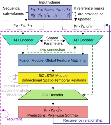
Observing that semantic features learned in an image seg-mentation task and appearance features learned in a similarity matching task complement each other, we combine 3D U-Net for feature extraction and segmentation with a Siamese tracking framework for muscle propagation. A general block diagram is demonstrated in Fig. 2. Our IFSS-Net architecture is composed of two twin 3D encoders with shared parameters. The first captures feature representations from US sub-volumes
Input volume Shared 3-D Encoder Sequential sub-volumes 3-D Encoder If reference masks
Fusion Module: Global Feature Matching
BiCLSTM Module
Bidirectional Spatio-Temporal Relations
3-D Decoder
Predictions: Pixel-wise Softmax
Recurrence relationship
W
shared weights across the whole
sequence Parameters are provided or updated recurrent skip connection
Fig. 2. Our network architecture. The network consists of two twins
encoders, a fusion module, a temporal module, and a decoder.
while the second captures representations from the segmenta-tion masks. The fusion module for global feature matching fuses and matches the current muscle feature representation with the previous time step mask representation. A memory module via Bi-CLSTM captures the spatial and depth changes from the previous, current and future slices. A 3D decoder maps the spatio-temporal information into a pixel-wise pre-diction. A recurrence feedback loop from the output to the mask encoding stream replaces the user interaction to keep it minimal. The whole model M is trained in a recurrent fashion using Truncated Back-propagation Through Time (TBPTT) [38]. Our objective function based on the parametric Tversky index is updated using labeled and pseudo-labeled data in a decremental fashion over upcoming subjects of the training dataset. The process ensures that the model has firstly learned proper and relevant target muscle features from the annotated set, before adding noisy pseudo-labeled slices.
IFSS-Net firstly receives as an input a reference US sub-volume images with its annotated sub-sub-volume masks. This step helps the IFSS-Net to discover the voxels locations of the target muscle to be localized, by matching the spatial appear-ance features (muscle textures and patterns learned from spa-tial 2D slice) and depth deformation features (complex muscle deformation within the changing depth direction, we refer to as temporal information) at the reference US sub-volume. Then, IFSS-Net receives sequentially the subsequent target muscle sub-volume with their previous sub-volume masks estimations. This recurrence relationship promotes the propagation of the previous sub-volume mask estimation to the current target muscle. A cooperating Bi-CLSTM module allows capturing
both the appearance and the depth deformations within the changing depth direction, which we refer to as spatiotemporal features. Moreover, the Bi-CLSTM keeps relevant information from the past and future encoded spatiotemporal features through the gating mechanism. Thereby, Bi-CLSTM is suit-able for refining the mask propagation process using global contexts, i.e. the entire volume. In this way, the proposed IFSS-Net automatically segments the target in every subsequent US sub-volume.
A. Problem Formulation
The dataset used for this work is composed of 3D ultrasound images of low limb muscles V and their respective annotated masks Y for SOL, GL and GM. We denote this data as D = {Vi, Yi}ni=1, where n indicating the number of patients. Each
pair (Vi, Yi) represents an ordered sequence of T stacked
2D gray-scale US slice and their stacked annotated binary masks Yi = {ysoli , y
gl i , y
gm
i } indicating the localization of
the muscles. The depth of the volume is denoted as T ∈ N, being variable among different patients and muscles. Hence,Vi
can be expressed as {x1, ..., xt, ...xT} ∈ RT ×512×512×1
and yi for a certain muscle (e.g. ysoli ) can be expressed
as {y1, ..., yt, ...yT} ∈ {0, 1}T ×512×512×2, with 2 channels
representing the foreground and the background.
The input: formally, we sample from a full volume Vi a
set of sub-volumes vi through rolling a sliding window of
size w with step size of 1. Thereby, out of T 2D slices, we create a new set of T − w + 1 overlapped sub-volumes Vini , where Vini = {vi,1, vi,2, ..., vi,t=k, ..., vi,T −w+1}. At
a given time step t = k, with time step representing the index of a sub-volume corresponding to its depth in the z-stack, a sub-volume vi,k is then composed of w 2D US slices
{xi,k, xi,k+1, xi,k+2, .., xi,k+w}. The corresponding previous
estimated sub-volume masks at time step t = k − 1 is ˆyi,k−1,
composed of {ˆyi,k−1, ˆyi,k, ˆyi,k+1, ..., ˆyi,k+w−1}. Therefore,
Vini = {vi,1, ..., vi,4, ..., vi,t=k, ..., vi,T −w+1} and ˆY in
i =
{yi,1, ..., ˆyi,3, ..., ˆyi,t=k−1, ..., ˆyi,T −w} are fed sequentially to
the network. Fig. 3 demonstrates an input example of sub-volumes composed of 3-stacked images (w = 3) with overlap.
with
Reference sequential sub-volumes with previous estimations
Fig. 3. Sequential input of sub-volume with their corresponding
previ-ous time step estimated masks. We can think about it as 3D+time.
The model: we can think of our model M as
simultane-ously learning local spatio-temporal features from 3D data for segmenting muscles, and global spatio-temporal features for propagating estimated masks through time.
The output: for each sub-volume vi in a set
Vin, the estimated sub-volume masks Yˆin =
{yi,t=1, ˆyi,t=2, ..., ˆyi,t=k, ..., ˆyi,t=T −w} are generated
and fed back to the input. During the training stage, the set of sub-volume estimations ˆYin are considered to update the loss function. During inference, only the first three annotated masks are provided by the expert. For clarity, we will drop the patient index i in the rest of the paper.
B. Network Structure
1) Siamese 3D Encoders: The first 3D Encoder (Eφ(θ))
processes the sub-volumes Vinsequentially by taking at each time step t a sub-volume vt∈ Rw×512×512×1 and modeling
its local appearance and depth deformation simultaneously. Typically, 3D convolutional operators are more appropriate for learning to extract spatio-temporal features compared to 2D convolutional operators. In this study, we mainly use 3D Atrous Separable Convolutions (3D ASC).
Each of the encoders Eφ(θ) and Eϕ(θ) has the same
configuration and shared weights θ. During the training phase, weight updates are mirrored across both sub-networks. We extract the local spatio-temporal features encoded from the US sub-volume vt at certain time step (depth) t by Eφ(θ).
Then, those spatio-temporal features are aggregated to Eϕ(θ)
using skip connections [40]. This aggregation process helps Eϕ(θ) to update the encoders weights θ to a better state as
it has already accessed the previous location of the estimated muscle yt−1.
Aggregating the information from Eφ(θ) to Eϕ(θ) is
orig-inal in the sense that it reduces the computational resources. For instance, Wug et.al. [19] needed to feed for each of the Eφ(θ) and Eϕ(θ) a reference and target images concatenated
at the channel axis. If we followed the same idea, we would have to feed IFSS-Net four sub-volumes. Instead, our model accepts only one sub-volume per stream while aggregating the information from one stream to the other.
The second advantage is: feeding to Eφ(θ) only the US
muscle sub-volume without giving yet any prior knowledge about the possible target muscle locations pushes the weights θ over Eφto learn to detect the local spatio-temporal information
independently from any possible prior knowledge. Then, when Eϕ(θ) receives the prior about the previous estimated
sub-volume mask, it establishes a new representation regarding the possible current target muscle locations and it uses the aggregated spatio-temporal information from Eφ(θ) allowing
θ to update and refine the semantic similarity between the two streams representations. By sharing the weights, the two streams map their representation into the same feature space.
2) Fusion Module: A global feature matching layer g adapted from Peng et.al. [41] and Wug et.al. [19] is applied to the outputs of Eφ and Eϕ streams, g =
(Eφ(vt=k), Eϕ( ˆyt=k−1)). The layer localizes and matches the
appearance and depth deformation features correspondent to the current target muscle encoded by Eφ with the location
AUTHOR et al.: PREPARATION OF PAPERS FOR IEEE TRANSACTIONS ON MEDICAL IMAGING 5
Fig. 4. Global feature matching layer g with enlarged receptive field by
combining [w × 1 × 1] + [1 × f × 1] + [1 × 1 × f ] and [w × 1 × 1] + [1 × 1 × f ] + [1 × f × 1]convolution layers. The depth of the sub-volume is w and f corresponds to the bottleneck spatial size of feature map with k channels. The output of this layer, is processed further by one residual block [40].
features corresponding to the previous sub-volume predictions encoded by Eϕ. Global feature matching operation is similar
to applying a filter cross-correlation operation for capturing similarity between the two streams, as in [2]. However, our operation overcomes the locality of the convolution operation by efficiently enlarging the receptive field as shown in Fig. 4.
3) Bi-CLSTM Module:To exploit the interslice and intraslice spatiotemporal muscle features information effectively, we introduce a temporal layer using Bi-CLSTM (ψ). Typical RNN’s outputs are usually biased towards later time-steps, which reduces the effectiveness of propagating the relevant information over a full sequence of slices. Thus, resulting in unsmooth temporal predictions. This limitation is addressed via taking into account bidirectional spatial and depth changes. A typical Bi-CLSTM layer consists of two sets of CLSTMs that extract features in two opposite directions, allowing the flow of information between the past t − 1, the current t and the future t + 1 time steps. One CLSTM operates from gt−1to
gt+1while the other operates from gt+1to gt−1. To reduce the
number of learned parameters while still taking advantage of this module, we mimic the Siamese structure. Therefore, we consider one CLSTM layer in the forward direction and then we reuse the same CLSTM layer in the backward direction. Thereby, the same set of weights are forced to adapt to the appearance and depth deformations in both directions. As the parameters of the Bi-CLSTM module are shared over the entire volume of length T , it first processes the local spatio-temporal feature representation obtained by g and then it sequentially accesses and updates the shared weights using the rest of the coming information at each time step via special gates (input gate, forget gate, memory cell, output gate and hidden state). The outputs of the forward and backward CLSTM layers are merged using residual connections.
4) 3D Decoder: The decoder D takes the output of the Bi-CLSTM module ψ and also the features from the encoder Eϕ and then merges and aggregates them at different scales
using a refinement module [30]. The refinement module con-sider the spatio-temporal information captured at the lower convolutional layers and the muscle-level knowledge in the upper convolutional layers, thus augmenting information in a top-down manner. D performs up-sampling operations and its final layer produces a high confidence prediction ˆyt.
C. Learning Stage
Let ˆy and y be the set of predicted and ground truth binary labels respectively where ˆy and y ∈ Rw×512×512×2. The
Dice similarity coefficient D between two binary volume for segmentation evaluation is defined as:
D( ˆy, y) = 2| ˆyy| |ˆy| + |y| = 2PN i yˆiyi PN i yˆ 2 i + PN i y 2 i (1) where the sums run over the N pixels/voxels of the predicted binary segmentation sub-volume ˆy and the ground truth binary sub-volume y. The objective loss (1) if used in training, weighs FPs and FNs equally. This often causes the learning process to get trapped in local minima of the loss function, yielding predictions that are strongly biased towards the background. As a result, the foreground region is often missing or only partially detected.
In order to weigh FNs more than FPs since detecting small muscle is crucial, we propose to use a loss layer based on the Tversky Index (T I) as in Salehi et.al. [37]. We extend Tversky loss (1 − T I) to include learnable parameters α and β that control the magnitude of penalties for FPs and FNs instead of tuning them manually. The Tversky Index is shown in (2). T I( ˆy, y, α, β) = PN i yˆ0iy0i PN i yˆ0iy0i+αPNi yˆ0iy1i+βPNi yˆ1iy0i (2)
where ˆy0i is the probability of voxel i be a foreground
of a target muscle and ˆy1i is the probability of voxel i
be a background. Same applies to y0i and y1i respectively.
Typically, we start with α and β equal to 0.5, which reduces (2) to Dice coefficient as in (1). Then, α and β gradually change their values, such that they always sum up to 1. In order to guarantee that α + β = 1, we apply a softmax function over those two parameters to generate a probability distribution. Moreover, we took advantage of the generalized Dice loss from Sudre et.al. [36] to accumulate the gradient computation over each sub-volume and we reformulate Tversky Index as shown in (3). Therefore, we update the network weights in the right direction and by the right amount and we avoid the problem of vanishing gradient and unstable network behavior.
T I( ˆy, y, α, β) = Pw j PN i yˆ0i,jy0i,j Pw j PN i yˆ0i,jy0i,j+Pwjα PN i yˆ0i,jy1i,j+Pwjβ PN i yˆ1i,jy0i,j (3) 1) Full Supervised Baseline:We assume that for each input sub-volume in Vin
i for a certain patient i, its full sub-volume
ground-truth Yin
i is available. Our loss function L becomes:
L = 1 − ( 1 T − w + 1) T −w+1 X t=1 (1 w× T I(ˆyt, yt, α, β)) + λ||Ω|| 2 (4) We include an l2regularization over the network parameters Ω
with a decay rate equal to 0.00001 to prevent overfitting. Our loss accumulates all the local losses computed from t = 1 to T − w + 1. For US volumes, T can be large, and accumulating the loss over long ranges might lead to exploding gradients. To cope with this issue, we update the accumulated loss into two consecutive stages, 1) after it passes the first T −w+12 steps and 2) the last T −w+12 steps. L is optimized using ADAM updates [42] with a scheduled learning rate that starts with 0.0001
and decreases to 0.00001 at the last two training epochs, to stabilize the weights updates. TBPTT is used to update the network parameters in a recurrent fashion.
Loss # 7 ... { } { } { } t=1 { } { } { } { } { } { } t=2 t=3 t=4 ... { } ... t=k { }
Local Loss Accumulation
Fig. 5. Unfolding the recurrence relation and showing the loss update
at each time step t under few shot supervision.
2) Few-Shot Supervision Mode: Here we assume that for each input sampled volume Viinfor a patient i, its ground-truth Yin
i is sparsely annotated. Assume that the original volume Vi
is composed of T = 1400 2D US slices, and let us consider the scenario were every 100 slices, a clinical expert provided only 3 consecutive annotations. Therefore, out of 1400 slices, only 3 × 14 = 42 annotations are provided. This amount represents around 3% of the total volume. To train a neural network with this amount is not sufficient. In this paper, we provided few shot updates based on sequential pseudo-labeling. We relabel unannotated slices from the last updated state of M and consider them to update the loss function L. We use manual annotations whenever they are provided to enhance the pseudo-labeling annotation.
We demonstrate the few-shot update process in Fig. 5. Let us assume that each sub-volume depth is w = 3. To compute T I at time step t = k, we first produce the current estimated map ˆyt=k = {ˆyt=k, ˆyt=k+1, ˆyt=k+2} at time step t = k and
then we use the previous time step pseudo-labelled estimation ˆ
yt=k−1 = ˆyt=k−1, ˆyt=k, ˆyt=k+1 at t = k − 1 to update T I.
We assume that such updates hold when the sequential spatio-temporal deformation over a sequence are smooth. Otherwise, the loss computation could become noisy and unpredictable.
3) Decremental Learning Strategy: A truly decremental deep learning approach for segmentation can be characterized by: (i) ability to being trained from a flow of data, with manually segmented mask disappearing in any order; (ii) achieving good segmentation performance; and (iii) end-to-end learning mechanism to update the model and the feature rep-resentation jointly. In this paper, to benefit from the “Few Shot Supervision Mode” (or “Weak Supervision”) for training M, we implement a practical scenario that quickly converges M and produces less noisy pseudo-labeled annotations. Hence, instead of asking for 3 annotated masks every 100 slices,
we ask for a gradual decrease of annotated masks ratio over patients. However, we still want to respect the 3.5% annotation margin to train the whole model. Therefore, out of n patients with a volume of T stacked slices, we consider an exponential decay of the annotation % over the patients respectively. For example, if T = 1400, and n = 29, the first patient will have around 230 expert annotations, the second patient will have around 115 annotations and so on.
The advantage of this decremental annotation strategy is to provide the model with enough good initial annotations to aid the process of detecting proper muscle features. Therefore, after the gradual decay of manual annotations, the model produces less noisy pseudo-labeled annotation. With such gradual decay, very few shot annotations can be utilized efficiently.
4) Training and Implementation Details: 3D Siamese En-coder. The twin encoders are composed of five stacked layers with a fixed filter size of 3 × 3 × 3 and [30, 30, 60, 60, 120] feature map size. Each layer block starts with a 3D ASC and followed by 3D Max-pooling. The 3D ASC operation is applied at different rates {1, 6, 12, 18} which yield to a larger receptive field of {[3 × 3 × 3], [9 × 9 × 9], [15 × 15 × 15], [18 × 18 × 18]} respectively. The obtained feature maps at different rates are concatenated along the channel axis and fed to the next layer. The final output of each of the two streams is 1 × 3 × 16 × 16 × 120, where 1 refer to the batch size, and in this study we process one patient at each iteration while the 3 refer to the sub-volume depth. A drop out layer is applied with a probability of 0.1. Bi-CLSTM Module. Each of the CLSTM is composed of 120 feature maps. The activation function is hyperbolic functionstanh because it is bounded. Its convolutional filters are of size 3 × 3. The final output is of shape 1 × 3 × 16 × 16 × 120. A dropout layer is applied with a probability of 0.4. Decoder. It consists of five 3D up-convolutional layers. Each layer is composed of 3D transposed convolution and followed by refinement module for feature merging with the encoder Eϕ features and then
dropout is applied with a probability of 0.1. The final layer is build to produces a two-channel mask muscle maps ˆytusing
1×1×1 convolution followed by pixel-wise softmax. Muscles Prediction. Due to memory limitations, each muscle is trained independently and seen as a binary segmentation problem.
IV. EXPERIMENTAL SETUP ANDANALYSIS
A. Low-limb Muscle Volume Dataset
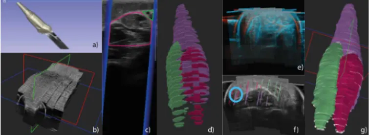
1) Dataset acquisition: In collaboration with Crouzier et.al. [43], 3D-US recordings of 44 participants were collected. Volunteers aged between 18 and 45 years old were prone with their leg in a custom made bath to prevent pressure dependency in the measure. A total of 59 acquisitions were taken, 15 legs were recorded twice with different setting parameters to assure correct and complete visualization of the muscles. Four to six parallel sweeps were performed from the knee to the ankle (Fig. 6 b), under optical tracking of the probe (Fig 6 a). Images were recorded every 5 mm in low speed mode. High resolution 3D ultrasound volumes are compounded using the tracking matrices of the probe, filling a voxel grid of
AUTHOR et al.: PREPARATION OF PAPERS FOR IEEE TRANSACTIONS ON MEDICAL IMAGING 7
a)
a) b) c) d) f)
e)
g)
Fig. 6. 3D-US dataset: a) Tracked US probe b) 5 B-mode image sweeps
c) B-mode image with stradwin mask seeds of muscles d) GM in pink, GL in green and SOL in purple e) Misaligned US volumes f) Misaligned seeds g) Volume created after registration, label interpolation and pol-ishing with seeds representation in white.
564 × 632 × 1443 ± (49 × 38 × 207), with an average isotropic voxel spacing of 0.276993 mm ± 0.015 mm.
2) Mask annotations: Segmentation labels of GM, GL and SOL muscles were first approximated through interpolation of the seeds (Fig 6 d). The “Partial sparse seeds” were created over 2D B-mode US images using the Stradwin [44] software (Fig 6 c). After computing the error between the interpolated approximation and the fully manual slice by slice segmentation of 10 volumes (volumetric error of 4,17%, Dice of 9% and a mIoU of 14.3%) we concluded interpolation alone was not reliable to train a learning method. Therefore, manual polishing by an expert was done over the interpolated volumes, leaving only 2 uncorrected and noisy approximations which we still use in the validation set.
For patients with 2 recordings, GM and GL seeds are done over the first acquisition (r1) while SOL seeds are done over
the second one (r2) with more gain and less frequency. We rely
on 3D-3D image-based rigid registration to combine labels from different ultrasound acquisitions of the same muscle with different qualities (Fig 6 e-g). As a result, we obtain a complete segmentation of the 3 muscles over the volume reconstructed from acquisition r1.
3) Dataset splits: In this study, our data split is done in a patient-wise manner. Out of the acquisitions of the 44 partici-pants, 29 sequences with around 29 × 1400 = 40600 images are used for training. Those sequences are cropped and padded on volumes of size 512 × 512 × 1400 ± 207 to keep the voxel spacing unchanged. The GM, GL and SOL muscles are provided over a single volume. For validation and test set, we use the data of the remaining 5 and 10 participants with around 7000 and 14000 images, respectively.
B. Evaluation Metrics
For assessing the segmentation outcome we compute the Dice similarity coefficient (Dice) and the mean Intersection over Union (mIoU). However, to quantify the smoothness and the surface error of the predicted binary volume, Hausdorff Distance (HDD in mm) and Average Surface Distance (ASD in mm) were evaluated. We also report Precision (P) and Recall (R) to show their trade-off and highlight the importance of using the parametric Tversky loss. All the metrics are reported over the validation and the test set. Finally, toward assessing volume measurements, which is our ultimate goal,
we compute the volume of each of the SOL, GL and GM muscles and report the percentage of error with respect to the ground-truth binary volume.
To calculate the volume of the segmented muscles, the total number of pixels located inside the masks are added, consider-ing the voxel spacconsider-ing (vs). In this study, we have an average isotropic voxel spacing of 0.276993 mm × 0.276993 mm × 0.276993 mm, that varies from one participant to another with a standard deviation of ± 0.015 mm.
C. Methods Comparison
Our evaluation is divided into 2 parts. In the first part, we compare both qualitatively and quantitatively, the performance of IFSS-Net using the full supervision mode (IFSS-Net-FS) and the weak supervision mode (IFSS-Net-WS). Then, we compare our volume predictions against a state-of-the-art deep learning propagation method (PG-Net) based on a Siamese Network [19]. Finally, we consider a 3D-Unet with full supervision as a baseline. All methods are reported over the validation and test data. In the second part of the evaluation, we compare our methods to non-learning segmentation based methods, both qualitatively and quantitatively. We used the Slicer 3D open-source software [45] with built-in algorithms that propagate masks from initial reference annotations. We specifically use: “Fill Between Slices (FBS)”, “Grow from seeds (GFS)” and “Watershed (WS)” methods.
1) IFSS-Net performance: We assessed the segmentation performance (i.e. Dice, mIoU, HDD, ASD, P and R) and study the impact on the final volume computation (i.e. V). Fig. 8 and Fig. 9 show the obtained metrics for the four segmentation methods over the validation and test set re-spectively. Fig. 10 shows the average error (in percentage) of the computed muscle volumes starting from the predicted segmentations.
3D-UNET Watershed PG-Net
Ground Truth IFSS-NET-WS IFSS-NET-FS
Fig. 7. Predicted volume of GM (pink), GL (green) and SOL (violet)
volumes over four methods for one test patient.
The best measures were achieved in case of the IFSS-Net in full supervision mode (IFSS-Net-FS) reporting over the three muscles an average of: 0.9872 ± 0.0016 Dice, 0.977 ± 0.0047 mIoU, 0.578 ± 0.039 mm HDD and 0.197 ± 0.026 mm ASD. The HDD and the ASD measures determine the surface smoothness of the segmented muscle, lower scores indicate better segmentation quality. Fig. 7 shows for “IFSS-Net-FS” a very smooth prediction and a closer to the ground truth segmentation yielding to a small % of volume error with 1.2315 ± 0.465 as an average over the validation and the test set. IFSS-Net-FS is then followed by IFSS-Net-WS, which is trained in weak supervision mode, reporting over the three muscles an average of: 0.985 ± 0.004 Dice, 0.971 ± 0.006
mIoU, 0.728 ± 0.084 mm HDD and 0.275 ± 0.031 mm ASD. IFSS-Net-WS yields to a % of volume error of 1.6035±0.587. The weakly supervised prediction, as shown in Fig. 7, is also smooth and achieves competitive performance to IFSS-Net-FS. PG-Net is in the third place, in term of Dice and mIoU measures, however, it performs a segmentation similar to zero-order interpolation as shown in Fig. 7, yielding to an unsmooth volume surface prediction. Therefore, PG-Net reported high HDD 18.407 ± 0.13 mm and 7.126 ± 0.16 mm ASD scores, while yielding to 18.617 ± 3.984 % of volume error. In comparison with the PG-Net, the 3D-Unet achieves the lower Dice 0.767 ± 0.149 and 0.678 ± 0.137 mIoU. However, the 3D-Unet results in smoother predictions than PG-Net, as shown in Fig. 7, and also achieves better HDD and ASD, 13.374 ± 0.125 mm and 5.46 ± 0.18 mm respectively. Thus, the 3D-Unet provides lower volume errors than PG-Net (13.013 ± 2.84105 % ), but much higher than our IFSS-Net methods. IFS S-N et-WS IFS S-N et-FS 3D -Unet PG-Net 0.7 0.8 0.9 1
Dice Similarity Coefficient
IFS S-N et-WS IFS S-N et-FS 3D -Unet PG-Net 0.6 0.8 1 SOL GL GM mIoU IFS S-N et-WS IFS S-N et-FS 3D -Unet PG-Net 0 2 4 6 8
Average Surface Distance
IFS S-N et-WS IFS S-N et-FS 3D -Unet PG-Net 0 5 10 15 20 HDD IFS S-N et-WS IFS S-N et-FS 3D -Unet PG-Net 0.6 0.7 0.8 0.9 1 Precision IFS S-N et-WS IFS S-N et-FS 3D -Unet PG-Net 0.85 0.9 0.95 1 Recall
Fig. 8. Overview of metrics for the different segmentation methods over
validations set.
Regarding our IFSS-Net-WS, we visualize the surface error map over GL, GM and SOL to analyze if the muscles were equally difficult to segment. Fig. 11 shows the distance to the ground truth in color for each muscle. The values go from 0 mm until 2, 07 mm. We can see that SOL muscle is the hardest to segment. Highlighted sub-volume regions in red are for the most part explained by the poor quality of the US images in those regions. For GM and GL, the endpoints were harder to segment, while not surpassing 0, 52 mm of distance error. This might be due to our model failing to propagate the masks until the muscle endpoints as the US sub-volume become noisy. Our results are supported by Fig. 8 and Fig. 9. Fig. 8 and Fig. 9 also report the precision and recall for each of the methods over the validation and the test set. Here, we show that the trade-off between P and R is better achieved with IFSS-Net using the parametric Tversky loss, indicating a successful segmentation. However, when the Dice loss is used, the curves tend to have higher R and lower P, yielding to lower
IFS S-N et-WS IFS S-N et-FS 3D -Unet PG-Net 0.8 0.85 0.9 0.95 1
Dice Similarity Coefficient
IFS S-N et-WS IFS S-N et-FS 3D -Unet PG-Net 0.7 0.8 0.9 1 SOL GL GM mIoU IFS S-N et-W S IFS S-N et-FS 3D -Unet PG-Net 0 2 4 6
Average Surface Distance
IFS S-N et-WS IFS S-N et-FS 3D -Unet PG-Net 0 5 10 HDD IFS S-N et-WS IFS S-N et-FS 3D -Unet PG-Net 0.6 0.8 1 Precision IFS S-Net-W S IFS S-Net-F S 3D -Unet PG-Net 0.95 1 Recall
Fig. 9. Overview of metrics for the different segmentation methods over
test set.
IFSS-Net-WS IFSS-Net-FS 3D-Unet PG-Net
0 5 10 15 20 25 SOL-Val SOL-Test GL-Val GL-Test GM-Val GM-Test
% of volume error fraction
Fig. 10. Overview of % volume error fraction for the different
segmen-tation methods.
segmentation performances, as it is the case of 3D-Unet and PG-Net.
Fig. 12 shows the full distribution of the HDD and ASD scores at different levels for the SOL muscle over the test set. For each patient volume, this plot shows where are most of the values are concentrated, giving information about the distribution of the variance. Starting with the HDD scores, we can see that IFSS-Net-FS and IFSS-Net-WS are between 0 and 1.024. For 3D-Unet, we can see that for the test patients “P35, P37, P39, P41, and P43”, the HDD distribution scores are less than 10 mm and most of the HDD scores are concentrated between 0 mm 4 mm with a small variance. These results suggest that most of the slices report a score close to their mean value. However, for patients “P36, P38, P40, P42, and P44” HDD scores over slices are above 15 mm and up to 50 mm but still showing small variance. For PG-Net, the variance is higher than 3D-Unet or IFSS-Net, reporting a flat curve. This means that PG-Net is having difficulty to propagate the reference mask while going in depth, leading to higher HDD scores over slices as it goes away from the reference mask. If we look in particular to patients “P35, P37, P39, P41, and P43”, many of the HDD scores over the slices are above
AUTHOR et al.: PREPARATION OF PAPERS FOR IEEE TRANSACTIONS ON MEDICAL IMAGING 9 0 2.07 1.57 1.05 0.52 mm GL GM SOL
Fig. 11. Surface error map for IFSS-Net-WS.
Fig. 12. HDD and ASD scores distribution over the test set for the
different segmentation methods for SOL muscle.
the mean values. PG-Net, has similar difficulties segmenting some patients as the 3D-Unet. In a similar manner, the full distribution of ASD scores is presented in Fig. 12, showing that PG-Net achieved a flat uniform variance over each patient volume. We can see that our network IFSS-Net is well behaved having low scores with very small variance close to 0.389 in both full and weak supervision mode.
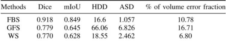
2) Non-learning Mask Based Propagation Methods:We per-form a comparison with other popular non-learning interactive segmentation methods using 3.5% range of binary masks as seeds. We follow approximately similar experimental protocol setting to IFSS-Net, however here each 100 slices, we provide 3 binary annotated masks as seeds. FBS method does prop-agation over binary label masks only. It is an iterative mor-phological contour interpolator method that creates gradual change in the object. GFS and WS methods take into account the image content on top of the label-seeds. In addition to enforcing a smooth transition between the annotated slices, they push the segmented region’s boundaries to coincide with the image contours. Most of our compared built-in approaches assume homogeneous areas of interest and well-defined image contours. Despite the competitive performance in other modal-ities, the assumptions above do not hold in the case of muscles in 3D US images, resulting in leakage. Without a specialized modification, the simple built-in implementation requires a large amount of labeled background and foreground seeds. The application of FBS, GFS and WS methods on our dataset leads to the metrics reported in Table I. FBS gets a higher volumetric error than WS, because it depends on the closeness of the annotations to the edge. However, although WS has leakage, it has better volume estimation. In comparison to our IFSS-Net method, our network has learned to adapt to complex volume structure and to learn properly the shape properties over the entire volume, providing a better volume estimation while avoiding the weakness of FBS, GFS and WS.
Qualitative results in Fig. 7 evidence the daily challenges that experts are faced with when providing manual annotations for ultrasound images. The lack of well-defined edges and the little contrast between regions of interest makes it difficult to
define the segmentation mask borders.
TABLE I
NON-LEARNING MASK BASED PROPAGATION METHODS EVALUATION FOR MUSCLE SEGMENTATION IN3D USSCANS.
Methods Dice mIoU HDD ASD % of volume error fraction
FBS 0.918 0.849 16.6 1.057 10.78
GFS 0.779 0.645 66.06 6.826 16.71
WS 0.770 0.628 18.55 2.462 6.80
V. CONCLUSION
In this paper, we proposed a new approach merging the benefits from expert interactions and deep-learning, dedi-cated to sequential or volumetric data. We deploy several strategies (Siamese network with subvolume recurrency, Bi-CLSTM, 3D ACS and pseudo-labelling) to exploit the spatio-temporal coherence of such data. The resultant IFFS-Net, allows propagating few-reference annotations over the entire volume/sequence while minimizing the expert efforts during training. We presented an in-depth evaluation of the muscle segmentation and volume estimation tasks in 3D freehand ultrasound volumes.
One of the perspectives of this work is the validation of our IFSS-Net over 3D freehand US volumes coming from children with Duchenne Muscular Dystrophy. With the disease progres-sion, muscles become harder to segment as they are replaced by fatty tissues. Hence, some adaptions will be required. One solution would be to fine-tune over a small set of DMD patients or train the network on other domain that contain fatty tissues. Another solution would be to adapt the well known classification zero-shot learning paradigm for segmentation purposes. The usability of our proposed methodology may also be useful for the segmentation other anatomies requiring volume measurements and for other medical image analysis tasks dealing with sequential data.
REFERENCES
[1] Pichiecchio, A., Alessandrino, F., Bortolotto, C., Cerica, A., Rosti, C., Raciti, M.V., Rossi, M., Berardinelli, A., Baranello, G., Bastianello, S., et al.: Muscle ultrasound elastography and mri in preschool children with duchenne muscular dystrophy. Neuromuscular Disorders 28(6), 476–483 (2018)
[2] M. Dunnhofer, M. Antico, F. Sasazawa, Y. Takeda, S. Camps, N. Mar-tinel, C. Micheloni, G. Carneiro, and D. Fontanarosa, “Siam-u-net: encoder-decoder siamese network for knee cartilage tracking in ultra-sound images,” Medical Image Analysis, vol. 60, p. 101631, 2020. [3] R. Zhou, W. Ma, A. Fenster, and M. Ding, “U-net based automatic
carotid plaque segmentation from 3d ultrasound images,” in Medical Imaging 2019: Computer-Aided Diagnosis, vol. 10950. International Society for Optics and Photonics, 2019, p. 109504F.
[4] R. J. Crawford, J. Cornwall, R. Abbott, and J. M. Elliott, “Manually defining regions of interest when quantifying paravertebral muscles fatty infiltration from axial magnetic resonance imaging: a proposed method for the lumbar spine with anatomical cross-reference,” BMC musculoskeletal disorders, vol. 18, no. 1, p. 25, 2017.
[5] J. M. Elliott, D. M. Courtney, A. Rademaker, D. Pinto, M. M. Sterling, and T. B. Parrish, “The rapid and progressive degeneration of the cervical multifidus in whiplash: a mri study of fatty infiltration,” Spine, vol. 40, no. 12, p. E694, 2015.
[6] A. Karlsson, O. D. Leinhard, U. ˚Aslund, J. West, T. Romu, ¨O. Smedby, P. Zsigmond, and A. Peolsson, “An investigation of fat infiltration of the multifidus muscle in patients with severe neck symptoms associated with chronic whiplash-associated disorder,” Journal of Orthopaedic & Sports Physical Therapy, vol. 46, no. 10, pp. 886–893, 2016.
[7] J. M. Morrow, C. D. Sinclair, A. Fischmann, P. M. Machado, M. M. Reilly, T. A. Yousry, J. S. Thornton, and M. G. Hanna, “Mri biomarker assessment of neuromuscular disease progression: a prospective obser-vational cohort study,” The Lancet Neurology, vol. 15, no. 1, pp. 65–77, 2016.
[8] J. A. Noble and D. Boukerroui, “Ultrasound image segmentation: a survey,” IEEE Transactions on medical imaging, vol. 25, no. 8, pp. 987– 1010, 2006.
[9] H. Chen, D. Ni, J. Qin, S. Li, X. Yang, T. Wang, and P. A. Heng, “Stan-dard plane localization in fetal ultrasound via domain transferred deep neural networks,” IEEE Journal of Biomedical and Health Informatics, vol. 19, no. 5, pp. 1627–1636, 2015.
[10] S. Han, H.-K. Kang, J.-Y. Jeong, M.-H. Park, W. Kim, W.-C. Bang, and Y.-K. Seong, “A deep learning framework for supporting the classifi-cation of breast lesions in ultrasound images,” Physics in Medicine & Biology, vol. 62, no. 19, p. 7714, 2017.
[11] B. Schmauch, P. Herent, P. Jehanno, O. Dehaene, C. Saillard, C. Aub´e, A. Luciani, N. Lassau, and S. J´egou, “Diagnosis of focal liver lesions from ultrasound using deep learning,” Diagnostic and interventional imaging, vol. 100, no. 4, pp. 227–233, 2019.
[12] R. J. Cunningham, P. J. Harding, and I. D. Loram, “Real-time ultra-sound segmentation, analysis and visualisation of deep cervical muscle structure,” IEEE transactions on medical imaging, vol. 36, no. 2, pp. 653–665, 2016.
[13] A. Zhao, G. Balakrishnan, F. Durand, J. V. Guttag, and A. V. Dalca, “Data augmentation using learned transformations for one-shot medical image segmentation,” in Proceedings of the IEEE conference on com-puter vision and pattern recognition, 2019, pp. 8543–8553.
[14] X. Zheng, Y. Wang, G. Wang, and J. Liu, “Fast and robust segmentation of white blood cell images by self-supervised learning,” Micron, vol. 107, pp. 55–71, 2018.
[15] ´A. S. Hervella, J. Rouco, J. Novo, and M. Ortega, “Retinal image un-derstanding emerges from self-supervised multimodal reconstruction,” in International Conference on Medical Image Computing and Computer-Assisted Intervention. Springer, 2018, pp. 321–328.
[16] V. Gonzalez Duque, D. AL CHANTI, M. Crouzier, A. Nordez, L. La-courpaille, and D. Mateus, “Spatio-temporal Consistency and Negative Label Transfer for 3D freehand US Segmentation,” in the 23rd Interna-tional Conference on Medical Image Computing and Computer Assisted Intervention,, Lima, Peru, Oct. 2020.
[17] L. Chen, P. Bentley, K. Mori, K. Misawa, M. Fujiwara, and D. Rueck-ert, “Self-supervised learning for medical image analysis using image context restoration,” Medical image analysis, vol. 58, p. 101539, 2019. [18] O. Petit, N. Thome, A. Charnoz, A. Hostettler, and L. Soler, “Handling missing annotations for semantic segmentation with deep convnets,” in Deep Learning in Medical Image Analysis and Multimodal Learning for Clinical Decision Support. Springer, 2018, pp. 20–28.
[19] S. Wug Oh, J.-Y. Lee, K. Sunkavalli, and S. Joo Kim, “Fast video object segmentation by reference-guided mask propagation,” in Proceedings of the IEEE conference on computer vision and pattern recognition, 2018, pp. 7376–7385.
[20] R. Tao, E. Gavves, and A. W. Smeulders, “Siamese instance search for tracking,” in Proceedings of the IEEE conference on computer vision and pattern recognition, 2016, pp. 1420–1429.
[21] L. Bertinetto, J. Valmadre, J. F. Henriques, A. Vedaldi, and P. H. Torr, “Fully-convolutional siamese networks for object tracking,” in European conference on computer vision. Springer, 2016, pp. 850–865. [22] D. Held, S. Thrun, and S. Savarese, “Learning to track at 100 fps with
deep regression networks,” in European Conference on Computer Vision. Springer, 2016, pp. 749–765.
[23] J. Valmadre, L. Bertinetto, J. Henriques, A. Vedaldi, and P. H. Torr, “End-to-end representation learning for correlation filter based tracking,” in Proceedings of the IEEE Conference on Computer Vision and Pattern Recognition, 2017, pp. 2805–2813.
[24] A. Gomariz, W. Li, E. Ozkan, C. Tanner, and O. Goksel, “Siamese networks with location prior for landmark tracking in liver ultrasound sequences,” in 2019 IEEE 16th International Symposium on Biomedical Imaging (ISBI 2019). IEEE, 2019, pp. 1757–1760.
[25] Y.-T. Hu, J.-B. Huang, and A. Schwing, “Maskrnn: Instance level video object segmentation,” in Advances in neural information processing systems, 2017, pp. 325–334.
[26] F. Perazzi, A. Khoreva, R. Benenson, B. Schiele, and A. Sorkine-Hornung, “Learning video object segmentation from static images,” in Proceedings of the IEEE conference on computer vision and pattern recognition, 2017, pp. 2663–2672.
[27] A. Khoreva, R. Benenson, E. Ilg, T. Brox, and B. Schiele, “Lucid data dreaming for object tracking,” in The DAVIS Challenge on Video Object Segmentation, 2017.
[28] Q. Liu, F. Zhou, R. Hang, and X. Yuan, “Bidirectional-convolutional lstm based spectral-spatial feature learning for hyperspectral image classification,” Remote Sensing, vol. 9, no. 12, p. 1330, 2017. [29] L.-C. Chen, Y. Zhu, G. Papandreou, F. Schroff, and H. Adam,
“Encoder-decoder with atrous separable convolution for semantic image segmen-tation,” in Proceedings of the European conference on computer vision (ECCV), 2018, pp. 801–818.
[30] P. O. Pinheiro, T.-Y. Lin, R. Collobert, and P. Doll´ar, “Learning to refine object segments,” in European conference on computer vision. Springer, 2016, pp. 75–91.
[31] D.-H. Lee, “Pseudo-label: The simple and efficient semi-supervised learning method for deep neural networks,” in Workshop on challenges in representation learning, ICML, vol. 3, no. 2, 2013.
[32] J. Enguehard, P. O’Halloran, and A. Gholipour, “Semi-supervised learning with deep embedded clustering for image classification and segmentation,” IEEE Access, vol. 7, pp. 11 093–11 104, 2019. [33] K. Wang, D. Zhang, Y. Li, R. Zhang, and L. Lin, “Cost-effective active
learning for deep image classification,” IEEE Transactions on Circuits and Systems for Video Technology, vol. 27, no. 12, pp. 2591–2600, 2016. [34] Y. Bengio, J. Louradour, R. Collobert, and J. Weston, “Curriculum learning,” in Proceedings of the 26th annual international conference on machine learning, 2009, pp. 41–48.
[35] C. H. Lin, M. Mausam, and D. S. Weld, “Re-active learning: Active learning with relabeling.” in AAAI, 2016, pp. 1845–1852.
[36] C. H. Sudre, W. Li, T. Vercauteren, S. Ourselin, and M. J. Cardoso, “Generalised dice overlap as a deep learning loss function for highly unbalanced segmentations,” in Deep learning in medical image analysis and multimodal learning for clinical decision support. Springer, 2017, pp. 240–248.
[37] S. S. M. Salehi, D. Erdogmus, and A. Gholipour, “Tversky loss function for image segmentation using 3d fully convolutional deep networks,” in International Workshop on Machine Learning in Medical Imaging. Springer, 2017, pp. 379–387.
[38] P. J. Werbos, “Backpropagation through time: what it does and how to do it,” Proceedings of the IEEE, vol. 78, no. 10, pp. 1550–1560, 1990. [39] D. Tran, L. Bourdev, R. Fergus, L. Torresani, and M. Paluri, “Learning spatiotemporal features with 3d convolutional networks,” in Proceedings of the IEEE international conference on computer vision, 2015, pp. 4489–4497.
[40] K. He, X. Zhang, S. Ren, and J. Sun, “Identity mappings in deep residual networks,” in European conference on computer vision. Springer, 2016, pp. 630–645.
[41] C. Peng, X. Zhang, G. Yu, G. Luo, and J. Sun, “Large kernel matters– improve semantic segmentation by global convolutional network,” in Proceedings of the IEEE conference on computer vision and pattern recognition, 2017, pp. 4353–4361.
[42] D. P. Kingma and J. Ba, “Adam: A method for stochastic optimization,” in International Conference on Learning Representations, 2014. [43] M. Crouzier, L. Lacourpaille, A. Nordez, K. Tucker, and F. Hug,
“Neuromechanical coupling within the human triceps surae and its consequence on individual force-sharing strategies,” Journal of Experi-mental Biology, vol. 221, no. 21, 2018.
[44] G. Treece, R. Prager and A. Gee Cambridge University, “Stradwin v6.02,” (2020).
[45] A. Fedorov, R. Beichel, J. Kalpathy-Cramer, J. Finet, J.-C. Fillion-Robin, S. Pujol, C. Bauer, D. Jennings, F. Fennessy, M. Sonka et al., “3d slicer as an image computing platform for the quantitative imaging network,” Magnetic resonance imaging, vol. 30, no. 9, pp. 1323–1341, 2012.

![Fig. 4. Global feature matching layer g with enlarged receptive field by combining [w × 1 × 1] + [1 × f × 1] + [1 × 1 × f] and [w × 1 × 1] + [1 × 1 × f] + [1 × f × 1] convolution layers.](https://thumb-eu.123doks.com/thumbv2/123doknet/11570194.297489/6.918.78.444.81.165/global-feature-matching-enlarged-receptive-combining-convolution-layers.webp)