Ultraviolet auroral emissions
on giant planets
Denis Grodent
[1]
Bertrand Bonfond
[1]
, Aikaterini Radio3
[1]
,
Jacques Gus3n
[1]
, Jean-Claude Gérard
[1]
,
Maïté Dumont
[1]
, Benjamin Palmaerts
[1,2]
[1] Laboratoire de Physique Atmosphérique et Planétaire, Université de Liège, Belgium
[2] Max-Planck-InsGtut für Sonnensystemforschung, GöMngen, Germany
1
[email protected]
ESWW12 – Oostende, 25 Nov 2015
CollecGon of 7 review papers
previously published in Space
Science Reviews
focus on space weather
perspecGve:
Delamere et al. 2015
"Solar wind and internally driven
dynamics"
Grodent 2015
"Brief review of UV auroral emissions
on giant planets"
Springer 2016
Earth ≠ Jupiter ≠ Saturn
magnetospheres - aurorae
Jupiter UV aurora
H
2
Lyman-Werner, Ly-
α
HST – ACS FUV images
Polar S3 map
rotaGng with planet
5
[email protected]
Saturn UV
aurora
H
2
Lyman-Werner
Ly-
α
Sun
Cassini UVIS
FUV "images"
Polar LT map
RotaGng
magnetosphere
Fran Bagenal
7
[email protected]
6
M.G. Kivelson
Table 1 Radii, Sidereal Rotation Periods, and Dominant Magnetospheric Ions of Selected Planets
∗
Planet/Property
Equatorial radius (km)
Rotation period (h)
Dominant ions
Earth
6,378
23.934
H
+
Jupiter
71,492
9.925
O
+
, O
++
, S
+
, S
++
,
S
+++
Saturn
60,268
10.543
∗∗
Water group ions
∗
Radii from Davies et al. (
1996
), rotation periods from de Pater and Lissauer (
2010
)
∗∗
The internal rotation period of Saturn is not known. This value is based on indirect evidence
the mass of typical plasma ions is an order of magnitude larger than the mass of the
pro-tons that normally dominate terrestrial plasmas. Consequently inertial effects are far more
important at Jupiter and Saturn than at Earth. Furthermore the large spatial dimensions and
rapid rotation of the giant planets (see Table
1
) mean that the solar wind flows past only a
portion of these magnetospheres in one planetary rotation period. Interaction with the solar
wind does not dominate their dynamics. Magnetospheric and ionospheric plasmas interact
through signals carried through the system by magnetohydrodynamic (MHD) waves, and
the large travel distances through the giant planet magnetospheres introduce phase delays
that are not readily recognizable at Earth. Furthermore, the plasma density drops rapidly as
one follows a flux tube from the equator to the ionosphere, inhibiting the coupling of
dif-ferent parts of the system. Indeed, the outer parts of these magnetospheres may be unable
to communicate with their ionospheres. Rapid rotation of the heavy ion plasma modifies the
geometry and dynamics of the entire magnetosphere and controls aspects of plasma heating
and loss through mechanisms that differ from processes significant at Earth.
Schematic illustrations of magnetospheres typically depict the field and plasma in a
noon-midnight cut such as shown for Jupiter in Fig.
1
. To a considerable degree, such a cartoon
image can be viewed as generic, an approximate representation of any planetary
magneto-sphere. There is an upstream shock, a magnetosheath in which the diverted solar wind flows
around a boundary that confines most of the field lines that emerge from the planet. A few
of those field lines do not close back on the planet but link directly to the solar wind. In the
anti-solar direction, there is a stretched magnetotail centered on a region of high plasma and
current density, the plasma sheet. Field lines threading the low density region are probably
connected to the solar wind. Of fundamental significance to the discussion of this paper is
a feature absent at Earth. At Jupiter and at Saturn field lines are stretched at the equator not
only on the night side, as at Earth, but also on the day side. This type of field distortion
implies the presence of radially extended azimuthal currents flowing on both day and night
sides of the planet. The current-carrying region embedded in relatively dense plasma that is
confined near the equatorial plane at a large range of local times is what we here refer to as
a magnetodisc.
This book is dedicated to describing the properties of the magnetodiscs of Jupiter and
Saturn and interpreting their interactions with remote parts of the magnetosphere/ionosphere
system. To set the stage for the discussion, this chapter discusses the origin of the disk-like
structure and identifies some problems in the most basic interpretations of their structure.
2 Magnetodisc Formation
Magnetodiscs form in the rotating magnetized plasmas of planetary magnetospheres. Close
to a planet, the currents that generate the magnetic field (dominated by the dipolar
con-Important centrifugal effects at Jupiter and Saturn
FormaGon of a complete magnetodisc
Io
Enceladus, rings
SW
Kivelson, 2015
Fran Bagenal & Steve Bartlej
Enceladus
cryo-volcanism
9
[email protected]
Effect of the solar wind (space weather)
Fran Bagenal & Steve Bartlej
At Jupiter and Saturn field lines are
stretched in the equatorial plane
also on the dayside
⟹ radially extended azimuthal
currents ⟹ magnetodisc
Russell et al., 1982
Effect of the Solar Wind (Space Weather)
Solar Wind characterisGcs (vs distance)
Sonic-Alfvénic
Mach number
electron density
B field
Plasma β
Spiral angle θ
dist. AU
11
[email protected]
SLAVIN ET AL.' FLOW ABOUT THE OUTER PLANETS 6281
ship
between
obstacl•
shape
and
bow
shock
shape
under
com-
pa.
rable flow conditions [Spreiter et al., 1966; Slavin et al.,
1983b], there is general consistency
between the two sets of
boundary models. The bow shocks
at Venus and Mars are less
flared than those at the other planets, most probably because
of their lack of strong intrinsic magnetic fields. in general,
ionospheric
obstacles
are not as compressibl
e as dipole mag-
netic fields [Spreiter et al., 1970b; Slavin et al., 1980]. For this
reason,
less flaring at the flanks is .required
for an ion0pause
than for a magnetopause, and this result is reflected in bow
shock shape as shown in Figure 10.
In Figure I 1 the Jupiter
and Saturn
magnetosheath
bound-
aries are compared With the earth results of Slavin and Holzer
[1981]. For this purpose it is necessary
to scale the bow shock
and magnetopause
models to a common dynamic pressure.
Because magnetopause position has been modeled as a func-
tion of indirectly measured dynamic pressure,
Ps,•*, a knowl-
edge of the relationship between Psw and Psw* is required. In
the case of Jupiter, a beta of 1 inside the magnetopause
ap-
pears consistent
with the Voyager particle measurements
[Kri-
migis et al., I981]. The actual dynamic pressure would then be
twice the Psi* value inferred from the magnetic field alone.
This assumption is also supported by the fact that it makes
the average dynamic pressure
during the shock crossings
in
Figure 4 nearly equal to that during the magnetopause
en,
counters in Figure 5. At Saturn, plasma was also detected
within the magnetosphere,
but beta near the magnetopause
appears
to have been
of the order of 10-•, or less
[Krimigis
et
al., 1983; Lanzerotti et al., 1983]. On the basis of these Voy-
ager in situ measurements,
and the sixth-root pressure depen-
dence in Figure 9, we have assumed Ps,• = Ps,•* for Saturn.
Given these assumptions
concerning upstream dynamic pres-
sure, bow shock and magnetopause
boundaries are plotted
250 -
200 -
•o
50-
SOLAR WIND STAND-OFF DISTANCE AT JUPITER
GALILEAN SATELLITES ] .
MEAN
=
68.0 R
N
: 58.6
(1.1
X
10-9/Psw
)1/4
L• N
CALCULATED
=
837
hrs
SERVED 3<>_ • oz '"o60 80 100 lIO 1 0 160
R
N (R
j)
2OO 150 100 50 PIONEER 10 (4.9 - 5.1 AU) _-•.•EI•IA
N
= .
-10
_ I 1 0 4 8 12 N = 837 hrs 18_• 16 20 24 28 32 36 40PSW
(10-10
dY
nes/cm2)
Fig. 12. Histograms of Pioneer 10 solar wind dynamic pressure
measurements
near Jupiter encounter and the corresponding
mag-
netopause positions relative to the Galilean satellites.
PLANETARY
MAGNETOSHEATH
BOUNDARIES
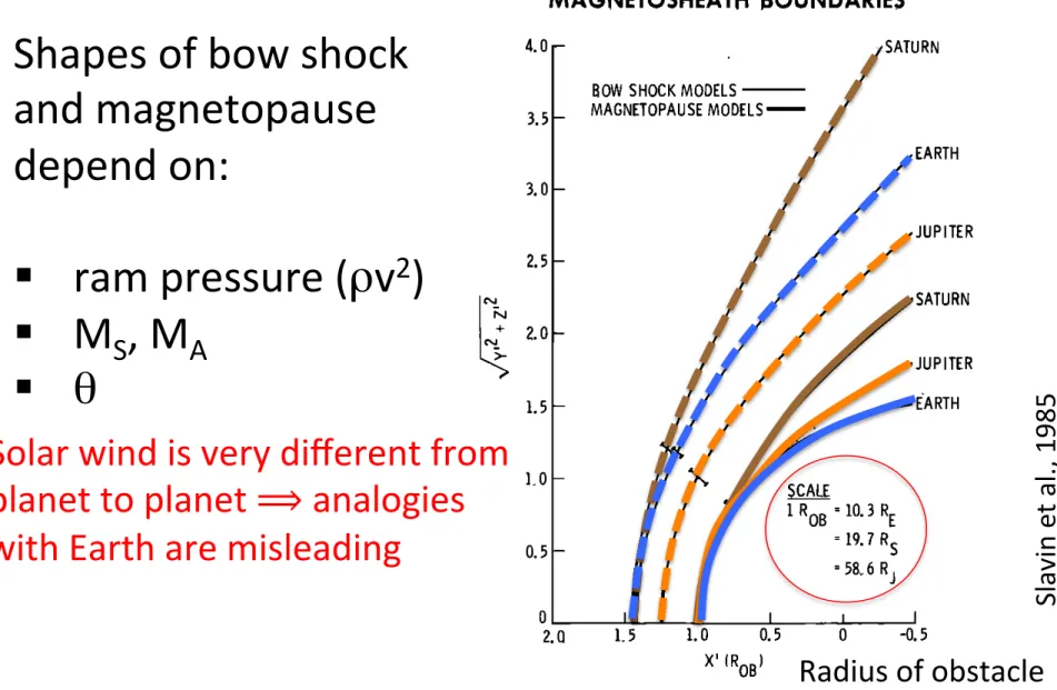
4.0 -- SATURN 3.5 3.0 2.5 + 2.0 1.5 0.5BOW SHOCK MODELS • MAGNETOPAUSE MODELS ' SCALE
1RoB
:10.3R
E
=19.7
R
S
= 58•
6 Rj
EARTH JUPITER RN JUPITERI•ARTH
Fig. 11.
0 i 2.0 1•5 1.0 0.5 0 -0.5X' (ROB)
A comparison of magnetosheath
boundaries at the earth,
Jupiter, and Saturn.
relative to each other for the earth, Jupiter, and Saturn in
Figure 11.
The surfaces
in Figure 11 display two interesting results. At
Jupiter the subsolar
magnetosheath
appears to be much thin-
ner than observed for the earth despite the similar shapes of
their magnetopause boundaries, while the Saturn mag-
netopause is much more flared in shape than those of the
earth or Jupiter. For this reason it would be expected to have
a much thicker magnetosheath
region than these other planets
[e.g., Spreiter et al., 1966; Stahara et al., 1980]. However, the
ratios of subsolar shock to magnetopause
radius are 1.41, 1.25,
and 1.43 at the earth, Jupiter, and Saturn, respectively. In the
sections to follow, these results will be investigated quantita-
tively using gas dynamic model calculations which take into
account both the effects of obstacle shape and Mach number
as a function of distance from the sun.
SOLAR WIND STAND-OFF DISTANCE
Using the magnetopause models and solar wind data sets
described earlier, we have examined the distribution Of solar
wind dynamic pressure and its effect on the distance •to the
nose of the magnetosphere,
Rs. The bottom panels of Figures
12 and 13 display solar wind dynamic pressures
calculated
using the hourly averaged Pioneer 10 and 11 observations
described
earlier. The solid-lined histograms
in the top panels
give the corresponding
magnetopause stand-off distances cal-
culated using the pressure dependences
derived earlier in the
study. As shown in Figure 12, the range in solar wind stand-
off distance at Jupiter is predicted to vary from about 40 Rs to
Radius of obstacle
Shapes of bow shock
and magnetopause
depend on:
§
ram pressure (ρv
2
)
§
M
S
, M
A
§ θ
Sl
av
in
e
t al
.,
19
85
Solar wind is very different from
planet to planet ⟹ analogies
with Earth are misleading
12
[email protected]
SLAVIN ET AL.: FLOW ABOUT THE OUTER PLANETS 6283
4.5 4.0 3.5 3.0 2.5 2.0 1.5 1.0 0.5 SATURN / / / / / / / / GD MODEL M : 12 s H/R = 0.85 o 1 ROB = 19.7 R s 2.0 1.5 1.0 0.5 0 -0.5 X' (ROB)
Fig. 15. Observational models of the Saturnian bow shock and
magnetopause compared with the predictions of high Mach number gas dynamic theory (dashed lines).
blunt sections. The result is a net transfer of mass flux from
the low-latitude magnetosheath, thereby reducing its width, to the high-latitude magnetosheath. The magnitude of the dis- crepancy caused by the assumption of axial symmetry is ex- pected to increase as the degree of polar flattening grows.
In Figure 16 we suggest that the poor agreement between
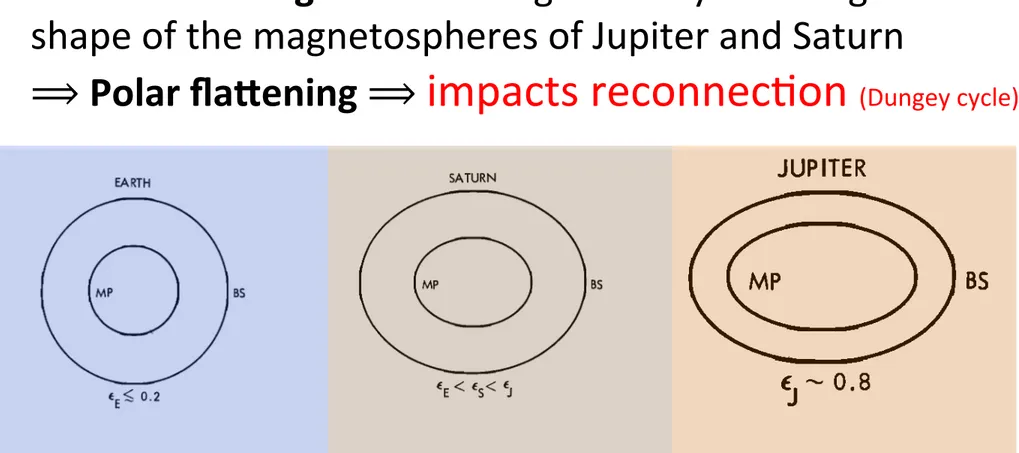
observation and the gas dynamic code, relative to past terres- trial experience, does indeed stem from our assumption of axial symmetry. At the earth, both theory and observation indicate that the eccentricity of the magnetospheric cross sec- tion in the terminator plane is small, ee < 0.2 [Fairfield, 1971; Holzer and Salvin, 1978]. While the higher latitudes at Jupiter
and Saturn have not be examined in situ, theoretical models of
the Jovian field [e.g., Engle and Beard, 1980] suggest consider- POLAR FLATTENING HIERARCHY
JUPITER
BS
SATURN
[1984]). Based upon Table 1 and Figures 1 and 2, sonic Mach
numbers of 10 and 12 were used to represent average con-
ditions at Jupiter and Saturn. The final parameter needed for
the gas dynamic model is the adiabatic exponent 7. On the basis of previous studies [Slavin et al., 1983b], 7 = 2 was used. This value has provided the best agreement between theory and observation with regard to shock position and average flow characteristics at 1 AU.
In Figure 14 it is apparent that the location of the Jovian
bow shock is much closer to the magnetopause than predic- ted. The actual thickness of the Jovian magnetosheath is only 55% of the value predicted by the gas dynamic model. This result is well outside the fitting error bars and much larger than the expected sampling uncertainty based upon the five passes through the subsolar region shown in Figure 3. For Saturn, Figure 15 displays better agreement between the gas dynamic model and observation, but with the predicted sub- solar magnetosheath still about 20% too thin. The poorer
sampling at Saturn may hav e contributed to the discrepancy,
but the overestimate of magnetosheath width by the gas dy- namic model at both planets suggests a common cause pecu- liar to the Jovian and Saturnian solar wind interactions.
In order to interpret these results, we have noted that the
Pioneer and Voyager observational models are based upon moderate- to low-latitude observations. Unlike the case for
the earth, no high-latitude magnetopause and bow shock ob-
servations have been made at Jupiter and Saturn. If Jupiter
and Saturn present non-axially symmetric obstacles to the
solar wind, then a fundamental assumption in our gas dynam-
ic models will no longer hold. The streamlines would cease to
be axially symmetric, with mass flux being channeled from the longer paths about the broad body sections toward the less
BS
•E < •S < •J
EARTH
BS
•E
% 0.2
Fig. 16. A conceptual representation of magnetopause shape in
the terminator plane based upon observations at the earth, theoretical magnetic field models at Jupiter, and interpretation of gas dynamic modeling results.
Presence of magnetodisc is significantly affecGng the
shape of the magnetospheres of Jupiter and Saturn
⟹
Polar fla1ening ⟹
impacts reconnecGon
(Dungey cycle)
SLAVIN ET AL.: FLOW ABOUT THE OUTER PLANETS
6283
4.5
4.0 3.53.0
2.5 2.0 1.5 1.0 0.5 SATURN/
/
/
/
/
/
/ / GD MODEL M : 12 sH/R = 0.85
o1 ROB
= 19.7
R
s
2.0
1.5
1.0
0.5
0
-0.5
X' (ROB)
Fig. 15. Observational models of the Saturnian bow shock and
magnetopause
compared with the predictions of high Mach number
gas dynamic theory (dashed lines).
blunt sections. The result is a net transfer of mass flux from
the low-latitude magnetosheath,
thereby reducing its width, to
the high-latitude magnetosheath.
The magnitude of the dis-
crepancy caused by the assumption of axial symmetry is ex-
pected to increase
as the degree of polar flattening grows.
In Figure 16 we suggest that the poor agreement between
observation and the gas dynamic code, relative to past terres-
trial experience,
does indeed stem from our assumption of
axial symmetry. At the earth, both theory and observation
indicate that the eccentricity
of the magnetospheric
cross sec-
tion in the terminator plane is small, ee < 0.2 [Fairfield, 1971;
Holzer and Salvin, 1978]. While the higher latitudes at Jupiter
and Saturn have not be examined in situ, theoretical models of
the Jovian field [e.g., Engle and Beard, 1980] suggest
consider-
POLAR FLATTENING
HIERARCHY
JUPITER
BS
SATURN
[1984]). Based upon Table 1 and Figures 1 and 2, sonic Mach
numbers of 10 and 12 were used to represent average con-
ditions at Jupiter and Saturn. The final parameter needed for
the gas dynamic model is the adiabatic exponent 7. On the
basis of previous studies [Slavin et al., 1983b], 7 = 2 was used.
This value has provided the best agreement between theory
and observation with regard to shock position and average
flow characteristics at 1 AU.
In Figure 14 it is apparent that the location of the Jovian
bow shock is much closer to the magnetopause
than predic-
ted. The actual thickness
of the Jovian magnetosheath
is only
55% of the value predicted by the gas dynamic model. This
result is well outside the fitting error bars and much larger
than the expected sampling uncertainty based upon the five
passes
through the subsolar region shown in Figure 3. For
Saturn, Figure 15 displays better agreement between the gas
dynamic model and observation,
but with the predicted sub-
solar magnetosheath
still about 20% too thin. The poorer
sampling
at Saturn may hav
e contributed
to the discrepancy,
but the overestimate
of magnetosheath
width by the gas dy-
namic model at both planets suggests
a common cause pecu-
liar to the Jovian and Saturnian solar wind interactions.
In order to interpret these results, we have noted that the
Pioneer and Voyager observational
models are based upon
moderate-
to low-latitude
observations.
Unlike
the case for
the earth, no high-latitude magnetopause
and bow shock ob-
servations
have been made at Jupiter and Saturn. If Jupiter
and Saturn present non-axially symmetric obstacles to the
solar wind, then a fundamental
assumption
in our gas dynam-
ic models will no longer hold. The streamlines would cease to
BS
•E < •S < •J
EARTH
BS
•E
% 0.2
Fig. 16. A conceptual representation
of magnetopause
shape in
the terminator plane based upon observations
at the earth, theoretical
SLAVIN ET AL.: FLOW ABOUT THE OUTER PLANETS 6283
4.5 4.0 3.5 3.0 2.5 2.0 1.5 1.0 0.5 SATURN / / / / / / / / GD MODEL M : 12 s H/R = 0.85 o 1 ROB = 19.7 R s 2.0 1.5 1.0 0.5 0 -0.5 X' (ROB)
Fig. 15. Observational models of the Saturnian bow shock and
magnetopause compared with the predictions of high Mach number gas dynamic theory (dashed lines).
blunt sections. The result is a net transfer of mass flux from
the low-latitude magnetosheath, thereby reducing its width, to the high-latitude magnetosheath. The magnitude of the dis- crepancy caused by the assumption of axial symmetry is ex- pected to increase as the degree of polar flattening grows.
In Figure 16 we suggest that the poor agreement between
observation and the gas dynamic code, relative to past terres- trial experience, does indeed stem from our assumption of axial symmetry. At the earth, both theory and observation indicate that the eccentricity of the magnetospheric cross sec- tion in the terminator plane is small, ee < 0.2 [Fairfield, 1971; Holzer and Salvin, 1978]. While the higher latitudes at Jupiter
and Saturn have not be examined in situ, theoretical models of
the Jovian field [e.g., Engle and Beard, 1980] suggest consider- POLAR FLATTENING HIERARCHY
JUPITER
BS
SATURN
[1984]). Based upon Table 1 and Figures 1 and 2, sonic Mach
numbers of 10 and 12 were used to represent average con-
ditions at Jupiter and Saturn. The final parameter needed for
the gas dynamic model is the adiabatic exponent 7. On the basis of previous studies [Slavin et al., 1983b], 7 = 2 was used. This value has provided the best agreement between theory and observation with regard to shock position and average flow characteristics at 1 AU.
In Figure 14 it is apparent that the location of the Jovian
bow shock is much closer to the magnetopause than predic- ted. The actual thickness of the Jovian magnetosheath is only 55% of the value predicted by the gas dynamic model. This result is well outside the fitting error bars and much larger than the expected sampling uncertainty based upon the five passes through the subsolar region shown in Figure 3. For Saturn, Figure 15 displays better agreement between the gas dynamic model and observation, but with the predicted sub- solar magnetosheath still about 20% too thin. The poorer
sampling at Saturn may hav e contributed to the discrepancy,
but the overestimate of magnetosheath width by the gas dy- namic model at both planets suggests a common cause pecu- liar to the Jovian and Saturnian solar wind interactions.
In order to interpret these results, we have noted that the
Pioneer and Voyager observational models are based upon moderate- to low-latitude observations. Unlike the case for
the earth, no high-latitude magnetopause and bow shock ob-
servations have been made at Jupiter and Saturn. If Jupiter
and Saturn present non-axially symmetric obstacles to the
solar wind, then a fundamental assumption in our gas dynam-
ic models will no longer hold. The streamlines would cease to
be axially symmetric, with mass flux being channeled from the longer paths about the broad body sections toward the less
BS
•E < •S < •J
EARTH
BS
•E
% 0.2
Fig. 16. A conceptual representation of magnetopause shape in
the terminator plane based upon observations at the earth, theoretical magnetic field models at Jupiter, and interpretation of gas dynamic modeling results.
13
[email protected]
DiamagneGc suppression
Large plasma β gradient across a current sheet (magnetopause)
prevents establishment of flow pajerns and B
field
bending required for
reconnecGon (Swisdak et al., 2010)
Flow shear suppression
Super-Alfvénic flow shear in the direcGon of the reconnecGng field can
suppress reconnecGon (Cassak and Ojo, 2011)
Two processes prevent Dungey-like (Earth-like) reconnecGon at Jupiter and Saturn
14
[email protected]
Solar Wind Driven Dynamics
Fig. 4 Assessment of how
favorable conditions at Jupiter’s
magnetopause are for magnetic
reconnection onset. In all panels
the magnetopause surface is
viewed from along the solar wind
flow direction. The panel
surrounded by a blue rectangle
shows an assessment of flow
shear suppression, and the panels
surrounded by a red rectangle
show assessments of diamagnetic
suppression (for different values
of the plasma β in the
magnetosphere, β
MSP
). Regions
of each surface shaded in red are
regions where reconnection onset
is possible. Adapted from
Desroche et al. (
2012
)
across the dawn flank magnetopause generally prohibit reconnection due to flow shear
sup-pression. Furthermore, by considering different values of the (poorly constrained) plasma
β
in Jupiter’s near-magnetopause magnetosphere they showed that diamagnetic suppression
may also be severe.
In the case of Saturn’s magnetosphere, in situ evidence for magnetopause reconnection
has also been reported (Huddleston et al.
1997
; McAndrews et al.
2008
; Lai et al.
2012
;
Fuselier et al.
2014
), and it has been suggested that some dayside auroral features are caused
by bursts of magnetopause reconnection (Radioti et al.
2011a
; Badman et al.
2012a
,
2013
).
However, unlike Jupiter, no examples of FTEs have been identified to date (Lai et al.
2012
),
and neither Saturn’s auroral power nor the thickness on the magnetospheric boundary layer
adjacent to the magnetopause show a clear response to the orientation of the IMF (unlike
Solar Wind Driven Dynamics
Fig. 4 Assessment of how
favorable conditions at Jupiter’s
magnetopause are for magnetic
reconnection onset. In all panels
the magnetopause surface is
viewed from along the solar wind
flow direction. The panel
surrounded by a blue rectangle
shows an assessment of flow
shear suppression, and the panels
surrounded by a red rectangle
show assessments of diamagnetic
suppression (for different values
of the plasma β in the
magnetosphere, β
MSP
). Regions
of each surface shaded in red are
regions where reconnection onset
is possible. Adapted from
Desroche et al. (
2012
)
across the dawn flank magnetopause generally prohibit reconnection due to flow shear
sup-pression. Furthermore, by considering different values of the (poorly constrained) plasma
β
in Jupiter’s near-magnetopause magnetosphere they showed that diamagnetic suppression
may also be severe.
In the case of Saturn’s magnetosphere, in situ evidence for magnetopause reconnection
has also been reported (Huddleston et al.
1997
; McAndrews et al.
2008
; Lai et al.
2012
;
Fuselier et al.
2014
), and it has been suggested that some dayside auroral features are caused
by bursts of magnetopause reconnection (Radioti et al.
2011a
; Badman et al.
2012a
,
2013
).
However, unlike Jupiter, no examples of FTEs have been identified to date (Lai et al.
2012
),
and neither Saturn’s auroral power nor the thickness on the magnetospheric boundary layer
Jupiter
(similar for Saturn)
Flow shear
suppression
DiamagneGc
suppression
ReconnecGon is only possible in the
red regions
Desroche et al., 2012
Masters et al., 2012
Delamere et al., 2013
mtopause of
Jupiter seen
from the Sun
15
[email protected]
P.A. Delamere et al.
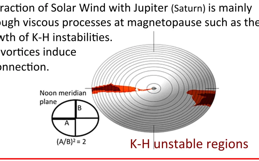
Fig. 6 Assessment of the
stability of Jupiter’s
magnetopause to the growth of
the Kelvin-Helmholtz (K-H)
instability. In all panels the
magnetopause surface is viewed
from along the solar wind flow
direction, and shaded regions of
each surface are regions predicted
to be K-H unstable. Different
panels consider different levels of
magnetospheric polar flattening.
Adapted from Desroche et al.
(
2012
)
processes operating at Jupiter’s magnetopause, limited spacecraft data sets prevent large
statistical analyses. Note that separating wave-driving mechanisms is difficult, i.e. solar wind
pressure fluctuations can cause waves as well as K-H instability growth.
In their assessment of what conditions at Jupiter’s magnetopause mean for how the solar
wind interacts with the magnetosphere, Desroche et al. (
2012
) consider the K-H stability of
the boundary. They found that polar flattening of the magnetosphere (caused by centrifugal
confinement of magnetospheric plasma in roughly the plane of the planetary equator) can
have a significant effect on the flow in the magnetosheath, and that, as expected, the dawn
flank of the magnetopause should be far more K-H unstable than the dusk flank, due to the
difference in flow shears (see Fig.
6
).
Delamere and Bagenal (
2010
) suggested that solar wind driving of Jupiter’s
magneto-sphere is predominantly due to viscous processes, like growth of the K-H instability,
operat-ing at the magnetopause. This model is akin to that of Axford and Hines (
1961
). Delamere
and Bagenal (
2010
) suggested that rather than a global cycle of reconnection where flux is
opened at the dayside magnetopause and closed in the magnetotail, flux is predominantly
opened and closed intermittently in small-scale structures in turbulent interaction regions on
the flanks of the magnetosphere. K-H vortices and associated reconnection is a key element
of this understanding of Jupiter’s magnetospheric dynamics.
Statistical studies of perturbations of Saturn’s magnetopause have provided a clearer
pic-ture of K-H instability growth at this magnetospheric boundary. Case studies initially
re-InteracGon of Solar Wind with Jupiter
(Saturn)
is mainly
through viscous processes at magnetopause such as the
growth of K-H instabiliGes.
K-H vorGces induce
reconnecGon.
K-H unstable regions
Delamere and Bagenal (2010): at Jupiter, flux is predominantly opened and
closed intermijently in small-scale structures in turbulent interacGon
regions (K-H vorGces) on the flanks of the magnetosphere.
Does that mean that at Jupiter and Saturn there
are no SW signatures in the aurora?
Yes and no.
SituaGon is far more complex than at the Earth
because of an addiGonal ingredient: the
subcorotaGng magnetodisc.
17
[email protected]
Jupiter (North)
S3 frame
(equiv. to LT if CML=180°)
Auroral components of giant planets
HST-STIS
GO-12883
Jupiter UV aurora
Northern hemisphere
Grodent, 2015
Saturn (both)
LT frame
"Unshoked"
Aurora
Saturn UV aurora
Southern hemisphere
Cassini -UVIS
DOY 2013-079
alt.:
13.2_12.7 RS
ssc lat:
-49.3°_-47.1°
Auroral components of giant planets
Grodent, 2015
19
[email protected]
Solar Wind Driven Dynamics
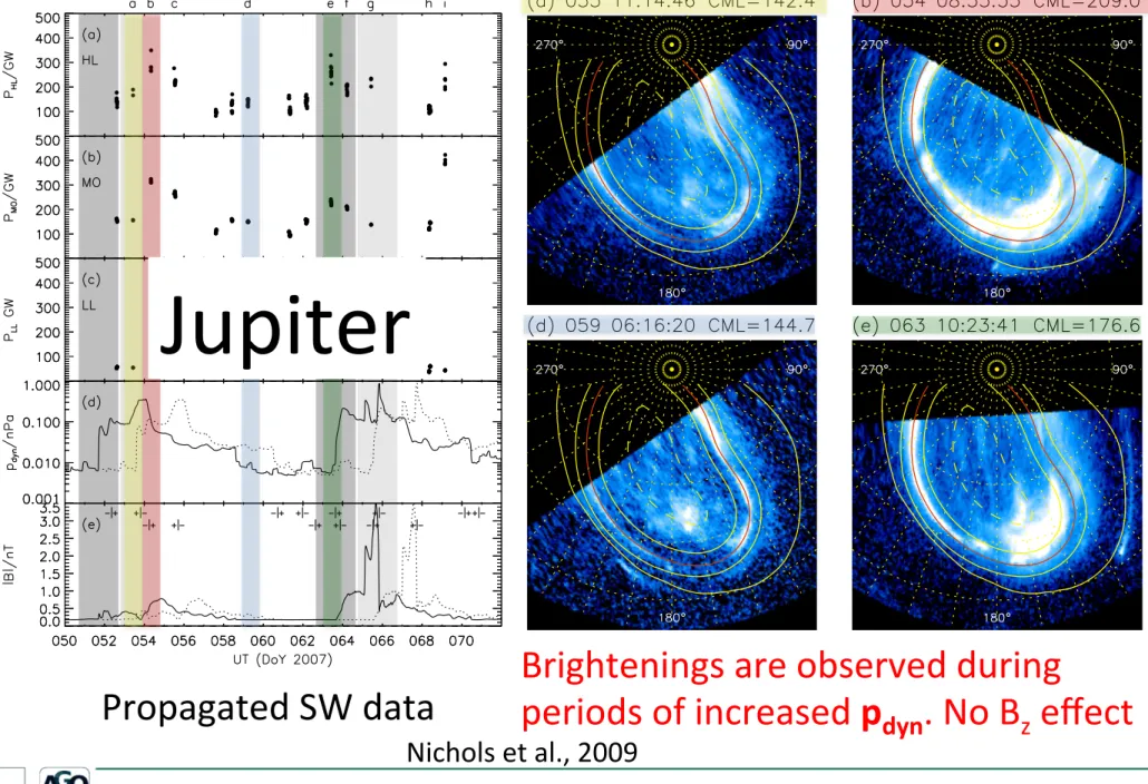
Fig. 16 Representative HST images of Jupiter’s northern auroras corresponding to the visits labeled at the
top of Fig.
15
. The projection view is from above the north pole, and the image is displayed with a log color
scale saturated at 500 kR. The red line shows the reference main oval as given by Table 1 in Nichols et al.
(
2009a
). The solid yellow lines show the boundaries between the high latitude region, the main oval and the
low latitude emission. The dashed yellow line indicates the boundary between the polar inner and polar outer
regions. The yellow points indicate a 10
◦
× 10
◦
planetocentric latitude—SIII longitude grid. The image is
oriented such that SIII longitude 180
◦
is directed toward the bottom. Reproduced from Nichols et al. (
2009a
)
top of Fig.
15
(a) are shown in Fig.
16
. Using these data, Nichols et al. (
2009a
) showed that
Jupiter’s auroras respond to solar wind compression region onset in a broadly repeatable
manner, which can be summarised as follows:
– The total emitted power from the main oval increases by factors of
∼2–3.
– The main oval is brightened along longitudes >165
◦
, and is shifted poleward by
∼ 1
◦
and
expanded, as evidenced in Figs.
16
(b) and (c), and (e–g).
– In contrast, there is little emission at longitudes < 165
◦
, and any auroras are patchy and
disordered.
– Under-sampling notwithstanding, the main oval apparently persists in this disturbed state
for 2–3 days following compression region onset.
Nichols et al., 2009
P.A. Delamere et al.
Fig. 15 Plots showing the power emitted from the different auroral regions, along with the modelled solar
wind conditions for the first HST campaign in February/March 2007. Specifically, we show (a) the power emitted from the high latitude region PHL in GW, (b) the power emitted from the main oval region PMO
in GW, (c) the power emitted from the low latitude region PLLin GW, (d) the solar wind dynamic pressure
in nPa, and (e) the IMF magnitude|B| in nT. The individual points in panels (a)–(c) represent the powers obtained for each image. The solid lines in the MHD model panels show the original model timings, while the dotted line show the timings shifted by+2.1 days. The dark grey regions shows the estimated arrival time of the forward shocks within 1 standard deviation uncertainty of the MHD model timings, and the light
grey regionsare similar but for the shifted timings. Also shown in panel (e) are the estimated locations of the heliospheric sector boundaries, along with the sign of BT either side. The original timing is on top, while the shifted timing is below. Reproduced from Nichols et al. (2009a)