Thermal conductivity of tubular nanowire composites based on a thermodynamical model

1

Thermal conductivity of tubular nanowire composites based on a thermodynamical model

G. Lebon and H. Machrafi*

Thermodynamics of Irreversible Processes, Liège university, 17 Allée du 6 Août, 4000 Liège, Belgium

*Corresponding author

Electronic mails: g.lebon@ulg.ac.be (G.Lebon), h.machrafi@ulg.ac.be (H. Machrafi)

Abstract. A formula for the effective heat conductivity of a nanocomposite with cylindrical nanowire inclusions is derived. Both transversal and longitudinal heating along the wires are investigated. Several effects are examined: the volume fraction and sizes of the nanowires, the type of scattering at the particle-matrix interface and temperature. As illustration, silicon nanowires inclusions in a germanium matrix is considered; the results are shown to be in good agreement with other models and numerical solutions of the Boltzmann transport equation. Our main contribution consists of using extended irreversible thermodynamics to cope with the nano dimensions of the wires.

Keywords: Thermal conductivity; Nanowire composites; Extended thermodynamics; Temperature-dependent phonon properties

2

1. Introduction.

Thermal effects in nanomaterials are the subject of a huge amount of research both from theoretical and technological viewpoints. A question of particular and acute interest is the determination of the effective heat conductivity in nanocomposites. To apprehend the problems, several ways are open: either to solve directly the Boltzmann transport equation [1], to construct phenomenological models [2], to use atomistic simulations [3] or to mix both macroscopic and microscopic considerations which is the route followed in the present approach. More specifically, we consider two-dimensional tubular silicon nanowires embedded in a homogeneous germanium matrix; both cases with the heat flux directed normally and parallel to the axis of the Si wires are investigated To model heat transport in composites, we use a formalism, called the effective medium approximation (EMA), initiated by Nan et al [2] and revisited by Minnich and Chen [4]. Since the dimensions of the nano materials are comparable to the mean free path of the heat carriers, heat transport is mainly of ballistic rather than diffusive nature. Therefore, heat transport can no longer be described by Fourier’s law and classical thermodynamics but requires a more sophisticated approach. Here, we will follow the line of thought of extended irreversible thermodynamics (EIT) which is especially suited to treat problems at sub-scales. The main idea underlying EIT [5,6,7] is to upgrade the thermodynamic fluxes, like the heat flux to the rank of independent variable at the same level as the classical variables, as the temperature. The consequence is that Fourier’s law will be substituted by more complex expressions allowing to deal with high frequency and small-scale systems. EIT has been applied in a previous paper [8] wherein we have studied heat transport in composites formed by spherical particles distributed randomly in a homogeneous matrix. The results were shown to be in good agreement with Monte Carlo simulations and other models [9,10] using different schemes. In the present work, we explore

3

further the applicability and limitations of the model developed in [8] by considering wires instead of spheres because the former play a critical role in a great number of technological applications.

The present paper is organized as follows. The model is set up in section 2. It consists in a mixing of EMA and EIT, whose main ingredients are briefly recalled. In Section 3, the model is applied to the problem of dispersion of Si nanowires in a Ge matrix: influence of volume fractions, size of the nano wires and the thermal boundary resistance are discussed. Temperature dependence of the overall heat conductivity, a topic ignored in most papers, is treated in Section 4. Conclusions are drawn in Section 5.

2. The thermal conductivity model

The basic relation is Maxwell’s one [11] improved by Hasselman and Johnson [12] to include thermal boundary resistance and by Nan et al [2] who considered various particle shapes. Accordingly, the overall thermal conductivity of the composite in the direction perpendicular and normal to the heat flux are respectively given by

0 0 0 0 1 1 1 1 p m p m m p m p m ( ) [( ) ] ( ) [( ) ]                             , (1) 0 (1 ) _{m p} _     . (2) λ0

m is the heat conductivity of the matrix and λp the heat conductivity of the wires. Unlike

λ0

m, the quantity λp will incorporate explicitly size effects as made explicit later on in this

Section 2. Furthermore, φ denotes the volume fraction of the fibers and rK

r

  is a

4

the wire of length L and, rK the so-called Kapitza radius. The latter is expressed by rK= Rλm ,

with R designating the interfacial boundary resistance, given by

1 1 4( _{v v} ) m m p p R c v c v   , (3) where cv

i and vi (i=m, p) are the volumetric specific heats and phonon group velocities

respectively, note that the result (3) was derived by Chen [13] for pure diffusive scattering. Specularity is taken explicitly into account by introducing a “modified” radius r*=(1+s) r /(1-s) and a “modified” length L*=(1+/(1-s)L/(1-/(1-s) wherein the parameter s denotes the probability of specular diffusion of the phonons on the particle–matrix interface; s=0 is characteristic of diffusive collisions (the quantity r* reduces then to r and L* to L) while s=1 denotes pure specular interactions. In the present section and in the next one, we assume that the temperature is fixed, the effects of a variable temperature will be delayed to section 4.

The bulk heat conductivity of the host medium is given by the classical expression

0 1

3 v

m c vm m m T ref

   (4)

where is the reference temperature, say the room temperature. The mean free path Λm of

the phonons inside the matrix is given by the Matthiessen rule:

. (5)

with designating the mean free path in the bulk, is the supplementary

contribution due to the interactions at the particle-matrix interface. Note that although the relation between the mean free path in the matrix and the average separation between

5

neighboring nanowires does not appear explicitly in this formulation, it is implicitly included

in the expression of Λm,coll. In the case of wires with their axis oriented normally and parallel

to the heat flux, this supplementary contribution is given by, respectively, [4,14]: , * 2 1 ,   r coll m   (6)

wherein ζ stands for ζ= √ φ/(√φ+1).

To emphasize the role of the sizeeffects on the heat conductivity λp of the nanowires,

we will write λp in the form

0 S

p p p

   (7)

wherein λp0 contains all the contributions except those linked to the sizes of the nanoparticles

which are described by the correcting factor λpS . The quantity λp0 is given by a relation

similar to (4) with sub-index m substituted by p but wherein Λp refers only to the bulk

contribution as the effects of ballistic collisions will be included in λpS. To determine λpS, we

will refer to EIT whose main idea is to upgrade the thermodynamic fluxes, like the heat flux and higher order fluxes to the rank of independent variables at the same footing as the energy or the temperature.

For the sake of completeness, let us briefly recall the building up of EIT. The first step

consists in assuming that the entropy is not only depending on the internal energy e

but besides on the heat flux vector q so that the corresponding Gibbs equation will be written as

, (8)

6

phenomenological coefficient identified later on. Furthermore, denotes the time derivative. However, expression (8) does not account for non-local effects. To introduce such effects, it is

appealed to a hierarchy of fluxes Q(1)_{, Q}(2)_{, ... Q}(N) _{with Q}(1) _{identified with the heat flux}

vector q, Q(2) _{(a tensor of rank two) is the flux of the heat flux, Q}(3) _{the flux of Q}(2)_{, etc. Up to}

the nth_{-order flux, the Gibbs equation generalizing relation (8) becomes}

, (9)

wherein the symbol  denotes the inner product of the corresponding tensors. The second

step is the formulation of the entropy flux Js_{.It is natural to expect that it is not simply given}

by the classical expression T-1_{q, but that it will depend on higher order fluxes, as}

, (10)

The next step is the derivation of the rate of entropy production per unit volume σs _{which is}

defined by . s s t d     J ≥0, (11)

and is a positive definite quantity according to the second law of thermodynamics. It is

checked that, after substituting in (11) the expressions of dt η and Js from (9) and (10)

respectively and eliminating dt e via the energy conservation law for rigid heat conductors

(d et   q. ), one obtains 1 (2) ( ) ( ) ( 1) ( 1) 1 1 1 2 ( . ). N ( . ) 0 s n n n n t n t n n n T d ... d Q                q Q q 



Q  Q  Q    . (12) The above bilinear expression in fluxes and forces (the quantities between parentheses) suggests the following hierarchy of linear flux-force relations

7

T1₁d_tq  ₁ Q( )2 ₁q , (13)

_n1Q( 1)n _{n t}dQ( )n   _n Q( 1)n _nQ( )n , (n=2,3…N.) , (14)

with μ1, μ2,… μn being positive phenomenological coefficients to meet the property that σs is

positive definite.. _{Equations (13) and (14) can also be seen as time evolution equations for the}

fluxes q, Q(2)_{… Q}(n)_{. In order to gain insight about the physical meaning of the various}

phenomenological coefficients, let us assume absence of non-locality so that the term in

(2)

.

 Q will not appear in (13) which reduces to Cattaneo’s relation. If in addition, one

considers steady situations, the term in dtq vanishes and one recovers Fourier’s law. These

observations lead to the following identities₁ 1/   T², ₁  / T², indicating that µ1 is

related to the heat conductivity λ and γ1 to the relaxation time  of the heat flux q. The

identification of the higher order coefficients demands to compare with higher order evolution

equations, but it is expected by analogy that the parameters µn and γn are related to

coefficients of thermal conductivity λn and relaxation times τn of order n, respectively.

Moreover, since Q(n+1) _{is the flux of Q}(n)_{,this implies, by the very definition of a flux, that}

. Now, when dividing (13) by γ1 and (14) by γn (n=2,3,…), it follows

that  ₁/ ₁ 1, ₂ / ₂  1,... or, more generally, γn= - βn, which reduces considerably the

number of undetermined coefficients.

We assume now that the system is described by an infinite number of flux variables. Applying

the spatial Fourier transform _{( , )t}  _{( , )t e}i . _d





_

 k r

q k q r r to relations (13) and (14), with k the

wave-number vector and r the position vector, one is led to the following Cattaneo-type evolution equation of the Fourier transformed heat flux,

8

where is a wavelength-dependent heat conductivity taking the form of a continued

fraction expansion [5-7]; 2 2 1 2 2 2 2 2 3 1 ( ) 1 1 1 1 ... S p k l k l k l       k , (16)

where l_n are coefficients analogous to the mean free paths associated with the heat flux of

order n. Suppose for simplicity [15] that all the ln’s are equal (ln= Λp/2) with Λp the mean free

path of the phonons, by identifying k as

   

2 2 * 1 * 1 / 2 L r

k    and defining the Knudsen

number Kn as Kn= Λp /

   

2 _*2 1 * 1 L

r  , expression (16) has the asymptotic limit [15]

1 ( 1 4 ² ² 1) 2 ² ² S p _Kn Kn       . (17)

Note that for sizes of the order of the “de Broglie” wavelength (about 1 nm for Si, which is the limit size for the validity of Eq. (17)), quantum confinement effects should be taken into account. Note also that Eq. (17) has been used earlier in a different simplified context by Alvarez and Jou [17]. The present work enlarges its domain of applicability by considering a more general class of problems. For small values of Kn, heat transport is governed by the

diffusive regime, i.e. by Fourier’s law, and λps tends to one, which confirms that λp can be

identified with its bulk value. For Kn ≥1 which is typical of nano configurations with heat

transport of ballistic nature, within the limit Kn  ∞, λps increases linearly with the radius of

the sample in agreement with experimental observations. After combining expressions (7) and (17), one obtains the final expression of the heat conductivity of the nanotubes, namely

9

(18)

Substitution of (4) and (18) in relations (1) and (2) will allow us to discuss the behavior of the effective thermal conductivity of the nanocomposites in terms of the radial (r) and longitudinal (L) dimensions of the nanowires, their volume fraction φ, the specularity parameter s and the matrix-particle interface coefficient α.

3. Application to Si/Ge nanocomposites

Let us first consider a Ge host matrix with Si cylindrical nanowire inclusions whose axes are aligned normally to the heat flux. In this Section, the temperature is fixed equal to the room temperature. The values of the bulk parameters used in the calculations are given in Table 1, and are those corresponding to the so-called Debye and dispersive modes [12, 18].

Table 1. Numerical values of the parameters at room temperature ( )

Material Model Heat capacity Mean free path lb Group velocity

x 106 _{J/m³K nm m/s} _________________________________________________________________________ Si Debye 1.66 40.9 6400 Dispersive 0.93 260.4 1804 Ge Debye 1.67 27.5 3900 Dispersive 0.87 198.6 1042

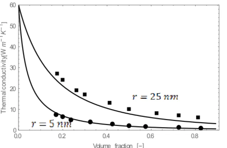
In Fig. 1 is represented the dependence of the effective transversal λ┴ heat conductivity

of wires as a function of the volume fraction for two values of the radius (r=5 and r=25 nm) and s=0 (pure diffusive scattering). Comparison with numerical solutions of the Boltzmann

10

transport equation [19] shows an excellent agreement. For a fixed volume fraction, λ┴

increases with increasing radii. This is easily understood, as in this case the wire-matrix interface decreases and the phonon interface scattering is less important and offers less resistance against heat transport. Otherwise stated, at larger dimensions, the boundary resistance is weaker and the heat conductivities of both the wires and the matrix become close to their respective bulk values characterized by the absence of boundary effects. When the radius of the wire is fixed, one observes generally a lowering of the thermal conductivity with increasing volume fraction due to the increase of the wire-matrix interface.

In Fig.2 are plotted the values of the transversal heat conductivity versus the volume fraction for two values of the radius (5 and 50 nm). The predictions from our model are compared to Fourier’s law. In the latter case, the results are not sensitive to size, as it should, and the values of the heat conductivity are systematically overestimated. The effect of the thermal boundary resistance, measured through the parameter α is displayed in Fig.2 wherein the results of the model are compared with those of a zero Kapitza resistance α=0. One notices that the heat conductivity is larger for α=0 which is understandable as it corresponds to the weakest boundary resistance. Moreover, the larger is the size of the wire, the greater is the difference between a zero and a non-zero α-value, because for larger sizes a change in the value of α will have larger consequences, due to the larger wire-matrix interface. Our results are of the same order of magnitude as those obtained by Behrang et al [14] who limited their analysis to α=0. Moreover, their analysis is not based on extended thermodynamics but follows a different route mixing EMA and Boltzmann’s theory. Fig. 2 shows that the effect of a non-vanishing α becomes important at large volume fractions and wire sizes. However, since in most nanocomposites, the volume fractions of nanoparticles is relatively small, taking α ≠ 0 has little impact in actual applications.

11 0.0 0.2 0.4 0.6 0.8 0 10 20 30 40 50 60 Volume fraction T he rm al co nd uc tiv ity W m 1K 1

Fig. 1. Transversal effective thermal conductivity of Si/Ge nanocomposite as a function of the volume fraction of the nanowires for two values of the radius (r= 5 and 25 nm) and s=0. The results are compared with Boltzmann‘s solutions represented by circles for r= 5 nm and squares for r= 25 nm. 100 4 0.001 0.010 0.100 10 20 30 40 50 60 Volume fraction T he rm al co nd uc tiv ity W m 1 K 1 r_p 50 nm; 0 r_p 5 nm; 0 rp 50 nm; Fourier r_p 5 nm; Fourier rp 50 nm r_p 5 nm

Fig. 2. Transversal effective thermal conductivity versus the volume fraction of nanowires for r= 5, 50 nm. Comparison with Fourier’s law and with zero Kapitza resistance α=0.

In the study of transverse heat conduction, it was admitted that the length of the wires was infinite, in other words much larger than the radii of the wires. To check the validity of

12

this approximation, we have calculated the effective heat conductivity λ┴ for several lengths

of the nanowire at various values of the volume fractions and different sizes. Fig. 3(a)

indicates clearly that for a wire radius of 25 nm, λ┴ remains practically constant whatever the

length of the wire and the volume fraction. It is true that for large radii, the length has little influences on the transversal heat conductivity. Nevertheless, looking more closely to Fig. 3(b) indicates that for a radius comparable or larger than the length, there is a more significant influence, albeit this effect is much smaller than that of the volume fraction or the wire radius. It is also worth to stress that all the figures have been limited to φ=π/√12 which corresponds to the maximum packing of rigid cylindrical nanowires.

0 20 40 60 80 100 0 10 20 30 40 50 60 L nm T he rm al co nd uc tiv ity W m 1K 1 0.5 0.3 0.2 0.1 0.05 0.02 0.01 0 20 40 60 80 100 0 10 20 30 40 50 60 L nm T he rm al co nd uc tiv ity W m 1K 1 r 200 nm r 100 nm r 75 nm r 50 nm r 25 nm r 15 nm r 5 nm

Fig.3. Effect of the longitudinal length L on the transversal heat conductivity for (a) several volume fractions and r= 25 nm and (b) several wire radii and φ=0.1.

In the above analysis, it was assumed that the interface was perfect i.e. characterized by s=0. In order to appreciate the role of the specularity s, we have presented in Fig. 4 the results of the variation of the transversal heat conductivity as a function of the wire length L, for several values of s. The volume fraction is fixed at φ=0.1 and three values of the radius are investigated (r=5, 25 and 100 nm).

13 0 20 40 60 80 100 0 10 20 30 40 50 60 L nm T he rm al co nd uc tiv ity W m 1K 1

Fig.4. Effect of the longitudinal length L on the transversal heat conductivity for several s-values with φ=0.1 and r= 5, 25, 100 nm.

As far as the effect of the s-value on the transversal heat conductivity is concerned, we see from Fig. 4 that the only visible differences occur between s=0 and s=0.1. No significant differences are observed between s=0.1 and s=1. The main reason is that the flow of phonons normal to the surface is not greatly affected by the nature of the surface; this is no longer true with the longitudinal phonons moving along the interface, as shown below.

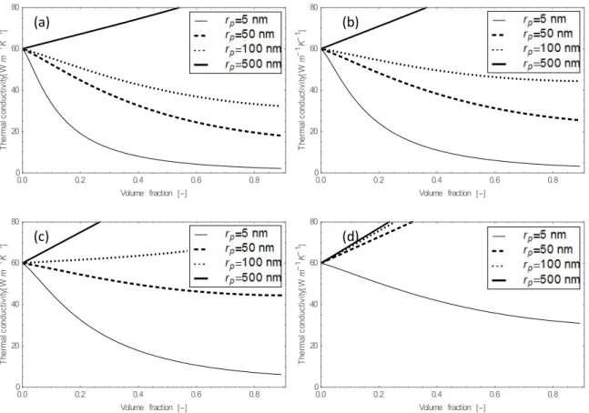
The results corresponding to heating in the longitudinal direction are plotted in Fig. 5 for four values of the specularity parameter (s= 0, 0.2, 0.5 and 0.9). For s= 0, heat conductivity is decreasing with the volume fraction and with decreasing sizes. However, by increasing sufficiently either the radius or the s-value (each independently), the heat conductivity increases with the volume fraction. Increasing the values of s means a reduction of the roughness of the particles-matrix interface whence less obstacles are experienced by the phonons and therefore a higher heat conductivity is predicted. Larger wire radii also mean smaller interfaces between the wires and the matrix, with, as a consequence, less obstacles for the phonons and an increase in the heat conductivity. From a mathematical point of view, a larger wire radius and a higher s-value lead to smaller Knudsen numbers, characteristic of the

14

Fourier regime. The heat conductivity is then simply a combination of the bulk heat conductivities. Since that of the wires (Si) is larger than that of the matrix (Ge), the heat conductivity will increase with larger volume fractions. So, whether the longitudinal heat conductivity increases or decreases as a function of the volume fraction depends on the three factors: wire radius, surface specularity and bulk heat conductivities.

0.0 0.2 0.4 0.6 0.8 0 20 40 60 80 Volume fraction T he rm al co nd uc tiv ity W m 1K 1 0.0 0.2 0.4 0.6 0.8 0 20 40 60 80 Volume fraction T he rm al co nd uc tiv ity W m 1K 1 0.0 0.2 0.4 0.6 0.8 0 20 40 60 80 Volume fraction T he rm al co nd uc tiv ity W m 1K 1 0.0 0.2 0.4 0.6 0.8 0 20 40 60 80 Volume fraction T he rm al co nd uc tiv ity W m 1K 1

Fig. 5. Longitudinal heat conductivity as a function of volume fraction for four values of the radius (r= 5, 50, 100, 500) and various values of s (a) s=0, (b) s=0.2, (c) s=0.5, (d) s=0.9.

4. Temperature dependence of the thermal conductivity

We enlarge the investigations discussed in the previous sections by examining the role of temperature. This is achieved by replacing expression (4) of the heat conductivity by the more general relation wherein the frequency ω and temperature-dependence are made explicit, namely

(a) (b)

15 0 1 ( , ) ( , ) ( , ) 3 D v j cj T vj T lj T dw   

_

   j=m, p. (19)

The determination of (19) requires the knowledge of v( , ), ( , ), _, ( , )

j j j b

c T  v T  l T  for j = m, p

and lm, coll(T) in terms of ω and T. The limit of integration, , is the Debye frequency cutoff:

= 5.14 1013 _s-1 _{for Ge and 9.12 10}13 _s-1 _{for Si. In agreement with earlier works [20-22], we}

assume that the phonon group velocity v is independent of the temperature and the frequency. For the specific heat and the mean free path, we take

4 2 3 exp( / ) 3 2 ² ² [exp( / ) 1]² v B j j B B w k T c v k T k T         , j= m, p (20) 1 ² exp( j) j j B T l T     , j= m, p (21)

wherein Bj and θj are constant quantities obtained by fitting experimental data: Bm =1.655 10

-22 _s²m-1_K-1_{, θ}

m=78.92 K, Bp=5.753 10-23 s² m-1 K-1, θp=199.2 K. In the study of temperature

dependence, we will use the values of the material data of the Debye model. We have

reported in Fig. 6, the dependence of λeff as a function of temperature for two values of the

radius (r = 5 and 50 nm) and different volume fractions, varying from φ =0.01 to 0.5, the wires being oriented normal to the heat flux. The heat conductivity is seen to decrease significantly with the temperature at fixed radius and volume fraction. This behavior can be explained by the fact that the thermal boundary resistance is more important at a lower temperature (lower heat capacities) and therefore contributes to a larger reduction of the heat conductivity. At large volume fraction and small particle size, the heat conductivity is shown to remain almost constant. This is a consequence of the strong particle-matrix interaction that prevails on such conditions. In Fig. 7, the overall thermal conductivities in the longitudinal

16

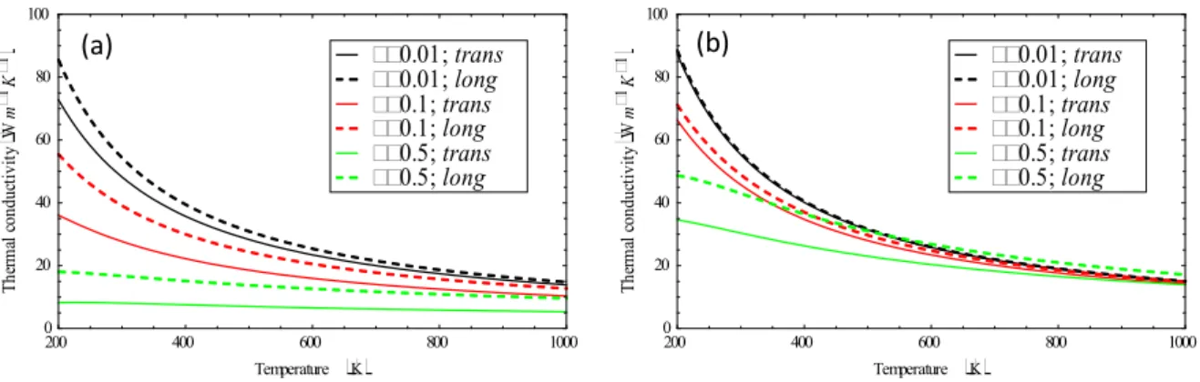
temperature for several values of φ and two different radii. The general behavior is rather similar in the two configurations with the difference that higher values for the thermal conductivity are observed in the longitudinal direction. This is not surprising as phonons experience less boundary scattering while moving in the longitudinal direction.

1000 500 200 300 700 0 20 40 60 80 100 Temperature



K



Th er m al co nd uc tiv it y



W m  1K  1



0.5; r50nm 0.5; r5nm 0.1; r50nm 0.1; r5nm 0.01; r50nm 0.01; r5nm

Fig. 6. Thermal dependence of the transversal effective thermal heat conductivity at several volume fractions and two values of the radius: r= 5, 50 nm.

200 400 600 800 1000 0 20 40 60 80 100 Temperature



K



Th er m al co nd uc tiv ity



W m  1K  1



0.5; long 0.5; trans 0.1; long 0.1; trans 0.01; long 0.01; trans 200 400 600 800 1000 0 20 40 60 80 100 Temperature



K



Th er m al co nd uc tiv ity



W m  1K  1



0.5; long 0.5; trans 0.1; long 0.1; trans 0.01; long 0.01; trans

Fig. 7. Comparison between thermal conductivities in the transversal and longitudinal direction respectively as a function of the temperature for different volumes fractions and for r=5 nm (a) and r=50 nm (b).

5. Conclusions

17

This work is devoted to the study of heat conduction in nanocomposites constituted by dispersed nanowires in a homogeneous matrix. The thermal conductivity depends on several factors as the volume fraction of the nano elements, their size, the nature of the particle-matrix interface and the temperature. Two particular situations have been investigated: nanowires oriented normal and parallel to the heat flow, respectively. The expression of the heat

conductivity λm of the matrix is that of the modified EMA model as proposed by Minnich and

Chen [4], the main originality of the present approach being the derivation of the expression

of the heat conductivity λp of the nanowires. Because their dimensions are comparable to the

mean free path of the energy carrier, the classical Fourier law is no longer valid. Instead, we

propose for λp a relation derived from Extended Irreversible Thermodynamics [5,6,7],

wherein the dependence with respect to the size of the nano wires is made explicit. Special emphasis has been put on the temperature dependence of the heat conductivity, a subject only occasionally treated in the literature. Our results are shown to be in good agreement with those obtained from Boltzmann’s transport equation and other approaches following different routes, which attests of the quality of the present modelling. An advantage is that it rests on simple and explicit mathematical expressions which makes it easily tractable from a computing point of view. The above approach was applied to metalloids wherein the phonons are the only heat carriers. In a future work, it is forecast to generalize it by including metallic materials, wherein the heating is governed by both phonons and electrons.

Acknowledgements

We thank the BelSPo for financial support.

References

18

[2] C. W. Nan, R. Birringer, D. R. Clarke, H. Gleiter, J. Appl. Phys. 81 (1997). [3] A.K.M.M. Morshed, T.C. Paul, J.A. Khan, Physica E 47 (2013) 246.

[4] A. J. Minnich, G. Chen, Appl. Phys. Lett. 91 (2007) 073105.

[5] D. Jou, J. Casas-Vazquez, G. Lebon, Extended Irreversible Thermodynamics, 4rth edition, Springer, New York, Dordrecht, Heidelberg, London, 2010.

[6] G. Lebon, D. Jou, J. Casas-Vazquez, Understanding Non-Equilibrium Thermodynamics, Springer, Berlin, 2008.

[7] G. Lebon, J. Non-Equil. Thermodyn. 39 (2014) 35.

[8] H. Machrafi, G. Lebon, Int. J. Nanosc. 13 (2014) 1450022.

[9] A. Behrang, M. Grmela, C. Dubois, S. Turenne, P.G. Lafeur, J. Appl. Phys. 114 (2013) 014305.

[10] J. Ordonez-Miranda, R. Yang, J.J. Alvarado-Gil, Appl. Phys. Lett. 98 (2011) 233111. [11] J.C. Maxwell, Treatise on Electricity and Magnetism, 2nd edition, Clarendon, Oxford: 1881.

[12] D.P.H. Hasselman, L.F. Johnson, J. Compos. Mat. 21 (1987) 516. [13] G. Chen, Phys. Rev. B 57 (1998) 14973.

[14] A. Behrang, M. Grmela, C. Dubois, S. Turenne, P.G. Lafleur, G. Lebon, App. Phys. Lett . 104 (2014) 063106.

[15] S. Hess, Z. Naturforsch. 32a (1977) 678.

[16] D. Jou, J. Casas-Vazquez, G. Lebon, M. Grmela, Appl. Math. Lett. 18 (2005) 963-967. [17] F. X. Alvarez, D. Jou, Appl. Phys. Lett. 90 (2007) 083109.

[18] G. Chen, Int. J. Therm. Sci. 39 (2000) 471-480.

[19] R. Yang, G. Chen, M.S. Dresselhaus, Phys. Rev. B 72 (2005) 125418.

[20] A. Behrang, M. Grmela, C. Dubois, S. Turenne, P.G. Lafleur, Roy. Soc. Chem. Advances 5 (2015) 2768.

19

[21] N. Mingo, L. Yang, D. Li, A. Majumdar, Nano Lett. 3 (2003) 1713-1716.

[22] G. Chen, Nanoscale Energy Transport and Conversion: A Parallel Treatment of Electrons, Molecules, Phonons, and Photons, Oxford University Press, Oxford, 2005.