HAL Id: hal-00135012
https://hal.archives-ouvertes.fr/hal-00135012v2
Preprint submitted on 2 May 2007
HAL is a multi-disciplinary open access
archive for the deposit and dissemination of sci-entific research documents, whether they are pub-lished or not. The documents may come from teaching and research institutions in France or abroad, or from public or private research centers.
L’archive ouverte pluridisciplinaire HAL, est destinée au dépôt et à la diffusion de documents scientifiques de niveau recherche, publiés ou non, émanant des établissements d’enseignement et de recherche français ou étrangers, des laboratoires publics ou privés.
A Batch Optimization Solver for diffusion area
scheduling in semiconductor manufacturing
Claude Yugma, Christian Artigues, Stéphane Dauzère-Pérès, Alexandre
Derreumaux, Olivier Sibille
To cite this version:
Claude Yugma, Christian Artigues, Stéphane Dauzère-Pérès, Alexandre Derreumaux, Olivier Sibille. A Batch Optimization Solver for diffusion area scheduling in semiconductor manufacturing. 2007. �hal-00135012v2�
A Batch Optimization Solver for diffusion area scheduling in
semiconductor manufacturing
Claude Yugma1 ∗ Christian Artigues2 St´ephane Dauz`ere P´er`es1 Alexandre Derreumaux1 Olivier Sibille3
1Ecole des Mines de Saint-Etienne, Centre Microlectronique de Provence - Site Georges´ Charpak, Avenue des An´emones, Quartier Saint-Pierre, F-13541 Gardanne, France
2LAAS-CNRS, 7 avenue du Colonel Roche, 31077 Toulouse, France 3ATMEL, Zone industrielle, 13790 Rousset, France
Abstract
This paper presents a method and a software for solving a batching and scheduling problem in the diffusion area of a semiconductor plant, the ATMEL fabrication unit in Rousset, France. The diffusion area is one of the most complex area in the fab. A significant number of lots has to be processed while satisfying complex equipment process and line management constraints. The purpose of this study is to investigate approaches to group lots in batches, to assign the batches on the equipment and to sequence these batches. Three indicators are used to evaluate the quality of a solution: the total number of moves, the batching coefficient and the X-factor. The problem is modeled through the disjunctive graph formulation. A constructive algorithm is proposed and improvement procedures based on iterative sampling and simulated annealing are developed. Computational experiments, carried out on actual industrial problem instances, show the ability of iterative sampling to improve significantly the initial solution. The proposed simulated annealing method brings in turn important enhancements to the results of iterative sampling. The software based on these methods, named Batch Optimization Solver (BOS), is currently used in the diffusion area of ATMEL. The disjunctive graph model allows in addition a high level of interactivity with the decision makers.
keyword: Batch scheduling, disjunctive graph, local search, simulated annealing, wafer fabri-cation.
1
Introduction
Semiconductor wafer fabrication can be described as a multistage process with re-entrant flows. The processing is done layer by layer. Each layer requires several steps of processing such as chemical-mechanical polishing, diffusion, film deposition, photolithography, implant (doping) and etching. For each of the product types, and depending on the technology, a wafer goes through more than 400 process steps over a period of a few weeks. Wafer fabrication planning and scheduling is a complex task due to the large number of products and machines involved. It is further complicated by additional constraints such as re-entrant flow of operations [Kum94], setup issues, preventive maintenances, random machine breakdowns, etc.
The importance of scheduling on the performance of semiconductor wafer fabrication facilities is known for many years [Wei88, VS06]. Recently [TIHC05] have also shown the importance of using predictive scheduling in load balancing methods among multiple semiconductor wafer fabrication lines in order to make a better estimation of the lot cycle times. The cycle time is the total time necessary to manufacture a lot of wafers. It measures the duration time spent since the lot enters the fab and the moment it leaves it. According to experimental studies, decreasing the cycle time results in an increase of the productivity in a fab [JH90].
The complexity of the fabrication process is such that most previous existing work on schedul-ing in semiconductor manufacturschedul-ing focus on dispatchschedul-ing rules [Wei88, DF03, VS06]. Other approaches deal with Integer Linear Programming formulations of the problem and apply la-grangean relaxation of the equipment limitation constraints [LCPC96, HC03]. For a given set of lagrangean multipliers, the relaxation can be solved with minimal cost network flow meth-ods. Subgradient optimization is used to solve the dual linear program. A feasible solution is obtained by adjusting heuristically the solution of the relaxation.
In this paper, instead of scheduling the entire fab, we propose to focus on a bottleneck part of the manufacturing process. Among the complex operations involved in the fabrication of a wafer, the diffusion phase is of critical importance since the batching decisions that are involved may affect the performance of the entire wafer fab [ICN+03, MH03]. This is also the case in the ATMEL fabrication unit of Rousset (France). The diffusion phase is used primarily to alter the type and level of conductivity of semiconductor materials. It is used to form bases, emitters and resistors in bipolar devices, and also to dope polysilicon layers. The Batch Optimization Software (BOS) project aims at developing a method and a software for solving efficiently the batching and scheduling problem of the diffusion area while taking into account numerous constraints and optimizing various criteria. Another objective of the BOS is to provide an easy way to build, modify and use the results of the software. As for the global problem, batching and scheduling in diffusion areas is mainly performed in the literature by dispatching rules. In [ICS+03] and [MH03], the authors propose to use a dispatching rule to batch the operations and a genetic algorithm to assign the batches to equipment. In [MFC02], a scheduling problem in semiconductor manufacturing related to the one tackled in this paper is solved by a modified shifting bottleneck heuristic [ABZ88].
In this paper, we propose to model solutions of the considered batching and scheduling prob-lem through a variant of the disjunctive graph proposed in [MFC02]. A constructive heuristic is designed that builds an initial solution as well as improvement procedures based on local search and simulated annealing.
This paper is organized as follows. In Section 2, we give the problem description. In Section 3, we present the proposed disjunctive graph representation. The method for computing an initial solution and improvement procedures based on iterative sampling and simulated annealing are described in Section 4. Experimental results are given on real problem instances issued from the Rousset ATMEL fabrication unit in Section 5. The BOS software is briefly presented in Section 6. The Section 7 concludes the paper with recommendations for further research.
2
Problem description
The diffusion area defines a batching and scheduling problem of wafer lots on two types of equipment: furnaces and cleaning machines. These resources are able to perform several lots simultaneously. Each lot requires one or more consecutive operations on the equipments and each operation has a recipe which determines its duration and the set of machines that are able to process it. On a 24-hour basis, each operation has to be assigned to an equipment, and included into a batch, i.e. a set of operations of the same recipe that are processed simultaneously by the
equipment. The constraints in the diffusion area are divided into 3 types: equipment constraints, process constraints and line management constraints.
2.1 Constraints
Some of these constraints are common to the two types of resources while others are dedicated to furnaces.
2.1.1 Equipment constraints • Common constraints
Dedicated equipment: any equipment is able to process a limited set of recipes.
Maximum batch size: any equipment defines a maximum batch size corresponding to the capacity of that equipment.
Loading and unloading times: a time may be needed to load and unload a batch on the equipment.
Unavailability periods: the equipment may be unavailable during some periods (defined by time windows) due to qualification, repair, maintenance etc.
In process jobs: the equipment may be occupied at the beginning of the time horizon by in-process operations that have to be completed before the equipment becomes available. • Specific furnace constraints
Minimum time between two batches on an furnace: some furnaces must be inspected at the end of each processed batch.
2.1.2 Process constraints • Common constraints
Precedence: lot operations must be performed following the manufacturing process of the lot. The operations of a lot are chained and no operation can start before the end of its predecessor, except for the first operation of each lot.
Minimum time lag: there is a fixed handling and transport time between every two suc-cessive operations of a lot.
Release dates: they correspond to the arrival times of lots at the cleaning machines and furnaces. It means that a lot cannot be scheduled before its release date. Because the diffusion area is a stage of the complex global production process, the release date are precomputed by a simulation package designed by ATMEL.
Fixed recipe: each operation of a lot is associated with a recipe, i.e. the lot should be processed on resources that are qualified for the corresponding recipe. This implies that all lots in the same batch must be processed with the same recipe.
Process time: the process time of a batch on an equipment depends on the recipe. Maximum time lag: a time limit is given for two successive operations x and y of a lot. The difference between the starting time of y and the completion time of x cannot exceed this limit. Maximum time lags depend on the operations x and y. They can correspond to the maximum time limit between cleaning and furnace equipment.
2.1.3 Line management constraints
• Specific furnace constraints Minimum distance between two batches of same recipe: there is a minimum time between the beginning of two batches of the same recipe on two different furnaces.
2.2 Objectives
In semiconductor factories, several indicators are used to measure the performance of a fab. We describe thereafter the indicators that are relevant in our study. The interested reader can refer to [MT06] for more details.
• The number of moves (to maximize): It corresponds to the number of completed opera-tions on the planning horizon, which can be compared to the target number fixed by the production managers.
• Batching coefficient (to maximize): Defined on the planning horizon, it is calculated as the number of moves divided by the sum of the number of batches performed on each machine, times the maximum capacity of that machine. Note that the denominator is the number of lots that could be performed if the equipment was loaded up to their maximum capacities.
• The X-factor (to minimize): This indicator is used to evaluate the waiting times of lots in the diffusion area in order to reduce the cycle times. For a given lot, this factor is calculated as the total staying time of the lot in the diffusion area (i.e. waiting time from its arrival in the diffusion area and processing time) over its processing time.
These three indicators will be used to evaluate solutions in the fab.
Others indicators not considered in this paper are of interest. Among them, the Work-In-Process (WIP), is defined as the number of wafers being in the fab at a given period, either in a production state or in a non-production state (e.g. transport and waiting). The law of Little [Lit61] establishes that if a system is stable and stationary then the average WIP is proportional to the average cycle time. The throughput is defined as the outgoing number of wafers of the fab per unit of time. The evolution of the throughput in time makes it possible to know if the system is stable i.e. to know if there is no accumulation of product in the fab or if the system evolves/moves according to forecasts. Authors, such as [GR88], observed that there is a relation between the increasing of the throughput and the output of a fab. The cycle time drastically increases when throughput is close to the maximal capacity of the fab. Hence for both WIP and throughput indicators, the X-factor indicator is adequate.
The goal is to optimize the various performance measures, while taking into account the numerous complex constraints. Another objective is to make the proposed schedule easily mod-ifiable by the decision makers at the fabrication level. Machines may be declared as down, operations may be moved, lots may be removed or inserted. Such requirements can be achieved thanks to the flexibility of the disjunctive graph representation.
The next subsection described the mathematical formulation used to model the problem.
2.3 Problem Formulation
The scheduling problem can be formulated as follows. For sake of clarity, the above-described Unavailability periods, In-process jobs and Minimum distance between batches of the same recipe constraints are not included. In Section 3, we describe how we tackle these additional charac-teristics.
A set of jobs (lots) J = {Ji|i = 1, . . . , n} has to be processed during a period T by a set
of machines M = {Mk|k = 1, . . . , m}. Each job Ji is made of ni operations such that each
operation Oij has a duration pij > 0 and a set Mij ⊆ M of machines (the furnaces or the
cleaning equipments of the diffusion area) able to process it. Let Ok = {Oij ∈ O|Mk ∈ Mij}
elements of the set Mij are determined by the recipe of operation Oij denoted ρij. In general
we have Mij ⊂ M since each machine cannot be configured for all recipes. Each operation
Oij has to be included in a batch on a resource k ∈ Mij. Each machine has a finite capacity
Rk which gives the maximal number of lots in the same batch. On each machine k, Sk denote
the setup time needed before starting a new batch, Dk denote the removal time needed after
the completion of a batch and sk denote the constant setup time needed between two different
batches. s0
k denotes the initial setup time on machine k, depending on the state of the resource
at time 0. Two consecutive operations Oij and Oi(j+1)of the same job are linked by minimal and
maximal time lags. Once the batch of Oij is completed and removed from k, the setup for the
batch of Oi(j+1) cannot start before a minimal time lag τmin
ij and has to start before a maximal
time lag τijmax. Let O = {Oij|i = 1, . . . , n; j = 1, . . . , ni} denote the set of all operations. Each
job Ji has a relative priority ci (ci < cj =⇒ Ji is more urgent than Jj). Each job corresponds
to a number wi of wafers produced when the job is completed. Finding a feasible solution for
the problem lies in making four types of decisions: D1 - Partition the operations into batches, D2 - Select a resource to process each batch, D3 - Order the batches on each resource, D4 - And assign a start time to each batch.
Decisions D1-D3 can all be represented by a family of batches B = {Bkq}k∈{1,...,m},q∈{1,...,νk} where Bkq is the batch sequenced at position q on machine Mk. νk ∈ {0, . . . , |Ok|} denote
the number of batches assigned to machine Mk. Decision D4 lead to a family of start times
T = {tij}Oij∈O assigned to the operations. Once a solution {B, T } is determined, we can deduce a machine assignment {mij}Oij∈O where mij denote the machine Oij is assigned to, i.e. verifying ∃q ∈ {1, . . . , νk} such that Oij ∈ Bmijq. To be feasible, a solution {B, T } and its corresponding assignment {mij}Oij∈O have to satisfy the following constraints. The operations of the same batch must have the same recipe, i.e.
ρij = ρxy ∀B ∈ B, ∀Oij, Oxy ∈ B (1)
Each operation must be assigned to a machine able to process its recipe.
mij ∈ Mij ∀Oij ∈ O (2)
The batch capacity cannot be exceeded and each batch includes at least one operation.
1 ≤ |Bkq| ≤ Rk ∀Bqk∈ B (3)
An operation appears in only one batch i.e.
B ∩ B′= ∅ B, B′ ∈ B, B 6= B′ (4)
All operations are included in a batch
∪B∈BB = O (5)
The start time of the first operation of each lot cannot exceed the lot release date:
Each operation Oij, j > 1, cannot start before a minimal time lag after the end of preceding
operation Oi(j−1), which takes account of the removal time of the batch of Oi(j−1), the minimal
time lag τi(j−1)min and the setup time of batch of Oij:
tij − ti(j−1) ≥ Dmi(j−1)+ pi(j−1)+ τi(j−1)min + Smij
∀i ∈ {1, . . . , n}, ∀j ∈ {2, . . . , ni} (7)
Each operation Oij, j > 1, has to start before a maximal time lag after the end of preceding
operation Oi(j−1), which takes account of the removal time of the batch of Oi(j−1), the maximal
time lag τi(j−1)max and the setup time of batch of Oij:
tij − ti(j−1) ≤ Dmi(j−1)+ pi(j−1)+ τi(j−1)max + Smij
∀i ∈ {1, . . . , n}, ∀j ∈ {2, . . . , ni} (8)
The start times of two operations of the same batch must be equal:
tij = txy ∀B ∈ B, ∀Oij, Oxy ∈ B (9)
An operation of a batch which is not at the first position on its machine cannot start before the end of the preceding batch on the machine, plus the necessary removal time of the preceding batch, plus the minimal setup time on the machine between two batches, plus the necessary setup time for the next batch.
tij− txy ≥ pxy+ Dk+ sk+ Sk
∀Bkq,q>1 ∈ B, ∀Oij ∈ Bkq, ∀Oxy ∈ Bk(q−1) (10)
An operation of a batch in the first position on its machine cannot start before the initial setup time for this batch (we assume Sk0≤ Sk+ Dk+ sk, ∀Mk∈ M):
tij ≥ s0mij ∀Oij ∈ O (11)
By definition, a feasible solution includes each operation inside a batch. In the ATMEL Rousset production unit, the scheduling horizon is in fact limited to a scheduling period T . Hence only those batches released in the interval [0, T [ must be taken into account. Several criteria are used to measure the quality of a feasible solution. The number of moves is the number of wafers produced during the time period T:
fmov = X
Ji∈J
wiθi (12)
where θi= 1 when the job is completed before T and θi ∈ [0, 1[ denotes the completion ratio of
job i before time T otherwise.
θi = P Oij,tij+pij<=T pij + P Oij,tij<T <tij+pij (T − tij) Pni j=1pij
The batching coefficient is the average ratio of the actual size of each batch over to its maximal size. Let BT = {B ∈ B|t
ij < T, ∀Oij ∈ B} denote the set of batches started before
time period T . batching coefficient = P k P Bkq∈BT|Bkq|/Rk |BT| (13)
fbatch = P k P Bkq∈BT |Bkq|/(Rk+ Zk 100) |BT| (14)
where Zk means the number of total qualified recipe on the machine k.
The weighting of the coefficient of batching by the number of qualified recipes on the concerned machine makes it possible to use the least general-purpose machines initially.
The average X-factor is the average of the X-factor of each job weighted by the job priority. All the jobs do not have the same priority. Certain jobs are more important than others (im-portant customers, tests to be carried out quickly, delay to catch up with, etc). Thus, a weight is affected to the job to reflect the priority. Let JT = {J
i ∈ J |tini+ pini ≤ T } denote the set of jobs completed before T .
X-fac = P Ji∈JT(tini− ri)/pini |JT| (15) fX-fac = P Ji∈JTci(tini− ri) |JT| (16)
The choice made together with the decision makers in the ATMEL Rousset unit is to combine these different objectives into a single one by minimizing the weighted sum
f = αfmov + βfbatch − γfX-fac (17)
where α, β and γ are adjustable weights allocated to each objective function. The objective functions have been designed to integrate some requests of ATMEL managers. On the one hand, in the calculation of fX−f ac, the delay of each lot is multiplied by its priority, in order to support
the urgent lots. On the second hand, in the calculation of the total batching coefficient, the batching coefficient of each equipment is multiplied according to the number of qualified recipes on this equipment. This leads to occupy in priority the equipments able to treat less recipes, and thus to maintain the availability of the most flexible equipments.
The objective of the problem is to search for a feasible selection {B, T } such that f is maximized. Note that given a (feasible) solution {B, T }, f can be computed in O(N ) time where N = Pn
i=1ni is the total number of operations.
3
The disjunctive graph representation
The considered problem can be seen as an extension of the job-shop problem and, consequently, the disjunctive graph model can be used for batching and scheduling problems as proposed by [MFC02]. In their article, the authors consider a different objective function (namely total weighted tardiness). Sequence-dependant setup times and reentrant flows are also tackled but there are no maximum time lags. Unfortunaly, these latter constraints increase considerably the difficulty of the problem [GNST04]. Let us explain how we modeled the problem using disjunctive graphs.
We define the disjunctive graph G = (V, C, E) as follows.
• V is a set of nodes where there is one node per operation, denoted Vij, plus a dummy start
node denoted 0.
• C is the set of conjunctive arcs representing the release dates and minimal and maximal time lags. There is an arc from node 0 to node Vi1 of each job Ji. There is an arc from Vij
to Vi(j+1) and an arc from Vi(j+1) to Vij, for each consecutive operations Oij and Oi(j+1)
• E is the set of disjunctive arcs which represent the decisions of the problem. There are two opposite disjunctive arcs (Vij, Vxv)k and (Vxy, Vij)k for any machine k ∈ M and for
any pair of operations Oij, Oxy ∈ Ok, Oij 6= Oxy. These arcs represent the sequencing or
the batching decision concerning Oij and Oxy on machine k.
Let B denote a partial or complete batching for the problem satisfying at least constraints (1), (2), (3) and (4). B is a complete batching if constraint (5) is also verified, otherwise it is a partial batching . Recall B also defines the machine assignment mij, for all Oij ∈ ∪B∈BB. We
assume mij = 0 if Oij is not batched in B, i.e. if we have Oij 6∈ ∪B∈BB.
B unambiguously defines a selection S as follows. For each distinct operations Oij and Oxy
such that mij = mxy = k 6= 0, select arc (Vxy, Vij)k if Oxy is in a batch sequenced before the
batch of Oij, select arc (Vij, Vxy)k if Oij is in a batch sequenced before the batch of Oxy, and
select both arcs (Vij, Vxv)k and (Vxy, Vij)k if Oij and Oxy are assigned to the same batch.
Once a selection is computed, we define a graph G(S) = (V, C ∪ S) where arcs C ∪ S are valuated as follows (we assume s0
0 = s0= S0= D0 = 0):
• Each arc from 0 to the first operation Oi1 is valuated by max(ri, Sm0ij), the maximal value between the release date of job i and the initial setup time for machine mi1.
• Each arc from Vij and Vi(j+1) is valuated by Dmij+ pij+ τ
min
ij + Smi(j+1), the value of the minimal time lag between Oij and Oi(j+1) plus the setup and removal times linked to the
assignment of the operations.
• Each arc from Oi(j+1)and Oij is valuated by −(Dmij+pij+τ
max
ij +Smi(j+1)), the (negative) value of the maximal time lag between Oij and Oi(j+1)plus the necessary setup and removal
times.
• Each arc (Vij, Vxv)k is valuated either by pij + Dk+ sk+ Sk if the opposite arc is not
selected or by 0 if the opposite arc is selected. Indeed, in the first case this arc represent the decision to sequence Oxy after Oij on machine k whereas in the second case, both arcs
(Vij, Vxv)k and (Vxv, Vij)k represent the sychronisation of the operations included in the
same batch.
We can state that the (partial) solution represented by the (partial) batching B and its selection S is feasible if and only if all longest path problems from node 0 to each node Vij in
G(S) have a solution. In the positive case and if B is complete, a feasible schedule T can be obtained by setting tij to the length of the longest path from 0 to Vij. Furthermore T is the
best schedule compatible with B one can obtain when the objective is to maximize f .
The problem can be formulated as follows: Find the batching B verifying constraints (1), (2), (3), (4) and (5) such that the corresponding selection S is feasible and maximizes f .
As stated in the previous sections, the actual data issued from the fab has other character-istics that have been tackled, such as in-process jobs and machine down times. We can model easily these characteristics thanks to the disjunctive graph formulation. They can be both rep-resented by operations with fixed start times on the involved machine. A start time t can be fixed by linking the node with node 0 by two opposite arcs valued by t and −t. As stated in Sec-tion 2, the actual problem also includes an important line management constraint: a minimum distance between the start time of two batches of the same recipe scheduled on two different batches has to be respected. This can also be tackled through the disjunctive graph represen-tation. A fictitious machine can be associated to each recipe and disjunctive arcs linking two operations of the same recipe can be defined. Then, whenever the two operations are batched on two different machines (furnaces), the disjunctive arc has to be orientated. Once orientated the arc is valuated by the minimum required distance.
4
Solution Methods
We propose a two-phase heuristic method to solve the problem. The first phase is a constructive heuristic based on successive job insertions. The second phase is a local search method which aims at improving the initial solution. Both phases are based on the evaluation of a (complete or partial) selection through longest path calculations.
4.1 Evaluation of a partial or complete batching
Any partial or complete batching B and its selection S can be evaluated through the calculation of start time tij, equal to the longest path from 0 to Vij in G(S) of each operation Oij. To
compute such longest paths, since the graph includes arcs with negative weights, we use the Bellman-Ford algorithm which has a O(N |S ∪ C|) time complexity. If the algorithms finds a path of positive length, then the partial or complete solution is unfeasible. Otherwise the algorithm returns start times tij and the objective function value f can be determined.
4.2 Computing an initial solution by a priority rule-based constructive heuris-tic
The initial solution (selection) is computed by a simple job insertion method. The jobs are first sorted in a list L according to the order: jobs involving maximal time lags first, then increasing release dates, then job priority.
The method starts with an empty batching. Then the jobs are taken in the order given by the list and inserted one by one in the current batching. The insertion of Ji is made as follows.
Let B = {Bkq}k∈M,q∈1,...,νk denote the current batching including jobs located before Ji in L. For each operation Oij of Ji and for each resource k ∈ Mij, there are 2νk+ 1 insertion positions
of Oij in the batch sequence of machine Mk: indeed, for each batch Bkq, we may insert Oij
inside batch Bkq or create a new batch at any position. Each of these insertion positions is
evaluated with the algorithm described in the previous section and the one that maximizes f is kept to update B. If none of the insertion positions is feasible for an operation Oij then all these
partial solutions violate a maximal time lag and there exists insertion positions that violate only maximal time lag between Oi(j−1) and Oij (the last position on each resource of Mij, for
instance). Hence we have to remove Oi(j−1) from B, the previous operation of job Ji, and insert
it at a later insertion position. If this is not feasible, they are not scheduled and delayed from the list of operations. Note that at mostPni
j=1
P
k∈Mij2νk+ 1 insertion positions are tested per inserted lot.
4.3 Improving the initial solution by iterative sampling
Iterative random sampling consists in applying iteratively the constructive algorithm presented in Section 4.2 changing each time the input operation list randomly. Two different iterative sampling methods are proposed. The random sampling method initialize defines the input list of each iteration as a random permutation. The pseudo-random sampling method computes the list by making slight random modifications on the sorted list. It consists in dividing the list into intervals and, for each interval, in making a random modification following a uniform law.
4.4 Simulated annealing
Simulated annealing (SA) belongs to the class of randomized local search algorithms and has been developed by [KGV83] to handle hard combinatorial problems. The use of simulated
annealing supposes the definition of a combinatorial optimization problem and a neighborhood. We are here looking for a solution to the considered batching and a scheduling problem with the maximal objective function value. The neighborhood we consider is defined by the following moves:
1. ”Batch move”. A batch is moved randomly (both equipment and position can change). 2. ”Operation move”. An operation is moved randomly in an existing batch or a new batch
is created (both equipment and position can change).
3. ”Operation switch” Two batches with the same recipe are selected randomly. Then two randomly selected operations are switched.
50% of the considered moves are batch moves, 25% are operation moves and 25% are oper-ation switches. According to the move, randomly generated, we proceed as follows. All random selections are made according to the uniform law. If a move is impossible due to a violation of a constraint, we restore the current solution, we try another move and we reiterate. Each neighbor solution is evaluated y means of the longest path computations presented in Section 4.1. The algorithm starts with an initial solution s0 and then continually tries to find better solutions by searching in its neighborhood (obtained by the moves described above), and applying a stochastic acceptance criterion. When a neighbor (a solution s) of the current solution is selected we compare the difference ∆f = f (s) − f (s0). If the difference ∆f is negative, the neighbor replaces the current solution. Otherwise, if the difference is positive the neighbor is accepted with a probability based upon the Boltzmann distribution Paccept(∆f ) ≈ exp(−∆fkT )
where k is a constant and the temperature T is a control parameter. This temperature is gradually lowered following a geometrical law function g(T ) : g(T ) = αT with α < 1.
5
Computational experiments
We have coded the proposed algorithms in Java and we have tested them on a 1 gigaoctet RAM and 3.4 gigahertz processor computer. These tests have been performed on 8 actual instances of the problem issued for 8 production days in the ATMEL Rousset factory. There are 700 jobs yielding a total number of 1400 operations with about 50 different recipes to schedule on about 70 furnaces, and each of them has a capacity between 4 and 6 lots. There are 12 cleaning equipment with capacity about 2 to 4 lots. The time needed to load and unload a batch varies between 10 and 30 minutes. The minimum and maximum time lags varie from 10 minutes to 4 hours. The target time horizon is 24 hours. The weights of the components of the objective function have been computed both to normalize the different indicators and to take account of the user preferences. For the experiments, we have selected α = 601, β = 1500001, γ = 41.
In Table 1, we display the objective function value (experssion 17), the number of moves expression 12), the batching coefficient (expression 13), the X-factor (expression 15) and the required computational time of the 8 solutions obtained by the constructive method.
From Table 2 to Table 5, we display the results of 1000 runs of the random sampling method, the pseudo-random sampling method and the simulated annealing heuristic for the 4 indicators (objective function, number of moves, batching coefficient, X-factor) separately.
The percentage correspond for each instance to the relative improvement brought by 1000 runs of the considered method over the reference solution obtained by the constructive heuristic, i.e. Best solution−Sorted listSorted list . We also display the standard deviation over the 1000 runs for each method and each instance.
The computational times are 1000 times greater than the constructive heuristic for the random sampling and pseudo-random sampling methods. The computational time of each run of the simulated annealing algorithm has been limited to 360 seconds.
The analysis of the Table 1 shows that we get the initial solution in a rather fast computation time: the smallest time is 9 seconds and the the largest time is 17 seconds. For the managers of the diffusion area, obtaining a solution in a fast time was a key issue. We underline also that the constructive method provides solutions which are evaluated as satisfactory by the ATMEL managers. They also point out that the results are consistant with the operator practices. This was also an important point for the ATMEL managers who would not accept that the proposed initial solutions change too deeply the organization of the diffusion area. Consequently the first results we obtained were well accepted in the fab and constituted good start points for further improvement.
Let us consider the results of the random and pseudo-random sampling method for the objective function (Table 2). The improvements brought by the random sampling method are better than the ones brought the pseudo random sampling method. The analysis of standard deviation allows us to state that the random list covers a greater solution space, meaning that there is a capability of reaching better solutions, but also worse. Indeed, we obtain an objective function increase of 6, 77% in the best case and of 0, 00% in the worst case for random sampling while for pseudo random sampling, the increase is of 6, 52% in the best case and of 0, 85% in the worst case. Among all instances, the average improvements are of 3,66% for random sampling and 3% for pseudo random sampling. Globally the random and pseudo-random sampling method succeed in improving the objective function at the expense of larger compuational times.
Looking separately at the objective function components, the move indicator, the batching coefficient, the X-factor are slightly improved in average showing the relative quality of the initial solution. The weighting of the delay by the priority of the batches makes it possible to schedule the most urgent batches first. Similarly, the weighting of the batching coefficient by the number of qualified recipes on the concerned equipment makes it possible to fill the least general-purpose machines first. For some instances (060317 for the random method and 060428 for the pseudo-random method), we can notice that the objective function is improved while the indicators are worsened which is a consequence of the selected weights.
For simulated annealing, the initial solution is taken according to the best solution obtained by the random sampling method and the pseudo random sampling method. First, it must be reported that there is no significant difference between starting from a high temperature or a low temperature. The displayed results correspond to a temperature equal to 32000 and the step parameter is set to 25. Considering we start from an initial solution which was already improved by (pseudo-)random sampling, the fact of starting from a high temperature does not have a significant influence on the objective function. Globally, the objective function can be improved up to 12,36 % (starting from the best random sampling solution) and 12,37% (starting from the best pseudo random sampling solution). The average objective function improvement is of 8,31% (random) and of 7,05% (pseudo random).
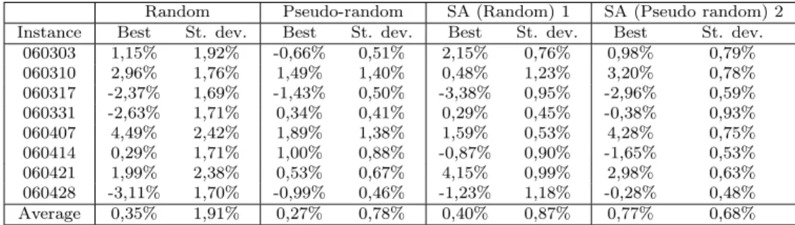
The “number of moves” indicator is rather difficult to improve. The majority of the tests slightly worsen it but we can reach an improvement on it up to 4,15% (random) and 4,28% (pseudo random). The average improvement for move indicator is of 0,40% (random ) and 0,77% (pseudo random) (see Table 3). The batching coefficient can be improved up to 3,78% (random list) and 4,04% (pseudo random list). For this indicator the average improvements are 1,24% (random list) and 2,16% (pseudo random list) (see Table 4). The X-factor is the indicator where the improvements are the most significant. There are improvements which go up to 5,22% (random) and 6,52% (pseudo random). The average improvement is of 2,81% (random) and 3,37% (pseudo random) (see Table 5). In comparison to the results of random
and pseudo-random sampling, we improve in average a lot more each indicator. Again, at the expense of extra computational times, the simulated anealing algorithm succeeds in improving significantly the results of the sampling methods.
6
The BOS software
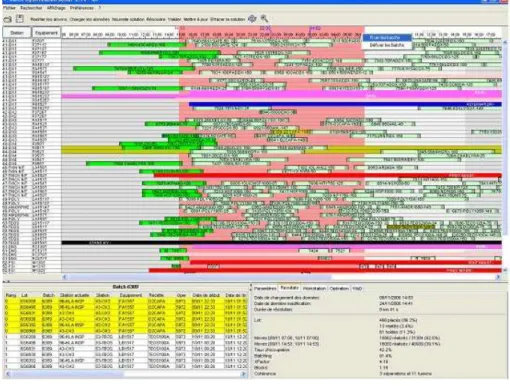
The use of a disjunctive graph brings significant improvements for interactive scheduling at the fab level. A prototype software (Figure 1 gives the graphical user interface of the software), the Batch Optimization Software, has been developed jointly by ATMEL, the University of Avignon (LIA) and the ´Ecole des Mines de Saint-Etienne (CMP Gardanne). It includes the off-line batching and scheduling phase, as described above, and also an interactive module that allows the decision-makers to make modifications and to test options directly on the proposed plan. The longest path calculations in the disjunctive graph allow to almost immediately give the impact of a modification such as job removal, operation move, job or operation insertion. The software is currently in phase of intensive test in the ATMEL diffusion area.
7
Concluding remarks
We have proposed a model and a method based on a disjunctive graph for batching and schedul-ing problem in a semiconductor manufacturschedul-ing factory while takschedul-ing into account complex con-straints and optimizing multiple measures. A constructive algorithm has been proposed to solve the problem, local search improvements based on the disjunctive graph representation have been defined and a simulated annealing algorithm has been developed. The computational tests made on real instances of ATMEL showed that we obtain quality solutions in fast calculation times. The simulated annealing procedure improve significantly the different criteria (number of moves, batching coefficient and X-factor) in comparison with a simple local search method.
This research can be extended in many ways. Other types of moves such as the simultaneous move of 2 jobs linked by a maximum time lag should be tested. The maximal time lags are currently hard constraints. However in practice some of them can be relaxed and treated as soft constraints or objectives. Another important issue can be in a multicriteria analysis study. Computing several Pareto solutions are useful particularly when the situation frequently changes as it is usually the case of semiconductor factories.
Acknowledgements
This work is part of the MEDEA+ European project HYMNE (High Yield driven MaNufacturing Excellence in sub 65 nm CMOS), partly funded by the “Minist`ere de l’´Economie, des Finances et de l’Industrie” (French Ministry of Economy, Finance and Industry).
References
[ABZ88] J. Adams, E. Balas, and D. Zawack. The shifting bottleneck procedure for job shop scheduling. Management Science, 34:391–401, 1988.
[DF03] R. M. Dabbas and J. W. Fowler. A new scheduling approach using combined dis-patching criteria in wafer fabs. IEEE Transactions on Semiconductor Manufacturing, 16(3):501–510, 2003.
[GNST04] K. Gentner, K. Neumann, C. Schwindt, and N. Trautmann. Batch production scheduling in the process industries. In J.Y.T. Leung, editor, Handbook of Schedul-ing: Algorithms, Models and Performance Analysis, pages 48.1–48.21. CRC Press, Boca Raton, 2004.
[GR88] C. Glassey and M. Resende. Closed-loop job release control for vlsi circuit manufac-turing. IEEE Transactions on Semiconductor manufacturing, 1(1):36–46, 1988. [HC03] T.-K. Hwang and S.-C.g Chang. Design of a lagrangian relaxation-based
hierarchi-cal production scheduling environment for semiconductor wafer fabrication. IEEE Transactions on Robotics and Automation, 19(4):566–578, 2003.
[ICN+03] K. Ibrahim, M. A. Chik, W. S. Nizam, N. L. Fem, and N. F. Za’bah. Efficient lot batching system for furnace operation. In IEEE/SEMI Advanced Semiconductor Manufacturing Conference, pages 322–324, 2003.
[ICS+03] K. Ibrahim, M. A. Chik, W. S.Nizam, N. L. Fem, and N. F. Za’bah. Efficient lot batching system for furnace operation. In IEEE/SEMI Advanced Semiconductor Manufacturing Conference, pages 322–324, 2003.
[JH90] G.S. JR and T. Hout. Competing against time: how time-based competition is reshapping global markets. Technical report, The Free Press, 1990.
[KGV83] S. Kirkpatrick, C. Gelatt, and M. Vecchi. Optimization by simulated annealing. Science, tome 220(4598):671–680, 1983.
[Kum94] P.R. Kumar. Scheduling semiconductor manufacturing plants. IEEE Control Systems Magazine, 14(6):30–40, 1994.
[LCPC96] D.-Y. Liao, S.-C. Chang, K.-W. Pei, and C.-M. Chang. Daily scheduling for r&d semiconductor fabrication. IEEE Transactions on Semiconductor Manufacturing, 9(4):550–560, 1996.
[Lit61] J. Little. A proof for the queuing formula l = λw. Operations Research, 9:383–387, 1961.
[MFC02] S.J. Mason, J.W. Fowler, and W.M. Carlyle. A modified shifting bottleneck heuristic for minimizing total weighted tardiness in complex job shops. Journal of Scheduling, 5(3):247–262, 2002.
[MH03] L. Monch and I. Habenicht. Simulation-based assessment of batching heuristics in semiconductor manufacturing. In S. Chick, P.J. Sanchez, D. Ferrin, and D. J. Morrice, editors, Winter Simulation Conference, pages 1338–1345. ACM, 2003.
[MT06] J. Montoya-Torres. Manufacturing performance evaluation in wafer semiconduc-tor facsemiconduc-tories. International Journal of Productivity and Performance management, 55(3/4):300–310, 2006.
[TIHC05] H. Toba, H. Izumi, H. Hatada, and T. Chikushima. Dynamic load balancing among multiple fabrication lines through estimation of minimum inter-operation time. IEEE Transactions on Semiconductor Manufacturing, 18(1):202–213, 2005.
[VS06] A. Varadarajan and S. C. Sarin. A survey of dispatching rules for operational control in wafer fabrication. In A. Dolgui, G. Morel, and C. E. Pereira, editors, 12th IFAC Symposium on Information Control Problems in Manufacturing, pages 715–726, 2006.
[Wei88] L. M. Wein. Scheduling semiconductor wafer fabrication. IEEE Transactions on Semiconductor Manufacturing, 1(3):115–130, 1988.
Figure 1: Interface of the prototype
Instance Objective Moves Batching X-factor Time
060303 -6,13E+07 15115 0,73 3,13 12 s 060310 -4,16E+07 15193 0,79 2,98 13 s 060317 -5,88E+07 16383 0,75 3,29 17 s 060331 -4,50E+07 14804 0,75 2,45 11 s 060407 -5,02E+07 13112 0,70 3,39 9 s 060414 -3,53E+07 13912 0,76 2,91 9 s 060421 -5,57E+07 13845 0,69 2,95 11 s 060428 -4,86E+07 15748 0,70 3,53 13 s
Random Pseudo-random SA (Random) 1 SA (Pseudo-random) 2 Instance Best St. dev. Best St. dev. Best St. dev. Best St. dev.
060303 0,00% 1,59% 6,52% 0,47% 8,32% 1,22% 12,37% 0,82% 060310 2,64% 1,78% 1,20% 0,90% 11,32% 1,34% 8,57% 1,18% 060317 1,53% 1,31% 0,85% 0,41% 9,96% 1,08% 4,69% 0,64% 060331 1,56% 1,38% 1,56% 0,44% 4,12% 0,48% 4,36% 0,58% 060407 6,77% 2,17% 6,18% 1,57% 3,45% 0,70% 7,40% 1,00% 060414 5,38% 2,40% 5,10% 2,10% 6,08% 1,00% 6,23% 0,96% 060421 5,21% 1,88% 0,90% 0,30% 12,36% 0,85% 5,72% 0,70% 060428 6,17% 1,66% 1,65% 0,54% 10,91% 0,83% 7,05% 0,81% Average 3,66% 1,77% 3,00% 0,84% 8,31% 0,94% 7,05% 0,84%
Table 2: Results of the improvement methods (Objective function)
Random Pseudo-random SA (Random) 1 SA (Pseudo random) 2 Instance Best St. dev. Best St. dev. Best St. dev. Best St. dev.
060303 1,15% 1,92% -0,66% 0,51% 2,15% 0,76% 0,98% 0,79% 060310 2,96% 1,76% 1,49% 1,40% 0,48% 1,23% 3,20% 0,78% 060317 -2,37% 1,69% -1,43% 0,50% -3,38% 0,95% -2,96% 0,59% 060331 -2,63% 1,71% 0,34% 0,41% 0,29% 0,45% -0,38% 0,93% 060407 4,49% 2,42% 1,89% 1,38% 1,59% 0,53% 4,28% 0,75% 060414 0,29% 1,71% 1,00% 0,88% -0,87% 0,90% -1,65% 0,53% 060421 1,99% 2,38% 0,53% 0,67% 4,15% 0,99% 2,98% 0,63% 060428 -3,11% 1,70% -0,99% 0,46% -1,23% 1,18% -0,28% 0,48% Average 0,35% 1,91% 0,27% 0,78% 0,40% 0,87% 0,77% 0,68%
Table 3: Results of the improvement methods (Number of moves)
Random Pseudo-random SA (Random) 1 SA (Pseudo random) 2 Instance Best St. dev. Best St. dev. Best St. dev. Best St. dev.
060303 2,73% 1,26% 1,36% 0,35% 3,67% 0,73% 2,98% 0,64% 060310 -3,80% 1,06% -2,53% 0,61% -1,68% 0,66% 0,70% 0,51% 060317 0,00% 1,19% -1,33% 0,47% 0,16% 0,94% 0,59% 0,56% 060331 -1,33% 1,16% -1,33% 0,55% 1,71% 0,37% 2,36% 0,50% 060407 1,43% 1,32% 1,43% 0,57% 3,78% 0,67% 4,04% 0,53% 060414 -1,32% 1,29% 0,00% 0,75% -0,80% 0,50% 2,88% 0,71% 060421 1,45% 1,28% 1,45% 0,31% 1,02% 0,68% 2,03% 0,50% 060428 1,43% 1,16% 0,00% 0,51% 2,02% 0,35% 1,72% 0,60% Average 0,07% 1,22% -0,12% 0,52% 1,24% 0,61% 2,16% 0,57%
Table 4: Results of the improvement methods (Batching coefficient)
Random Pseudo-random SA(Random) 1 SA(Pseudo random) 2 Instance Best St. dev. Best St. dev. Best St. dev. Best St. dev.
060303 0,95% 1,62% 0,95% 0,52% 0,86% 0,99% 5,22% 0,16% 060310 2,35% 1,53% 0,00% 1,56% 4,48% 1,12% 3,58% 0,14% 060317 -1,22% 1,32% 0,61% 0,56% 1,23% 0,80% 1,24% 0,13% 060331 0,82% 1,82% 2,45% 0,95% 2,00% 1,03% 4,40% 0,16% 060407 -1,77% 1,42% -0,29% 0,54% 5,00% 0,90% 6,52% 0,12% 060414 -0,34% 1,44% 1,03% 0,86% 4,24% 1,08% 3,08% 0,20% 060421 -3,73% 1,75% -1,69% 0,35% 1,50% 1,25% 0,10% 0,12% 060428 0,28% 1,12% 0,00% 0,28% 3,18% 0,93% 2,82% 0,12% Average -0,33% 1,50% 0,38% 0,70% 2,81% 1,01% 3,37% 0,14%