Global Identification of Joint Drive Gains and Dynamic Parameters of Robots

(1)

HAL Id: hal-00979950

https://hal.archives-ouvertes.fr/hal-00979950

Submitted on 25 Jun 2019

HAL is a multi-disciplinary open access

archive for the deposit and dissemination of sci-entific research documents, whether they are pub-lished or not. The documents may come from teaching and research institutions in France or abroad, or from public or private research centers.

L’archive ouverte pluridisciplinaire HAL, est destinée au dépôt et à la diffusion de documents scientifiques de niveau recherche, publiés ou non, émanant des établissements d’enseignement et de recherche français ou étrangers, des laboratoires publics ou privés.

Global Identification of Joint Drive Gains and Dynamic

Parameters of Robots

Maxime Gautier, Sébastien Briot

To cite this version:

Maxime Gautier, Sébastien Briot. Global Identification of Joint Drive Gains and Dynamic Parameters of Robots. Journal of Dynamic Systems, Measurement, and Control, American Society of Mechanical Engineers, 2014, 136 (5). �hal-00979950�

(2)

M. Gautier, S. Briot 1 Paper DS-13-1373

Global Identification of Joint Drive Gains and Dynamic Parameters

of Robots

Maxime Gautier1,2_{and Sébastien Briot}1,*

1_{Institut de Recherches en Communications et Cybernétique} de Nantes (IRCCyN), UMR CNRS 6597, Nantes, France

1 rue de la Noë, BP 92101, F-44321 Nantes Cedex 03 FRANCE Maxime.Gautier@irccyn.ec-nantes.fr Sebastien.Briot@irccyn.ec-nantes.fr 2_{University of Nantes}

2 Chemin de la Houssinière, 44300 Nantes FRANCE

*

Corresponding author

Phone: + 33 (0)2 40 37 69 58 Fax: + 33 (0)2 40 37 69 30

(3)

Abstract

Off-line robot dynamic identification methods are based on the use of the Inverse Dynamic Identification Model (IDIM), which calculates the joint forces/torques that are linear in relation to the dynamic parameters, and on the use of linear least squares technique to calculate the parameters (IDIM-LS technique). The joint forces/torques are calculated as the product of the known control signal (the input reference of the motor current loop) by the joint drive gains. Then it is essential to get accurate values of joint drive gains to get accurate estimation of the motor torques and accurate identification of dynamic parameters. The previous works proposed to identify the gain of one joint at a time using data of each joint separately. This is a sequential procedure which accumulates errors from step to step. To overcome this drawback, this paper proposes a global identification of the drive gains of all joints and the dynamic parameters of all links. They are calculated altogether in a single step using all the data of all joints at the same time. The method is based on the total least squares solution of an over-determined linear system obtained with the inverse dynamic model calculated with available input reference of the motor current loop and joint position sampled data while the robot is tracking some reference trajectories without load on the robot and some trajectories with a known payload fixed on the robot. The method is experimentally validated on an industrial Stäubli TX-40 robot.

Keywords: Industrial robots, Drive gains, Dynamic parameters identification

I. INTRODUCTION

(4)

M. Gautier, S. Briot 3 Paper DS-13-1373 robots [1]–[8]. Most of the dynamic off-line identification methods:

- use an Inverse Dynamic Identification Model (IDIM) that gives the linear relations between the joint forces/torques and the dynamic parameters,

- build an over-determined linear system of equations obtained by sampling the IDIM while the robot is tracking some trajectories in position closed-loop control,

- estimate the parameter values using least squares techniques (LS). This procedure is called the

IDIM-LS technique.

Good experimental results can be obtained if:

- a well-tuned derivative band-pass filtering of joint position is used to calculate the joint velocities and accelerations,

- accurate values for joint drive gains are known to calculate the joint force/torque as the product of the input references of the motor current loop by the joint drive gains [9], [10].

This requires the calibration of the drive train constituted by a current controlled voltage source amplifier with gain G which supplies a permanent magnet DC or a brushless motor with torque _t

constant K coupled to the link through direct drive or gear train with gear ratio N . Because of _t

large values of the gear ratio for industrial robots, (N>50), the total joint drive gain, g_ NG K_t _t,

is very sensitive to errors in G and _i K which must be accurately measured from special, time _t

consuming, heavy tests on amplifiers and motors, which require opening the drive chain of each joint [9], [10]. This sensitivity to errors directly affects the accuracy of the force/torque computation as well as the interaction force between the robot and its environment or payload estimations that are required in many modern robotic applications.

More recent works [11], [12] have proposed to apply sequential procedures to identify the total joint drive gains g__j for each actuated joint separately by using a known payload fixed on the

(5)

end-effector. In both methods, the estimation of the drive gain of one joint was done using only data coming from the corresponding joint equation which implies the loss of information about the coupled data on the other joints. With these sequential approaches, leading to error accumulation, good results were obtained only for the first four robot joints.

In this paper, a new method is proposed for the global identification of all robot dynamic parameters, including joint drive gains, using the input reference of the motor current loop and the joint position sampled data while the robot is tracking one reference trajectory without

load fixed on the robot and one trajectory with a known payload fixed on the robot. Inertial

payload parameters are measured or calculated with a CAD software. Contrary to the previous works, all dynamic parameters and drive gains are calculated in one step as the Total LS solution

(TLS) of an over-determined system that takes into account the coupling between the robot axes.

Such a method avoids the cumulative errors of the previous sequential procedures. In order to show the method efficiency, it is experimentally validated on an industrial robot manufactured by Stäubli: the TX-40.

It should be mentioned that this method is easy to implement, versatile and suitable for the automatic calibration of the drive gains of any industrial robots.

A first condensed version of this work has been proposed in [13]. The present paper contains detailed explanations on the TLS procedure to enlighten the theoretical understanding of the

method, especially in terms of statistical properties, and gives additional experimental results that show the interest of the method in terms of force/torque estimation and parameter identification.

(6)

M. Gautier, S. Briot 5 Paper DS-13-1373 II. USUAL IDENTIFICATION PROCEDURE WITH INVERSE DYNAMIC MODEL AND LEAST SQUARES

(IDIM-LS)

A. Inverse Dynamic Identification Model (IDIM)

It is known that, using the modified Denavit-Hartenberg description of moving multibody systems [6], the dynamic model of any serial manipulator composed of n links and n actuators

can be linearly written in term of a



n_st vector of standard parameters 1



χ [5], [6]: _st

( , ) ( )

idm , ,  st  st , ,  st

τ q q q χ IDM q q q χ (1)

where τ_idm is the motor torque vector, q , q and q are respectively the



n_{ vectors of}1



generalized joint positions, velocities and accelerations, IDM is the _st



n n _st



Jacobian matrix of τ_idm with respect to (w.r.t.) the vector χ of the standard parameters given by _st

1 2 _...

T T T n T

st   st st st 

χ χ χ χ .

For a rigid robot, the link j and joint j can be parameterized by 14 standard parameters regrouped into the vector j

st χ such that j T j st  XX XY XZ YY YZ ZZ MX MY MZ M Ia Fv Fsj j j j j j j j j j j j joff  χ , where:

 XX_j, , , , , XY XZ YY YZ ZZ are the six components of the inertia matrix _j _j _j _j _j I of link j w.r.t. _j

frame j at its origin, i.e.

j j j j j j j j j j XX XY XZ XY YY YZ XZ YZ ZZ            I

 M is the mass of link j , _j Ia is a total inertia moment for rotor of actuator j and gears of the _j

(7)

M. Gautier, S. Briot 6 Paper DS-13-1373  MX_j, , MY MZ are the 3 components of the first moment of link j , i.e. _j _j

T j j j j j j j M O S_{ }MX MY MZ _ where j j j

O S is the position of the center of mass of the link j expressed in the frame attached at the origin of the considered link [6]

 Fv , _j Fs are the viscous and Coulomb friction coefficients of the drive chain, respectively, _j

and

j

off

 is an offset parameter which regroups the amplifier offset and the asymmetrical Coulomb friction coefficient [14].

The identifiable parameters are the base parameters, which are the minimal number of dynamic parameters from which the dynamic model can be calculated. They are obtained from the standard parameters by eliminating those which have no effect in (1) and by regrouping some of the others by means of linear relations [15], using simple closed-form rules [6], [16], or by numerical method based on the QR decomposition [17].

The minimal dynamic model can be written using the n base dynamic parameters denoted as _b

χ as follows:

( )

idm  , , 

τ IDM q q q χ (2)

where IDM is a subset of independent columns of IDM which defines the identifiable _st

parameters.

Because of perturbations due to noise measurement and modeling errors, the actual force/torque τ differs from τ_idm by an error, e , such that:

(8)

( )

idm , ,

     

τ τ e IDM q q q χ e (3)

where τ is calculated with the drive chain relations:

1 ₀ 1 0 n n v g v g                _{ } _{  }               τ v g (4) 

v is the (n n matrix of the actual motor current references of the current amplifiers () _vj



corresponds to actuator j) and g is the (_ n vector of the joint drive gains (1)

j j

j

j t t

g_ N G K

corresponds to actuator j, where

j

t

G is the gain of the current controlled voltage source amplifier

of the motor j which supplies a permanent magnet DC or a brushless motor with torque constant

j

t

K coupled to the link through direct drive or gear train with gear ratio N ) that is given by a _j

priori manufacturer’s data or measured with special time-consuming heavy tests on amplifiers

and motors separately [9], [10].

Equation (3) represents the Inverse Dynamic Identification Model (IDIM).

B. IDIM with a payload

The payload is considered as a link n_{ fixed to the link n of the robot [18]. Only}1 n among its _kL

ten inertial parameters are considered to be known (i.e. there is n_uL 10n_kL unknown

parameters). The model (3) becomes:



uL kL



uL tot tot kL      _ _       χ

τ IDM IDM IDM χ e IDM χ e χ

(5)

(9)

M. Gautier, S. Briot 8 Paper DS-13-1373 parameters of the payload; IDM is the (_aL n n _aL) Jacobian matrix of τ_idm, w.r.t. the vector χ . _aL

C. Least Squares Identification of the Dynamic Parameters with IDIM

The off-line identification of the robot base dynamic parameters χ can be achieved given

measured or estimated off-line data for τ and



q q q , collected while the robot is tracking , , 



some trajectories. The model (3) is sampled, low-pass filtered and decimated (parallel decimation of Y and each column of W ) in order to get an over-determined linear system of (n r ) equations and nb unknowns:

 

_



_ˆ _{ }ˆ ˆ



_

Y τ W q,q,q χ ρ (6)

where ( )q, q, q is an estimation of ( )ˆ  ˆ ˆ q, q, q , obtained by sampling, band-pass filtering the  

measure of q with zero-phase non causal butterworth filter and central difference algorithm [5], ρ

is the (r vector of errors, and 1) W q, q, q is the (



ˆ  ˆ ˆ



r n _b) observation matrix.

In [2], [19], practical rules for tuning these filters and for avoiding a biased estimation of the velocities and accelerations [20] are given, taking advantage of non-causal off-line pass-band filtering.

Using the base parameters and tracking “exciting” reference trajectories, i.e. optimized trajectories that can be computed by nonlinear minimization of a criterion function of the condition number of the W matrix [21], [22] a well-conditioned matrix W can be obtained. In this work, the motion generator of the industrial controller which is a point-to-point trapezoidal acceleration generator is used. Some trajectories are tested covering the whole robot workspace

(10)

until a good criterion is obtained [22], which is an easy and fast procedure that gives good identification results. The LS solution ˆχ of (6) is given by:









ˆ _ T 1 T _ 

χ W W W Y W Y (7)

It is computed using the QR factorization of W . Standard deviations _ˆ

i





, are estimated assuming that W is a deterministic matrix and , is a zero-mean additive independent Gaussian noise, with a covariance matrix C , such that [2]: _

T 2

( ) _r

E

  

C ρρ I (8)

E is the expectation operator and Ir, the (r r identity matrix. An unbiased estimation of the )

standard deviation



_ is: 2

2 ₍ ₎

b

ˆ_ ˆ r n

  Y Wχ  (9)

The covariance matrix of the estimation error is given by [2]:

T 2 T 1 [( )( ) ] ( ) ˆ ˆ E ˆ ˆ ˆ       C χ χ χ χ W W (10) 2 _{( )} i ˆ ˆ ˆ i,i  

  C is the ith diagonal coefficient of C __{ˆ ˆ}

The relative standard deviation

ri ˆ %_ is given by: 100 ri i ˆ ˆ ˆi %_  _  (11) for ˆ_i  . 0

The ordinary LS can be improved by a weighted LS procedure (IDIM-WLS) where data in Y and W are sorted w.r.t. each joint j equation and weighted with the inverse of the standard deviation of the error calculated from ordinary LS solution of the equations of joint j [19].

(11)

D. Identification with a payload

In order to identify both the robot and the payload dynamic parameters, it is necessary that the robot carried out two types of trajectories: (a) trajectories without the payload and (b) trajectories with the payload fixed to the end-effector [18]. The sampling and filtering of the IDIM (5) is then written as: a a uL b b uL kL kL      _{  } _{  } _{  }    _{  }   χ Y W 0 0 Y χ ρ Y W W W χ (12)

where Y (_a Y , resp.) is the vector of sampled input torques of the robot in the unloaded (loaded, _b

resp.) case, W (_a W , resp.) is the observation matrix of the robot in the unloaded (loaded, resp.) _b

case and W (_uL W , resp.) is the observation matrix of the robot corresponding to the unknown _kL

(known, resp.) payload inertial parameters.

III. GLOBAL IDENTIFICATION OF THE ROBOT DYNAMIC PARAMETERS AND THE DRIVE GAINS

A. Least Square Identification of the Robot Dynamic Parameters and the Joint Drive Gains

In the usual IDIM-WLS, accurate values of the drive gains are necessary to compute vector Y. However, the manufacturer’s data give drive gains parameters g with an uncertainty of about _

10%, thus leading to parameter identification and torque estimation errors. Therefore, it is preferable to introduce the drive gains into the base parameters.

(12)

M. Gautier, S. Briot 11 Paper DS-13-1373 1 a a uL b b uL kL kL         _{  } _ _ _ _{  }    _{  }   χ V W 0 0 Y g χ ρ V W W W χ (13)

where V (__a V , resp.) is the block-diagonal matrix of __b v samples in the unloaded (loaded, resp.) _

case, 1 ,1 , n , , j j a b j r v v               _ _ _ _               V 0 V V 0 V , (14) , j k

v_ is the k-th sample of current reference for actuator j, and j



V regroups all the current

reference samples for actuator j.

A simple approach to identify the drive gains is to take into account that the vector W χ is _{kL kL}

known. Then (13) can be rewritten as:

a a L r r kL kL b b uL uL          _{  }         _ _ _{  }    _{  }   g 0 V W 0 Y χ ρ W χ ρ W χ V W W χ (15)

with χ the vector of the unknown inertial parameters of the robot and the payload plus the drive _r

gain parameters.

As a result, the LS solution ˆχ of (15) is given by: _r







1



ˆ T T r r r r kL kL r L  _   χ W W W W χ W Y (16)

Because Y and _L W depend on the same data containing perturbations _r ( )q, q, q (due to the ˆ  ˆ ˆ use of W in _kL Y and of _L W in _uL W ), the noises in _r Y and _L W are correlated which may _r

introduce a bias. This is shown in our case study (Table VII).

(13)

M. Gautier, S. Briot 12 Paper DS-13-1373 Total Least Squares Identification (IDIM-TLS) procedure. This procedure is detailed below.

B. Total Least Square Identification of the Robot Dynamic Parameters and the Joint Drive Gains (IDIM-TLS)

Details on the TLS identification method can be found in [23], [24] and many other papers (see also [25]–[27]). Eq. (13) can be rewritten as:

tot tot  W χ ρ , (17) where a a tot b b uL kL kL        _ _ _    V W 0 0 W

V W W W χ is a (r c matrix (with ) c n n n  b+ uL ), and 1

1

T T T T

tot    uL 

χ g χ χ is a



c vector. 1



Without perturbation, ρ 0 and  W must be rank deficient to get the non-null solutions _tot

ˆ ˆn

tot  tot 

χ χ 0 (where ˆn tot

χ is a vector of unit norm, i.e. ˆn 1 tot 

χ ) depending on a scale

coefficient . However because of the measurement perturbations, W is a full rank matrix. _tot

Therefore, the system (17) is changed to the compatible system closest to (17) w.r.t. the Frobenius norm:

ˆ ˆ_{tot tot} 

W χ 0 , ˆT ˆT ˆT ˆT 1 tot    uL 

χ g χ χ (18)

where ˆW is the _tot (r c rank deficient matrix, closest to ) W w.r.t. the Frobenius norm, i.e. _tot

ˆ tot

W minimizes the Frobenius norm _tot ˆ_tot

F 

W W and ˆT ˆT ˆT ˆT 1 tot    uL 

χ g χ χ is the solution

of the compatible system (18) closest to (17). ˆ

tot

W can be computed thanks to the “economy size” Singular Value Decomposition (SVD) of

tot

(14)

M. Gautier, S. Briot 13 Paper DS-13-1373 T

tot 

W U S V , (19)

where U and V are (r r and () c c orthonormal matrices, respectively, and ) Sdiag s( )_i is a

(c c diagonal matrix with singular values ) s of _i W sorted in decreasing order. ˆ_tot W is given _tot

by:

ˆ T

tot  totsc c c

W W U V , (20)

where s is the smallest singular value of _c W and _tot U (_c V , resp.) the last columns of U (V, _c

resp.) corresponding to s . Then, the normalized optimal solution ˆ_c n tot

χ is given by the last column

Vc of V, ˆχntot V , which belongs to the kernel of ˆc W . tot

There is infinity of vectors ˆ ˆn tot  tot

χ χ which are solutions of (18) depending on a scale factor

. The unique solution _ˆ* ˆ_ˆn tot  tot

χ χ for the robot can be found by taking into account that the last

value _ˆ*

c

tot

 of _ˆ* tot

χ must be equal to 1 according to (18), i.e. ˆ 1/ ˆ

c n tot   , with ˆ c n tot

 the last value of ˆn

tot

χ .

It must be mentioned that the TLS method has been applied in [29] for the identification of the drive gains and the dynamic parameters on a two degrees of freedom (dof) robot but gave arguable results due to the lack of accurate reference parameters (in [29], the reference parameter was the drive gain of actuator 1 that was not accurately known). As a result, the authors were not able to correctly identify payload masses added on the end-effector. In this paper, a major

improvement is to scale the parameters using the accurate weighed value of an additional payload mass.

(15)

C. Statistical analysis

Standard deviations _ˆ

i



 on the dynamic and drive gains parameters, are estimated assuming that all errors in data matrix W are independently and identically distributed with zero mean and _tot

common covariance matrix C_WW such that

2 ˆ W WW W r C I , (21) where W r

I is the identity matrix of dimension (r c   . ) (r c)

An unbiased estimation of the standard deviation ˆ_W is [24]: ˆ_W s_c/ r c

   (22)

The covariance matrix of the estimation error is approximated by [24]:







1: 1 1: 1



1 2 2 ˆ ˆ ˆ 1 ˆ_{1: 1 2} ˆ c ˆ c T W c tot tot         C χ W W (23)

with χˆ_{1: 1}_c_ the vector containing the c first coefficients of 1 _ˆ* tot χ and 1: 1 ˆ c tot  W a matrix composed

of the c first columns of ˆ1 W . Finally, _tot 2

ˆi Cˆ ˆ( , )i i

 

  is the ith diagonal coefficient of C __{ˆ ˆ}

and the relative standard deviation % _ˆ

ri   is given by: % _ˆ 100 _ˆ ˆ ri i i       , for ˆ_i ≠ 0. In order to improve the estimation of _ˆ*

tot

χ , the rows of W are weighted taking into account _tot

the confidence on the measures. As proposed in IDIM-WLS (Section II.B), to improve the TLS solution, each row corresponding to joint j equation is weighted by the inverse of ˆj

W

 , i.e. the standard deviation corresponding to the data of the joint j equations.

(16)

M. Gautier, S. Briot 15 Paper DS-13-1373 IV. CASE STUDY

A. The Stäubli TX-40 Robot

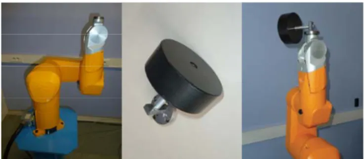
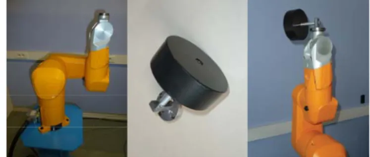
The Stäubli TX-40 robot (Fig. 1) has a serial structure with six rotational joints. Details on its kinematics can be found in [13]. It is to be noted that the payload is numbered as the link 7, rigidly fixed on the last robot joint numbered as the link 6.

Fig. 1. TX-40 robot and its calibrated payload of 4.59 Kg.

The TX-40 robot is characterized by a coupling between the joints 5 and 6 such that:

5 5 5 6 6 6 6 45 0 32 32 qr N q qr N N q            _ _              , 5 5 6 6 5 6 6 0 c r c r N N N       _ _     _ _            (24)

where qr_j is the velocity of the rotor of motor j, q_j is the velocity of joint j, Nj is the transmission gain ratio of axis j, τcj is the motor torque of joint j, taking into account the coupling effect on the motor side, τrj is the electro-magnetic torque of motor j.

The model for the coupled geared drive chain of joints 5 and 6 adds 3 supplementary inertia, viscous and Coulomb friction parameters Ia , _m₆ Fv and _m₆ Fs to both τ_m₆ c5 and τc6:

(17)

M. Gautier, S. Briot 16 Paper DS-13-1373 6 5 6 5 6 6 6 6 6 6 6 5 6 6 5 5 5 6 ( ), + ( ) m m m m c m c m Ia q q q q Ia q q q q Fv Fs sign Fv Fs sign                      (25)

where τj already contains the terms of the uncoupled joints ( ( ) )

j

j j j j j j off

Ia q  Fv q Fc sign q  . The TX-40 IDIM is automatically computed using the software Symoro+ [30] which applies a

recursive and optimized Newton-Euler algorithm that gives the model expression with the minimal number of operations [6].

B. Identification Results

To validate the proposed method, a calibrated payload is used (Fig. 1). Its mass has been measured with an accurate weighing machine (M7 = 4.59 kg ± 0.005 kg). The other parameters

have been calculated using CAD software. Their values are set in bold font in Table I.

Before presenting the identification result, it is to be noticed that during the identification process, some small base parameters remain poorly identifiable because they have no significant contribution in the joint torques [18]. These essential parameters, which are a subset of the base parameters, can be cancelled in order to simplify the dynamic model. They are calculated using an iterative procedure starting from the base parameters estimation. At each step the base parameter which has the largest relative standard deviation is cancelled. A new TLS parameter

estimation of the simplified model is carried out with new relative error standard deviation

ˆ %

ri 

 . The procedure ends when max(% _ˆ ) / min(% _ˆ )

ri ri r

  

   , where r_ is a ratio ideally chosen between 10 and 30 depending on the level of perturbation in Y and W.

The robot joint drive gains and dynamic parameters are identified using four different methods:  Case 1: with the IDIM-WLS method introduced in Section III.A, taking advantage of the

(18)

M. Gautier, S. Briot 17 Paper DS-13-1373 knowledge of the ten payload parameters, to calculate the vector Y of (15), _L

 Case 2: similar to Case 1, but considering the knowledge of the payload mass only,

 Case 3: with the IDIM-TLS method introduced in Section III.B, taking advantage of the knowledge of the ten payload parameters,

 Case 4: similar to Case 3, but considering the knowledge of the payload mass only.

The obtained results are shown in Tables I to IV. The parameters with the subscript R stand for

the regrouped parameters [6]. The results show in all cases that the error on the identified drive gains grows up to 30%! In the case where the payload mass is used only, some identified payload parameters are far from the a priori CAD values. These results could be explained by the fact

that parameters extracted from CAD data are not accurate due to differences between CAD and reality (errors on material properties, payload shape, etc.). It can also be noticed in Tables I and III that the relative difference between the identified parameters is generally small with a mean value less than 10%.

(19)

M. Gautier, S. Briot 18 Paper DS-13-1373 TABLEI

THE ESSENTIAL DYNAMIC PARAMETERS OF THE TX-40IDENTIFIED WITH IDIM-WLS.

with 10 cad param. with 1 weighed mass m7

parameter id.val. % _ˆ ri    id.val. % _ˆ ri   %ei ZZ1R 1,17e+0 2,28 1,14e+0 2,66 2,56 Fv1 6,35e+0 2,37 6,21e+0 2,70 2,20 Fs1 5,18e+0 3,80 4,98e+0 4,10 3,86 XX2R -4,54e-1 3,53 -4,43e-1 3,81 2,42 XZ2R -1,43e-1 5,85 -1,43e-1 5,88 0,00 ZZ2R 9,85e-1 1,36 9,60e-1 1,92 2,54 MX2R 1,97e+0 1,57 1,92e+0 2,21 2,54 Fv2 4,17e+0 2,09 4,09e+0 2,52 1,92 Fs2 7,28e+0 2,60 7,09e+0 2,91 2,61 XX3R 9,56e-2 13,42 9,14e-2 13,84 4,39 ZZ3R 1,19e-1 5,50 1,16e-1 5,75 2,52 MX3 3,63e-2 24,39 3,77e-2 23,00 3,86 MY3R -5,19e-1 2,69 -5,02e-1 3,30 3,28 Ia3 7,52e-2 7,29 7,39e-2 7,44 1,73 Fv3 1,46e+0 3,22 1,42e+0 3,60 2,74 Fs3 5,81e+0 2,87 5,64e+0 3,29 2,93 XY4 - - -5,27e-3 35,04 - MX4 -1,53e-2 18,62 -1,34e-2 21,25 12,42 Ia4 2,50e-2 4,63 2,36e-2 5,55 5,60 Fv4 6,54e-1 2,49 6,37e-1 3,76 2,60 Fs4 1,72e+0 3,11 1,68e+0 4,26 2,33 MY5R -2,40e-2 14,60 -2,26e-2 15,67 5,83 Ia5 4,69e-2 8,11 4,24e-2 9,28 9,59 Fv5 1,24e+0 3,63 1,21e+0 4,56 2,42 Fs5 2,81e+0 3,87 2,71e+0 4,83 3,56 Ia6 9,80e-3 6,29 8,33e-3 7,77 15,00 Iam6 8,49e-3 19,92 8,95e-3 18,72 5,42 Fv6 4,57e-1 2,07 4,34e-1 3,51 5,03 Fvm6 4,30e-1 3,21 4,11e-1 4,31 4,42 Fsm6 1,52e+0 2,95 1,53e+0 4,11 0,66 off6 - - 7,91e-2 24,72 - XX7 0.64e-1 - 8,39e-2 5,79 31,09 XY7 -1.80e-2 - -1,19e-2 17,55 33,89 XZ7 2.60e-2 - 2,22e-2 9,69 14,62 YY7 0.64e-1 - 8,20e-2 5,82 28,13 YZ7 2.60e-2 - 3,18e-2 5,33 22,31 ZZ7 4.40e-2 - 5,21e-2 3,92 18,41 MX7 -2.90e-1 - -2,43e-1 3,29 16,21 MY7 -2.90e-1 - -2,54e-1 3,41 12,41 MZ7 4.10e-1 - 3,91e-1 3,90 4,63 M7=4.59±0.005 M7=4.59±0.005 -

rel. err. norm ||ρ||/||Y|| =12.40% rel. err. norm ||ρ||/||Y||=12.43%

, ˆ

(% ) : 7.86%,_i _{a b}

mean e Y V g  _,

1 2 1

ˆ ˆ ˆ

%e_i  _i _i / _i %., where ˆ1_i is the i-th parameter of IDIM-WLS using the knowledge of the ten payload parameters and ˆ_i2 is the i-th parameter of IDIM-WLS using the knowledge of the payload mass only.

(20)

M. Gautier, S. Briot 19 Paper DS-13-1373 TABLEII

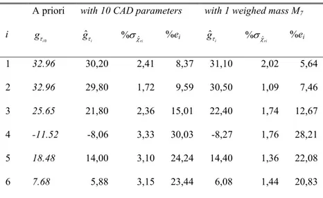
THE DRIVE GAINS OF THE TX-40:APRIORI STAÜBLI’S DATA AND IDENTIFIED VALUES WITH

IDIM-WLS.

A priori with 10 CAD parameters with 1 weighed mass M7

i 0 i g_ ˆ i g_ % _ˆ ri   %ei ˆ i g_ % _ˆ ri   %ei 1 32.96 30,20 2,41 8,37 31,10 2,02 5,64 2 32.96 29,80 1,72 9,59 30,50 1,09 7,46 3 25.65 21,80 2,36 15,01 22,40 1,74 12,67 4 -11.52 -8,06 3,33 30,03 -8,27 1,76 28,21 5 18.48 14,00 3,10 24,24 14,40 1,36 22,08 6 7.68 5,88 3,15 23,44 6,08 1,44 20,83 (% ) :18.45%_i mean e mean(% ) :16..5%e_i ˆ % ri 

 : relative standard deviation.

0 0 ˆ % / % i i i i e  g g g . C. Cross-Validations

To validate the methods used in Cases 1 to 4, obtained results are cross-validated. Three trajectories, different from each other and from the one used for identification (condition number of the corresponding observation matrices is given in Table V), are performed with the robot on which is fixed the payload of 4.59 kg. The positions and current measured are recorded during the robot displacements. Then, the observation matrix is computed for each trajectory.

First, the actuator torques calculated with the relation (4) τ v g (where  _{ }ˆ v is the measured _

(21)

torques computed using the IDIM (2) τ IDMχ ( ˆχ are the identified dynamic parameters). Five  ˆ sets of parameters are chosen:

1. drive gains given by the manufacturer and robot and payload dynamic parameters identified using a classical IDIM-WLS procedure [18],

2. drive gains and robot/payload dynamic parameters identified with the IDIM-WLS method

introduced in Section III.A, with the knowledge of the ten payload parameters (Case 1,

Section IV.B, Tables I and II),

3. drive gains and robot/payload dynamic parameters identified with the same IDIM-WLS

method, with the knowledge of the payload mass only (Case 2, Section IV.B, Tables I and

II),

4. drive gains and robot/payload dynamic parameters identified with the IDIM-TLS method

introduced in Section III.B, with the knowledge of the ten payload parameters (Case 3,

Section IV.B, Tables III and IV),

5. drive gains and robot/payload dynamic parameters identified with the same IDIM-TLS

method, with the knowledge of the payload mass only (Case 4, Section IV.B, Tables III and

(22)

M. Gautier, S. Briot 21 Paper DS-13-1373 TABLEIII

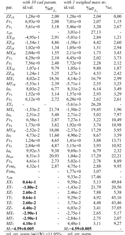
THE ESSENTIAL DYNAMIC PARAMETERS OF THE TX-40IDENTIFIED WITH IDIM-TLS.

par. id.val. ˆ % ri    id.val. % _ˆ ri   %ei ZZ1R 1,28e+0 2,00 1,28e+0 2,04 0,00 Fv1 6,93e+0 2,08 7,01e+0 2,07 1,15 Fs1 5,61e+0 3,18 5,46e+0 3,20 2,67 off1 - - 3,01e-1 27,13 - XX2R -4,95e-1 2,91 -5,01e-1 2,84 1,21 XZ2R -1,54e-1 4,86 -1,58e-1 4,42 2,60 ZZ2R 1,02e+0 1,34 1,05e+0 1,51 2,94 MX2R 2,04e+0 1,55 2,11e+0 1,73 3,43 Fv2 4,29e+0 2,10 4,45e+0 2,02 3,73 Fs2 7,56e+0 2,48 7,72e+0 2,28 2,12 XX3R 1,07e-1 9,79 1,05e-1 9,80 1,87 ZZ3R 1,24e-1 5,25 1,27e-1 4,53 2,42 MX3 4,02e-2 18,36 4,14e-2 16,79 2,99 MY3R -5,53e-1 2,39 -5,71e-1 2,55 3,25 Ia3 8,03e-2 6,77 8,31e-2 6,14 3,49 Fv3 1,52e+0 3,14 1,57e+0 2,93 3,29 Fs3 6,12e+0 2,72 6,28e+0 2,62 2,61 XY4 - - -5,61e-3 26,20 - MX4 -1,53e-2 21,74 -1,50e-2 19,45 1,96 Ia4 2,51e-2 5,48 2,71e-2 5,02 7,97 Fv4 6,58e-1 2,87 7,27e-1 3,22 10,49 Fs4 1,73e+0 3,62 1,92e+0 3,74 10,98 MY5R -2,52e-2 18,08 -2,37e-2 17,29 5,95 Ia5 4,73e-2 11,60 4,90e-2 8,67 3,59 Fv5 1,24e+0 4,65 1,41e+0 3,88 13,71 Fs5 2,84e+0 4,87 3,15e+0 3,93 10,92 Ia6 9,92e-3 9,38 9,69e-3 6,79 2,32 Iam6 8,51e-3 20,93 1,04e-2 17,29 22,21 Fv6 4,61e-1 2,73 5,02e-1 2,78 8,89 Fvm6 4,32e-1 2,87 4,75e-1 2,88 9,95 Fsm6 - - 1,77e+0 3,07 - off6 - - 9,33e-2 17,46 - XX7 0.64e-1 - 9,59e-2 5,13 49,84 XY7 -1.80e-2 - -1,43e-2 21,79 20,56 XZ7 2.60e-2 - 2,46e-2 7,88 5,38 YY7 0.64e-1 - 9,29e-2 4,92 45,16 YZ7 2.60e-2 - 3,73e-2 4,48 43,46 ZZ7 4.40e-2 - 6,03e-2 3,41 37,05 MX7 -2.90e-1 - -2,75e-1 2,65 5,17 MY7 -2.90e-1 - -2,84e-1 2,75 2,07 MZ7 4.10e-1 - 4,48e-1 3,11 9,27 M7=4.59±0.005 M7=4.59±0.005 -

rel. err. norm ||ρ||/||Y|| =11.95% rel. err. norm ||ρ||/||Y||=11.15% , ˆ (% ) : 8.28%,_i _{a b} mean e Y V g _ _ 1 2 1 ˆ ˆ ˆ %e_i  _i _i / _i %., where _ˆ1 i

 is the i-th parameter of IDIM-TLS using the knowledge of the ten payload parameters and _ˆ2

i

(23)

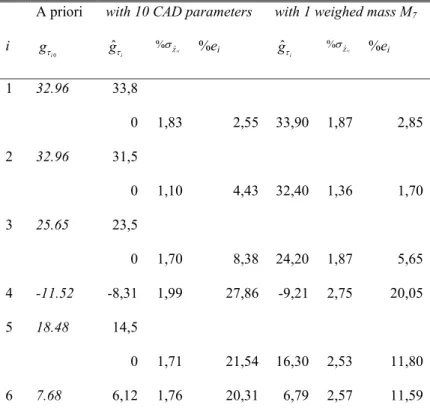
M. Gautier, S. Briot 22 Paper DS-13-1373 TABLEIV

IDIM-TLS.

A priori with 10 CAD parameters with 1 weighed mass M7

i 0 i g_ ˆ i g_ %ˆ_ri %ei ˆ i g_ %ˆri %ei 1 32.96 33,8 0 1,83 2,55 33,90 1,87 2,85 2 32.96 31,5 0 1,10 4,43 32,40 1,36 1,70 3 25.65 23,5 0 1,70 8,38 24,20 1,87 5,65 4 -11.52 -8,31 1,99 27,86 -9,21 2,75 20,05 5 18.48 14,5 0 1,71 21,54 16,30 2,53 11,80 6 7.68 6,12 1,76 20,31 6,79 2,57 11,59 (% ) :14.18%_i mean e mean(% ) : 8.94%e_i ˆ % ri 

0 0 ˆ % / % i i i i e  g_ g_ g_ .

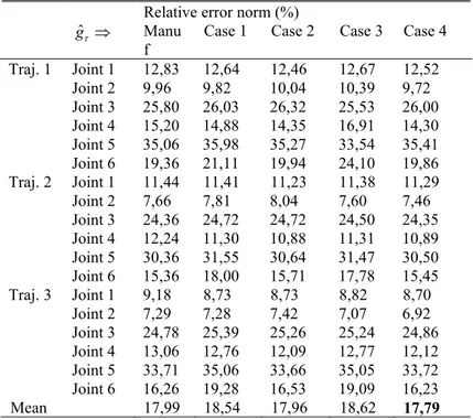
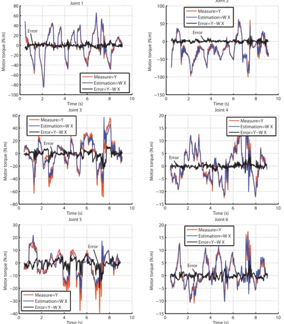
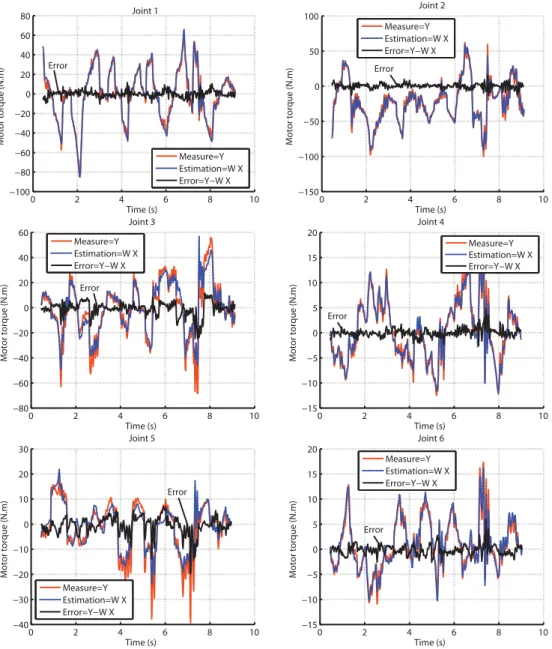
For each experiment, the relative error norms ||_ρj|| / ||_Yj ||_{computed on each joint}_{j equation} are given in Table VI. Results show that the best reconstruction is achieved for parameters of Case 4, i.e. with parameters identified with IDIM-TLS techniques considering the knowledge of

the payload mass only. In Figure 2, using the parameters identified in Case 4 of Section IV.B, the

(24)

measured motor current reference and ˆg the vector of the identified drive gains) are compared _

with torques computed using the IDIM (2) τ IDMχ (where ˆχ are the identified dynamic  ˆ

parameters). It can be observed that the torques are well calculated using the identified IDIM. It

should be mentioned that the relative errors for joints 3 and 5 are a bit higher due to unmodelled phenomena (backlash in gearboxes and non-linear friction terms).

Then, using the data collected on each trajectory, the payload is estimated using a classical

IDIM-WLS [18] presented in Sections II.C and II.D, in which the actuator torques are calculated

with the relation (4) τ v g which requires the knowledge of the drive gains. Five different  _{ }ˆ

values of ˆg are thus considered, which are the ones defined in the five previous cases (a priori _

gains or gains identified using the techniques presented in Section III). The results are given in Table VII. Only the payload mass is shown, as it is the only payload parameter value which we can trust, because it is accurately weighed.

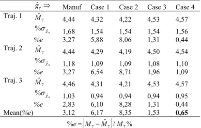
It can be observed that the best payload estimation is obtained for drive gains identified in Case

4 (%e=0.65%), i.e. with IDIM-TLS techniques considering the knowledge of the payload mass

only. The worst results are obtained for the gains identified in Cases 1 and 2 (%e=8.35%), i.e. the

gains obtained with the modified IDIM-WLS procedure. Indeed, as mentioned previously, the

noises in YL and Wr of (16) are correlated. Such correlation introduces a bias in the results and leads to wrong estimation of the parameters. In order to definitely validate our method, a second payload of 1.686±0.005 kg is attached on the end-effector and the same experiments are performed. Then, using the data collected on each trajectory, the payload is estimated using a classical IDIM-WLS [18], in which the actuator torques are calculated with the relation (4)

ˆ

 



τ v g . The same five different values of ˆg are considered. The results are given in Table _

(25)

M. Gautier, S. Briot 24 Paper DS-13-1373 TABLEV

CONDITION NUMBER OF THE OBSERVATION MATRIX

Traj. 1 Traj. 2 Traj. 3 cond(W) 2177 2817 1930

TABLEVI

RELATIVE ERROR NORMS ON TORQUE ESTIMATION FOR CROSS-VALIDATION TRAJECTORIES

Relative error norm (%) ˆg  Manu

f

Case 1 Case 2 Case 3 Case 4 Traj. 1 Joint 1 12,83 12,64 12,46 12,67 12,52 Joint 2 9,96 9,82 10,04 10,39 9,72 Joint 3 25,80 26,03 26,32 25,53 26,00 Joint 4 15,20 14,88 14,35 16,91 14,30 Joint 5 35,06 35,98 35,27 33,54 35,41 Joint 6 19,36 21,11 19,94 24,10 19,86 Traj. 2 Joint 1 11,44 11,41 11,23 11,38 11,29 Joint 2 7,66 7,81 8,04 7,60 7,46 Joint 3 24,36 24,72 24,72 24,50 24,35 Joint 4 12,24 11,30 10,88 11,31 10,89 Joint 5 30,36 31,55 30,64 31,47 30,50 Joint 6 15,36 18,00 15,71 17,78 15,45 Traj. 3 Joint 1 9,18 8,73 8,73 8,82 8,70 Joint 2 7,29 7,28 7,42 7,07 6,92 Joint 3 24,78 25,39 25,26 25,24 24,86 Joint 4 13,06 12,76 12,09 12,77 12,12 Joint 5 33,71 35,06 33,66 35,05 33,72 Joint 6 16,26 19,28 16,53 19,09 16,23 Mean 17,99 18,54 17,96 18,62 17,79

(26)

M. Gautier, S. Briot 25 Paper DS-13-1373 TABLEVII

ESTIMATION OF THE PAYLOAD MASS OF 4.59 KG ±0.005 KG

ˆg_  _{Manuf Case 1 Case 2 Case 3 Case 4} Traj. 1 7 ˆ M _{4,44 4,32 4,22 4,53 4,57} ˆ % ri   _{1,68 1,54 1,54 1,54 1,56} %e 3,27 5,88 8,06 1,31 0,44 Traj. 2 7 ˆ M _{4,44 4,29 4,19 4,50 4,54} ˆ % ri   _{1,18 1,09 1,09 1,08 1,10} %e 3,27 6,54 8,71 1,96 1,09 Traj. 3 7 ˆ M _{4,46 4,31 4,21 4,53 4,57} ˆ % ri   _{1,03 0,94 0,94 0,94 0,95} %e 2,83 6,10 8,28 1,31 0,44 Mean(%e) 3,12 6,17 8,35 1,53 0,65 7 ˆ7 7 %e M M /M % TABLEVIII

ˆg_  Manu_f _{Case 1} _{Case 2} _{Case 3 Case 4} Traj. 1 7 ˆ M _1,67 _1,58 _1,55 _1,66 1,68 ˆ % ri   _{2,61 2,51 2,51 2,49 2,53} %e 0,95 6,29 8,07 1,54 0,36 Traj. 2 7 ˆ M _{1,70 1,60 1,56 1,68 1,70} ˆ % ri   _{1,92 1,87 1,87 1,86 1,88} %e 0,83 5,10 7,47 0,36 0,83 Traj. 3 7 ˆ M _{1,70 1,59 1,56 1,67 1,70} ˆ % ri   _{1,94 1,89 1,89 1,88 1,89} %e 0,83 5,69 7,47 0,95 0,83 Mean(%e) 0.87 5,69 7,67 0,95 0,67 7 ˆ7 7 %e M M /M %

Once again, it can be observed that the best payload estimation is obtained for drive gains identified in Case 4 (%e=0.67%), i.e. with IDIM-TLS techniques considering the knowledge of

(27)

the payload mass only. This result is very close to the one obtained with the mass used for the identification (%e=0.65% in Table VII), i.e. the identified gains make the identification not

sensitive to the added mass. And the worst results are obtained for the gains identified in Cases 1 and 2, i.e. the gains obtained with the modified IDIM-WLS procedure which lead to a biased

parameter estimation.

All these results show the effectiveness of this approach: for calibrating the drive gains, it is only necessary to weigh the payload mass and to carry out standard trajectories of industrial robot. And the calibration of the drive gains improves the torques estimation and parameters identification.

To conclude this section, and in order to strengthen the method validation, we would like to mention that the proposed method has been experimentally tested on two other industrial robots (the Staübli RX-90 robot (about 10kg of payload) and the Kuka KR270 robot (270kg of payload)) and on two prototypes of parallel robots developed in French laboratories (the Orthoglide from the IRCCyN of Nantes [31] and the DualV from the LIRMM of Montpellier [32]). Experimental results have shown significant improvements of the identification of the drive gains values leading to better payload estimations for all these robots compared to the manufacturer’s values.

V. CONCLUSION

This paper has presented a new method for the global identification of the robot dynamic parameters including the gains of the total drive chain. This method is easy to implement and does not need any special test or measurement on the components of the joint drive train. It is based on an IDIM-TLS technique using motor current reference and joint position sampled data

(28)

while the robot is tracking some reference trajectories without load fixed on the robot and some trajectories with a known payload fixed on the robot end-effector. The ten inertial parameters are measured or calculated by CAD software. The method has been successfully experimentally validated on a Stäubli TX-40 robot.

0 2 4 6 8 10 −100 −80 −60 −40 −20 0 20 40 60 80 Time (s) Motor torque (N.m) Joint 1 Measure=Y Estimation=W X Error=Y−W X Error 0 2 4 6 8 10 −150 −100 −50 0 50 100 Time (s) Motor torque (N.m) Joint 2 Measure=Y Estimation=W X Error=Y−W X Error 0 2 4 6 8 10 −80 −60 −40 −20 0 20 40 60 Time (s) Motor torque (N.m) Joint 3 Measure=Y Estimation=W X Error=Y−W X Error 0 2 4 6 8 10 −15 −10 −5 0 5 10 15 20 Time (s) Motor torque (N.m) Joint 4 Measure=Y Estimation=W X Error=Y−W X Error 0 2 4 6 8 10 −40 −30 −20 −10 0 10 20 30 Time (s) Motor torque (N.m) Joint 5 Measure=Y Estimation=W X Error=Y−W X Error 0 2 4 6 8 10 −15 −10 −5 0 5 10 15 20 Time (s) Motor torque (N.m) Joint 6 Measure=Y Estimation=W X Error=Y−W X Error

Fig. 2. Motor torques (joint side units) calculated with identified gains (red) and with IDIM

(29)

Four methods have been tested: (i) a modified IDIM-WLS using ten payload parameters

calculated with CAD, (ii) the same modified IDIM-WLS using only accurately weighed payload

mass, (iii) the TLS using ten payload parameters calculated with CAD and (iv) the IDIM-TLS using only accurately weighed payload mass. Then, using the manufacturer’s drive gains and

the identified ones, results have been compared in terms of torque reconstruction and payload parameter estimation. The best results have been obtained when the IDIM-TLS is performed with

the weighed payload mass only while modified IDIM-WLS techniques gave the poorest results

due to noise correlations between the observation matrix and the measurement vector.

This approach is very simple to perform and the experimental results have shown its effectiveness: for calibrating the joint drive gains, it is only necessary to accurately weigh the payload mass and to carry standard trajectories of industrial robot.

ACKNOWLEDGEMENTS

This work was supported in part by the French FUI project IRIMI (F1004026 Z) and by the French ANR project ARROW (ANR 2011BS3 006 01).

REFERENCES

[1] Canudas de Wit, C., and Aubin, A., 1990, “Parameters identification of robots manipulators via sequential hybrid estimation algorithms”, Proc. IFAC Congress, Tallin, pp. 178-183.

[2] Gautier, M., and Poignet, P., 2001, “Extended Kalman filtering and weighted least squares dynamic identification of robot,” Control Engineering Practice, 9, pp. 1361-1372.

(30)

[3] Antonelli, G., Caccavale, F., and Chiacchio, P., 1999, “A systematic procedure for the identification of dynamic parameters of robot manipulators,” Robotica, 17(4), pp. 427-435.

[4] Kozlowski, K., 1998, “Modelling and identification in robotics”. Springer, London.

[5] Hollerbach, J., Khalil, W., and Gautier, M., 2008, “Model Identification”, chapter 14 in Siciliano, B., and Khatib, O., Eds. Springer Handbook of Robotics, Springer.

[6] Khalil, W., and Dombre, E., 2002, “Modeling, identification and control of robots”,

Hermes Penton London.

[7] Khosla, P.K., and Kanade, T., 1985, “Parameter identification of robot dynamics”, Proc. 24th_{IEEE CDC, Fort-Lauderdale, pp. 1754-1760.}

[8] Lu, Z., Shimoga, K.B., and Goldenberg, A., 1993, “Experimental determination of dynamic parameters of robotic arms”, Journal of Robotics Systems, 10(8), p. 1009-1029.

[9] Restrepo, P.P., and Gautier, M., 1995, “Calibration of drive chain of robot joints,”

Proceedings of the 4th IEEE Conference on Control Applications, pp. 526-531.

[10] Corke, P., 1996, “In situ measurement of robot motor electrical constants,” Robotica,

23(14), pp.433–436.

[11] Gautier, M., and Briot, S., 2011, “New Method for Global Identification of the Joint Drive Gains of Robots using a Known Inertial Payload”, Proc. IEEE ECC CDC, December

12-15, Orlando, Florida, USA.

[12] Gautier, M., and Briot, S., 2011, “New Method for Global Identification of the Joint Drive Gains of Robots using a Known Payload Mass”, Proc. IEEE IROS., Sept., San Fran., USA.

[13] Gautier, M., and Briot, S., 2012, “Global Identification of Drive Gains Parameters of Robots Using a Known Payload”, Proc. IEEE ICRA, May, Saint Paul, MI, USA.

(31)

[14] Hamon, P., Gautier, M., and Garrec, P., 2011, “New Dry Friction Model with Load- and Velocity-Dependence and Dynamic Identification of Multi-DOF Robots,” Proceedings of the IEEE International Conference on Robotics and Automation, Shanghai, pp. 1077-1084.

[15] Mayeda,H., Yoshida, K., and Osuka, K., 1990, “Base parameters of manipulator dynamic models”, IEEE Trans. on Robotics and Automation, 6(3), pp. 312-321.

[16] Gautier, M., and Khalil, W., 1990 “Direct calculation of minimum set of inertial parameters of serial robots,” IEEE Trans. on Robotics and Automation, 6(3), pp. 368-373.

[17] Gautier, M., 1991, “Numerical calculation of the base inertial parameters”, Journal of Robotics Systems, 8(4), pp. 485-506.

[18] Khalil, W., Gautier, M., and Lemoine, P., 2007, “Identification of the payload inertial parameters of industrial manipulators,” Proc. IEEE ICRA, Roma, Italy, April 10-14, pp.

4943-4948.

[19] Gautier,M.,1997,“Dynamic identification of robots with power model”,Proc. IEEE ICRA,

Albuquerque, USA, April, pp. 1922-1927.

[20] Kavanagh, R.C., 2001, “Performance analysis and compensation of M/T-type digital tachometers,” IEEE Transactions on Instrumentation and Measurement, 50(4), pp.

965-970.

[21] Swevers, J., Ganseman, C., Tukel, D., DeSchutter, J., and Van Brussel, H., 1997, “Optimal robot excitation and identification,” IEEE Trans. on Robotics and Automation, 13, pp.

730-740.

[22] Presse, C., and Gautier, M., 1993, “New criteria of exciting trajectories for robot identification. Proc. IEEE ICRA, pp. 907-912.

(32)

[23] Rao, C.R., and Toutenburg, H., 1999, “Linear Models: Least Squares and Alternatives, Second Edition”, Springer Series in Statistics.

[24] Van Huffel, S., and Vandewalle, J., 1991, “The Total Least Squares Problem: Computational Aspects and Analysis.” Frontiers in Applied Mathematics series, 9.

Philadelphia, Pennsylvania: SIAM.

[25] Markovsky, I., and Van Huffel, S., 2007, “Overview of total least-squares methods,” Signal Processing, 87, pp. 2283–2302.

[26] Markovsky, I., Sima, D. M., and Van Huffel, S., 2010, “Total least squares methods”,

WIREs Computational Statistics, 2.

[27] Van Huffel, S., 1991, “The Generalized Total Least Squares Problem: Formulation, Algorithm and Properties,” Numerical Linear Algebra, Digital Signal Processing and Parallel Algorithms, NATO ASI Series, 70, pp. 651-660.

[28] Golub, G.H., and Van Loan, C.F., 1983, “Matrix computation” J. Hopkins 2nd Ed. Baltimore: Johns Hopkins University Press.

[29] Gautier, M., Vandanjon, P., and Presse, C., 1994, “Identification of inertial and drive gain parameters of robots,” Proc. IEEE CDC, Lake Buena Vista, FL, USA, pp. 3764-3769.

[30] Khalil, W., and Creusot, D., 1997, “Symoro+: a system for the symbolic modeling of robots,” Robotica, 15, pp. 153-161.

[31] Chablat, D., and Wenger, P., 2003, “Architecture Optimization of a 3-DOF Parallel Mechanism for Machining Applications, the Orthoglide”, IEEE Trans. on Robotics and Automation, 19(3), pp. 403–410.

[32] Van der Wijk, V., Krut, S., Pierrot, F., and Herder, J., 2011, “Generic Method for Deriving the General Shaking Force Balance Conditions of Parallel Manipulators with Application

(33)

to a Redundant Planar 4-RRR Parallel Manipulator,” Proceedings of the 13th World Congress in Mechanism and Machine Science, Guanajuato, Mexico, June 19-25.

(34)

List of tables

TABLEI:THE ESSENTIAL DYNAMIC PARAMETERS OF THE TX-40IDENTIFIED WITH IDIM-WLS.

TABLEII:THE DRIVE GAINS OF THE TX-40:APRIORI STAÜBLI’S DATA AND IDENTIFIED VALUES

WITH IDIM-WLS.

TABLEIII:THE ESSENTIAL DYNAMIC PARAMETERS OF THE TX-40IDENTIFIED WITH IDIM-TLS.

TABLEIV:THE DRIVE GAINS OF THE TX-40:APRIORI STAÜBLI’S DATA AND IDENTIFIED VALUES

WITH IDIM-TLS.

TABLEV:CONDITION NUMBER OF THE OBSERVATION MATRIX

TABLE VI: RELATIVE ERROR NORMS ON TORQUE ESTIMATION FOR CROSS-VALIDATION

TRAJECTORIES

TABLEVII:ESTIMATION OF THE PAYLOAD MASS OF 4.59 KG ±0.005 KG

TABLEVIII:ESTIMATION OF THE PAYLOAD MASS OF 1.686 KG ±0.005 KG

List of figures

Fig. 1. TX-40 robot and its calibrated payload of 4.59 Kg

(35)

M. Gautier, S. Briot 34 Paper DS-13-1373 Fig1.eps

(36)

M. Gautier, S. Briot 35 Paper DS-13-1373 Fig2.eps 0 2 4 6 8 10 −100 −80 −60 −40 −20 0 20 40 60 80 Time (s) Motor torque (N.m) Joint 1 Measure=Y Estimation=W X Error=Y−W X Error 0 2 4 6 8 10 −150 −100 −50 0 50 100 Time (s) Motor torque (N.m) Joint 2 Measure=Y Estimation=W X Error=Y−W X Error 0 2 4 6 8 10 −80 −60 −40 −20 0 20 40 60 Time (s) Motor torque (N.m) Joint 3 Measure=Y Estimation=W X Error=Y−W X Error 0 2 4 6 8 10 −15 −10 −5 0 5 10 15 20 Time (s) Motor torque (N.m) Joint 4 Measure=Y Estimation=W X Error=Y−W X Error 0 2 4 6 8 10 −40 −30 −20 −10 0 10 20 30 Time (s) Motor torque (N.m) Joint 5 Measure=Y Estimation=W X Error=Y−W X Error 0 2 4 6 8 10 −15 −10 −5 0 5 10 15 20 Time (s) Motor torque (N.m) Joint 6 Measure=Y Estimation=W X Error=Y−W X Error

(37)

M. Gautier, S. Briot 36 Paper DS-13-1373 TABLEI

THE ESSENTIAL DYNAMIC PARAMETERS OF THE TX-40IDENTIFIED WITH IDIM-WLS.

parameter id.val. % _ˆ ri    id.val. % _ˆ ri   %ei ZZ1R 1,17e+0 2,28 1,14e+0 2,66 2,56 Fv1 6,35e+0 2,37 6,21e+0 2,70 2,20 Fs1 5,18e+0 3,80 4,98e+0 4,10 3,86 XX2R -4,54e-1 3,53 -4,43e-1 3,81 2,42 XZ2R -1,43e-1 5,85 -1,43e-1 5,88 0,00 ZZ2R 9,85e-1 1,36 9,60e-1 1,92 2,54 MX2R 1,97e+0 1,57 1,92e+0 2,21 2,54 Fv2 4,17e+0 2,09 4,09e+0 2,52 1,92 Fs2 7,28e+0 2,60 7,09e+0 2,91 2,61 XX3R 9,56e-2 13,42 9,14e-2 13,84 4,39 ZZ3R 1,19e-1 5,50 1,16e-1 5,75 2,52 MX3 3,63e-2 24,39 3,77e-2 23,00 3,86 MY3R -5,19e-1 2,69 -5,02e-1 3,30 3,28 Ia3 7,52e-2 7,29 7,39e-2 7,44 1,73 Fv3 1,46e+0 3,22 1,42e+0 3,60 2,74 Fs3 5,81e+0 2,87 5,64e+0 3,29 2,93 XY4 - - -5,27e-3 35,04 - MX4 -1,53e-2 18,62 -1,34e-2 21,25 12,42 Ia4 2,50e-2 4,63 2,36e-2 5,55 5,60 Fv4 6,54e-1 2,49 6,37e-1 3,76 2,60 Fs4 1,72e+0 3,11 1,68e+0 4,26 2,33 MY5R -2,40e-2 14,60 -2,26e-2 15,67 5,83 Ia5 4,69e-2 8,11 4,24e-2 9,28 9,59 Fv5 1,24e+0 3,63 1,21e+0 4,56 2,42 Fs5 2,81e+0 3,87 2,71e+0 4,83 3,56 Ia6 9,80e-3 6,29 8,33e-3 7,77 15,00 Iam6 8,49e-3 19,92 8,95e-3 18,72 5,42 Fv6 4,57e-1 2,07 4,34e-1 3,51 5,03 Fvm6 4,30e-1 3,21 4,11e-1 4,31 4,42 Fsm6 1,52e+0 2,95 1,53e+0 4,11 0,66 off6 - - 7,91e-2 24,72 - XX7 0.64e-1 - 8,39e-2 5,79 31,09 XY7 -1.80e-2 - -1,19e-2 17,55 33,89 XZ7 2.60e-2 - 2,22e-2 9,69 14,62 YY7 0.64e-1 - 8,20e-2 5,82 28,13 YZ7 2.60e-2 - 3,18e-2 5,33 22,31 ZZ7 4.40e-2 - 5,21e-2 3,92 18,41 MX7 -2.90e-1 - -2,43e-1 3,29 16,21 MY7 -2.90e-1 - -2,54e-1 3,41 12,41 MZ7 4.10e-1 - 3,91e-1 3,90 4,63 M7=4.59±0.005 M7=4.59±0.005 -

rel. err. norm ||ρ||/||Y|| =12.40% rel. err. norm ||ρ||/||Y||=12.43%

, ˆ

(% ) : 7.86%,_i _{a b}

mean e Y V g  _,

1 2 1

ˆ ˆ ˆ

%e_i  _i _i / _i %., where ˆ_i1 is the i-th parameter of IDIM-WLS using the knowledge of the ten payload parameters and

2 ˆ_i

(38)

M. Gautier, S. Briot 37 Paper DS-13-1373 TABLEII

IDIM-WLS.

A priori with 10 CAD parameters with 1 weighed mass M7

i 0 i g_ ˆ i g_ % _ˆ ri   %ei ˆ i g_ % _ˆ ri   %ei 1 32.96 30,20 2,41 8,37 31,10 2,02 5,64 2 32.96 29,80 1,72 9,59 30,50 1,09 7,46 3 25.65 21,80 2,36 15,01 22,40 1,74 12,67 4 -11.52 -8,06 3,33 30,03 -8,27 1,76 28,21 5 18.48 14,00 3,10 24,24 14,40 1,36 22,08 6 7.68 5,88 3,15 23,44 6,08 1,44 20,83 (% ) :18.45%_i mean e mean(% ) :16..5%e_i ˆ % ri 

0 0 ˆ % / % i i i i e  g g g .

(39)

M. Gautier, S. Briot 38 Paper DS-13-1373 TABLEIII

THE ESSENTIAL DYNAMIC PARAMETERS OF THE TX-40IDENTIFIED WITH IDIM-TLS.

par. id.val. ˆ % ri    id.val. % _ˆ ri   %ei ZZ1R 1,28e+0 2,00 1,28e+0 2,04 0,00 Fv1 6,93e+0 2,08 7,01e+0 2,07 1,15 Fs1 5,61e+0 3,18 5,46e+0 3,20 2,67 off1 - - 3,01e-1 27,13 - XX2R -4,95e-1 2,91 -5,01e-1 2,84 1,21 XZ2R -1,54e-1 4,86 -1,58e-1 4,42 2,60 ZZ2R 1,02e+0 1,34 1,05e+0 1,51 2,94 MX2R 2,04e+0 1,55 2,11e+0 1,73 3,43 Fv2 4,29e+0 2,10 4,45e+0 2,02 3,73 Fs2 7,56e+0 2,48 7,72e+0 2,28 2,12 XX3R 1,07e-1 9,79 1,05e-1 9,80 1,87 ZZ3R 1,24e-1 5,25 1,27e-1 4,53 2,42 MX3 4,02e-2 18,36 4,14e-2 16,79 2,99 MY3R -5,53e-1 2,39 -5,71e-1 2,55 3,25 Ia3 8,03e-2 6,77 8,31e-2 6,14 3,49 Fv3 1,52e+0 3,14 1,57e+0 2,93 3,29 Fs3 6,12e+0 2,72 6,28e+0 2,62 2,61 XY4 - - -5,61e-3 26,20 - MX4 -1,53e-2 21,74 -1,50e-2 19,45 1,96 Ia4 2,51e-2 5,48 2,71e-2 5,02 7,97 Fv4 6,58e-1 2,87 7,27e-1 3,22 10,49 Fs4 1,73e+0 3,62 1,92e+0 3,74 10,98 MY5R -2,52e-2 18,08 -2,37e-2 17,29 5,95 Ia5 4,73e-2 11,60 4,90e-2 8,67 3,59 Fv5 1,24e+0 4,65 1,41e+0 3,88 13,71 Fs5 2,84e+0 4,87 3,15e+0 3,93 10,92 Ia6 9,92e-3 9,38 9,69e-3 6,79 2,32 Iam6 8,51e-3 20,93 1,04e-2 17,29 22,21 Fv6 4,61e-1 2,73 5,02e-1 2,78 8,89 Fvm6 4,32e-1 2,87 4,75e-1 2,88 9,95 Fsm6 - - 1,77e+0 3,07 - off6 - - 9,33e-2 17,46 - XX7 0.64e-1 - 9,59e-2 5,13 49,84 XY7 -1.80e-2 - -1,43e-2 21,79 20,56 XZ7 2.60e-2 - 2,46e-2 7,88 5,38 YY7 0.64e-1 - 9,29e-2 4,92 45,16 YZ7 2.60e-2 - 3,73e-2 4,48 43,46 ZZ7 4.40e-2 - 6,03e-2 3,41 37,05 MX7 -2.90e-1 - -2,75e-1 2,65 5,17 MY7 -2.90e-1 - -2,84e-1 2,75 2,07 MZ7 4.10e-1 - 4,48e-1 3,11 9,27 M7=4.59±0.005 M7=4.59±0.005 -

rel. err. norm ||ρ||/||Y|| =11.95% rel. err. norm ||ρ||/||Y||=11.15% , ˆ (% ) : 8.28%,_i _{a b} mean e Y V g _ _ 1 2 1 ˆ ˆ ˆ

%e_i  _i _i / _i %., where ˆ_i1 is the i-th parameter of IDIM-TLS using the knowledge of the ten payload parameters and ˆ_i2 is the i-th parameter of IDIM-TLS using the knowledge of the payload mass only.

(40)

M. Gautier, S. Briot 39 Paper DS-13-1373 TABLEIV

IDIM-TLS.

A priori with 10 CAD parameters with 1 weighed mass M7

i 0 i g_ ˆ i g_ %ˆ_ri %ei ˆ i g_ %ˆri %ei 1 32.96 33,8 0 1,83 2,55 33,90 1,87 2,85 2 32.96 31,5 0 1,10 4,43 32,40 1,36 1,70 3 25.65 23,5 0 1,70 8,38 24,20 1,87 5,65 4 -11.52 -8,31 1,99 27,86 -9,21 2,75 20,05 5 18.48 14,5 0 1,71 21,54 16,30 2,53 11,80 6 7.68 6,12 1,76 20,31 6,79 2,57 11,59 (% ) :14.18%_i mean e mean(% ) : 8.94%e_i ˆ % ri 

0 0 ˆ % / % i i i i e  g_ g_ g_ .

(41)

M. Gautier, S. Briot 40 Paper DS-13-1373 TABLEV

CONDITION NUMBER OF THE OBSERVATION MATRIX

Traj. 1 Traj. 2 Traj. 3 cond(W) 2177 2817 1930

(42)

M. Gautier, S. Briot 41 Paper DS-13-1373 TABLEVI

RELATIVE ERROR NORMS ON TORQUE ESTIMATION FOR CROSS-VALIDATION TRAJECTORIES

Relative error norm (%) ˆg_  Manu

f

Case 1 Case 2 Case 3 Case 4 Traj. 1 Joint 1 12,83 12,64 12,46 12,67 12,52 Joint 2 9,96 9,82 10,04 10,39 9,72 Joint 3 25,80 26,03 26,32 25,53 26,00 Joint 4 15,20 14,88 14,35 16,91 14,30 Joint 5 35,06 35,98 35,27 33,54 35,41 Joint 6 19,36 21,11 19,94 24,10 19,86 Traj. 2 Joint 1 11,44 11,41 11,23 11,38 11,29 Joint 2 7,66 7,81 8,04 7,60 7,46 Joint 3 24,36 24,72 24,72 24,50 24,35 Joint 4 12,24 11,30 10,88 11,31 10,89 Joint 5 30,36 31,55 30,64 31,47 30,50 Joint 6 15,36 18,00 15,71 17,78 15,45 Traj. 3 Joint 1 9,18 8,73 8,73 8,82 8,70 Joint 2 7,29 7,28 7,42 7,07 6,92 Joint 3 24,78 25,39 25,26 25,24 24,86 Joint 4 13,06 12,76 12,09 12,77 12,12 Joint 5 33,71 35,06 33,66 35,05 33,72 Joint 6 16,26 19,28 16,53 19,09 16,23 Mean 17,99 18,54 17,96 18,62 17,79

(43)

M. Gautier, S. Briot 42 Paper DS-13-1373 TABLEVII

ˆg_  _{Manuf Case 1 Case 2 Case 3 Case 4} Traj. 1 7 ˆ M _{4,44 4,32 4,22 4,53 4,57} ˆ % ri   _{1,68 1,54 1,54 1,54 1,56} %e 3,27 5,88 8,06 1,31 0,44 Traj. 2 7 ˆ M _{4,44 4,29 4,19 4,50 4,54} ˆ % ri   _{1,18 1,09 1,09 1,08 1,10} %e 3,27 6,54 8,71 1,96 1,09 Traj. 3 7 ˆ M _{4,46 4,31 4,21 4,53 4,57} ˆ % ri   _{1,03 0,94 0,94 0,94 0,95} %e 2,83 6,10 8,28 1,31 0,44 Mean(%e) 3,12 6,17 8,35 1,53 0,65 7 ˆ7 7 %e M M /M %