HAL Id: hal-00553090
https://hal.archives-ouvertes.fr/hal-00553090
Submitted on 25 Jun 2019
HAL is a multi-disciplinary open access
archive for the deposit and dissemination of sci-entific research documents, whether they are pub-lished or not. The documents may come from teaching and research institutions in France or abroad, or from public or private research centers.
L’archive ouverte pluridisciplinaire HAL, est destinée au dépôt et à la diffusion de documents scientifiques de niveau recherche, publiés ou non, émanant des établissements d’enseignement et de recherche français ou étrangers, des laboratoires publics ou privés.
for the Computation of their Natural Frequencies
Sébastien Briot, Anatol Pashkevich, Damien Chablat
To cite this version:
Sébastien Briot, Anatol Pashkevich, Damien Chablat. Reduced Elastodynamic Modelling of Parallel Robots for the Computation of their Natural Frequencies. 13th World Congress in Mechanism and Machine Science, Jun 2011, Guanajuato, Mexico. �hal-00553090�
1
Reduced Elastodynamic Modelling of Parallel Robots for the Computation of
their Natural Frequencies
S. Briot* A. Pashkevich† D. Chablat‡
IRCCyN – CNRS
Nantes, France IRCCyN – CNRS / Ecole des Mines de Nantes Nantes, France IRCCyN – CNRS Nantes Nantes, France
Abstract— In this paper is presented an approach for computing the first natural frequencies of parallel robots. This approach, based on the Rayleigh-Ritz approximation, aims at reducing the model dimension by decreasing the size of the matrices describing the robot mass and stiffness, saving computational time and avoiding inaccuracy due to ill-conditioning. Thus it can be used in the design procedure as well as in real-time control. Simulations are carried out on a PRRRP robot modelled in 3D and comparisons with FEA software are presented.
Keywords: elastodynamic modelling, model dimension reduction, natural frequencies, parallel robots.1
I Introduction
Parallel robots have increasingly been used in industry in the last few years, mainly for pick-and-place applications or high-speed machining [1], [2]. This interest is due to their main properties, i.e. their higher rigidity and dynamic capacities compared with their serial manipulator counterparts.
Having a good knowledge of the elastodynamic behaviour of a manipulator (especially its natural frequencies) is a crucial point. In this sense, accurate elastodynamic models are necessary at both the control stage [3]–[5] and design stage [6]–[8], in order to optimize the geometry, as well as the shape of the elements of the manipulator. This will lead to the creation of a mechanism in which vibrations will be minimized.
Several models have been proposed and used in the literature in order to compute the natural frequencies of a mechanism during a preliminary design. Three main general methods can be distinguished:
Finite element analysis (FEA); the FEA method is proved to be the most accurate and reliable, since the links/joints are modeled with its true dimension and shape [7], [9]–[12]. Its accuracy is limited by the discretization step only. However, because of high computational expenses required for the repeated re-meshing, this method is usually applied at the final
*Sebastien.Briot@irccyn.ec-nantes.fr
†Anatol.Pashkevich@emn.fr
‡Damien.Chablat@irccyn.ec-nantes.fr
1 13th World Congress in Mechanism and Machine Science,
Guanajuato, México, 19-25 June, 2011
design stage for the verification and component dimensioning.
Matrix structural analysis (MSA) method is a common technique in mechanical engineering [13], [14]; it incorporates the main ideas of the FEA but operates with rather large flexible elements (beams, arcs, cables, etc.). This obviously yields reduction of the computational expense and, in some cases, allows analytical stiffness matrix to be obtained. However, this method can only be applied to links with simple shapes and requires improved skills in FEA.
Virtual joint methods (VJM) [8], [15], which is also referred to as ‘‘lumped modelling”, is based on the expansion of the traditional rigid model by adding virtual joints (localized springs), which describe the elastic deformations of the manipulator components (links, joints and actuators). Such kind of modelling is well adapted for links with complex shapes [16]. Generally, lumped modelling is simpler to use than MSA and provides acceptable accuracy in reduced computational time. It is widely used at the pre-design stage, especially for the analytical parametric analysis. However, due to the large number of virtual joints that have to be modelled in order to obtain good accuracy, such an approach is time-consuming. Moreover, for closed-loop mechanisms with passive joints, the way to assemble the matrices and to model the passive joints in kinematic chains is not straightforward.
The purpose of this paper is to propose a reduced elastodynamic modelling approach on parallel robots for the computation of the natural frequencies only, based on VJM. By keeping the simplicity of use of the VJM, this modelling considerably decreases the dimension of the problem by inverting only 6×6 matrices. It also proposes a straightforward procedure for the modelling of passive joints on parallel robots and for the assembly of the mass and stiffness matrices of closed-loop structures.
This paper will be organised as follows. Section 2 presents the theoretical background necessary in order to reduce the size of the elastodynamic model for the computation of the natural frequencies. In section 3, a numerical example is proposed in order to show the efficiency of our method. Finally, conclusions are drawn in section 4.
2 II. Theoretical background
A. Problem statement
Let us consider a general parallel manipulator made of n legs, each leg being composed of m links, m passive and one active joints, considered as ideal, i.e. without friction (Fig. 1a). Using the basic idea of VJM [15], let us decompose the j-th link of the i-th leg (denoted as the link ij where j = 1, 2, …, m and i = 1, 2, …, n) into pij
rigid elements and virtual springs (Fig. 1b). The mass and inertia matrix of the k-th rigid element of link ij (denoted as the element ijk) expressed in the local frame attached to this element, are denoted as mijk and Iijk, respectively.
The displacement of its centre of mass Sijk expressed in
the base frame, resulting from the robot deformations, is denoted as [ 1, 2,..., 6]T
ijk qijk qijk qijk
0q 0 0 0 , where the first
three components of this vector correspond to the translational displacements along the x, y and z axes of the base frame, respectively, and the last three components to the rotational displacements along the same axes. It should be mentioned that in the remainder of the paper, the left superscript “0” will stand for the coordinates expressed in the global frame. If no left superscript is mentioned, the vector is expressed in the local frame attached to the link ij.
The deformations of the k-th spring of link ij (denoted as the spring ijk) are denoted as [ 1, 2,..., 6]T
ijk ijk ijk ijk
θ ,
where the three first components of this vector correspond to the translational deformations along the x,
y and z axes of the base frame, respectively, and the last three components to the rotational deformations along the same axes. The kinetic energy of the system is equal to:
1 1 1 1 1 2 2 ij p n m T T
ijk ijk ijk tot i j k
T
0q 0M 0q q M q (1)where 0 ijk diag(mijk ,0 ijk) 3
M I I , I3 being the identity
matrix of dimension 3, [ 111T , 112T ,..., T nm]T nmp
0 0 0
q q q q is
the vector regrouping all vectors 0qijk (i.e. the velocity of
the centre of masses Sijk) and Mtot is the global mass
matrix of the system.
The potential (elastic) energy of the system is equal to:
1 1 1 1 2 ij p n m T e ijk ijk ijk
i j k
V
θ K θ (2)where Kijk is the stiffness matrix of the virtual spring ijk.
It is shown in [8], [15] that the deformations θijk can be related to the displacements of the centres of masses of elements ijk and ij(k+1) by the relation:
2, 1, ( 1) ( 1) ijk ijk ijk ij k ij k 0 0 q θ C C q (3)
where C2,ijk and C1,ij(k+1) are two 6 by 6 matrices. Therefore, (2) can be rewritten as:
2, 2, ( 1) 1, 1 1, 1 ( 1) , , 1 1 2 2 T T T T ijk k k ijk T e T T ijk T tot ij k k k ij k i j k V
00 00 q C C q K q K q q C C q (4)(a) Architectural representation
(b) Elastic representation of one link Fig. 1. A general parallel manipulator.
where [ 111T , 112T ,..., T nm]T nmp
0 0 0
q q q q is the vector
regrouping all vectors 0qijk and K
tot is the global stiffness
matrix of the system.
Starting from these definitions, and considering that the robot is in an equilibrium position and no external forces are applied, the authors of [15] demonstrate that the system is governed by the relation:
tot tot
M q K q 0 . (5)
A solution ql of this equation can be found by solving
the system:
2
l tot tot l
M K q 0, with l2fl (6)
where ql represents the vectors of the shape of free
vibrations of the system for the l-th natural mode, fl and
l are their corresponding natural frequency and
pulsation, respectively. If the matrix 2
l tot tot
M K is singular (which is always the case when l is one of the modal pulsation of
the robot), ql becomes non-null and is the eigenvector
corresponding to the pulsation l. There is an infinity of
vectors ql validating (6) (for a given l), but all are
proportional to the others. Vector ql is not necessarily
dependent of time, but almost represents the amplitude of the vibrations. Therefore, when only the l-th mode of the system is excited, the displacements of all springs may be written under the form:
* sin( )
l l ltl
3
where l is a phase difference corresponding to the mode l. When all modes are excited, the displacement q of all
spring centres may be written in the form:
6 6 * 1 1 sin( ) d d l l l l l l t
q q q (8)The most common way to find the values of the pulsation l is to solve the eigenvalue problem
2 1
det lI M K tot tot 0. (9)
where I is an identity matrix of dimension 6 d, with d = ,
ij i j
n m
p .However, solving this problem involves finding the 6
d eigenvalues of the problem and also inverting the d
matrices M constituting the matrix Mijk tot, which is
highly time-consuming and can lead to few accurate results because of the problem dimension.
In order to avoid such kind of drawbacks [16] has recently proposed (for elastostatic modelling only) a new procedure to compute the deformations of the robot when a force is applied at the end-effector. This procedure computes a stiffness (and also compliance) matrix Kr
(and Sr, resp.) of dimension 6 that represents the
behaviour of the robot in terms of deformations. Moreover, during the procedure, only inversions of 6 dimensional matrices are involved, which considerably reduces computational time and avoids accuracy problems due to ill-conditioning of the large global stiffness matrix. Thus, the global 6 d dimensional problem defined with respect to all variables q has been
reduced to a 6 dimensional problem defined with respect to platform deflections t only. As a result, the entire robot can locally be seen as a virtual spring of dimension 6 that deforms when applying a wrench on the end-effector.
Starting from these considerations, it would be interesting to reduce the dimension of the problem by expressing Eq. (6) as a function of the reduced stiffness matrix Kr, of the platform deflections t and, also, as a
function of a reduced mass matrix that will be denoted as
Mr, which could represent the global behaviour of the
robot in terms of natural frequencies. The remainder of the paper will focus on this problem.
B. Rayleigh-Ritz approximation
Another way to find the natural pulsation l of the
mode l would be to know the exact amplitude l of the
displacements ql for this mode. For the natural mode l,
the potential and kinetic energies of the system are given by:
* * 2 1 1 sin 2 2 T T e l tot l l tot l l l V q K q q K q t (10a)
* * 2 2 1 1 cos 2 2 T T l tot l l l tot l l l T q M q q M q t (10b)From the principle of energy conservation, it follows that
max Ve max T 0, i.e T
2
0l l tot tot l
q M K q (11)
which is an univariate equation in l.
It is obvious that the exact knowledge of the amplitude
ql is an impossible task without a direct measure on the
system of all the displacements of the robot nodes. However, this vector may be approximated by another denoted as qˆl that is close to the exact amplitude ql.
Introducing this approximated vector qˆl into (10) will allow us to find a corresponding value of and, as a ˆl
result, fˆl which is the approximated natural frequency of
the system. Such kind of elastodynamic problem resolution is called the Rayleigh-Ritz method [17].
The better the approximation, the more accurate the value of . The designer’s skills in terms of ˆl
understanding and analysis of robot physical behaviour here are of the utmost importance. In this sense, let us recall that the first natural frequencies are associated with the highest level of energy due to vibrations, and represent the highest displacements of the structure. Therefore, in design optimization loops, it is essential to maximize the value of the first frequency.
Using the Rayleigh-Ritz approximation in order to compute the first natural frequencies, the stresses for which the maximal displacements appear have to be found. From our experience in elastic behaviour of robots, it is assumed that a good approximation of these maximal displacements will be the deformation of the robot with a load applied at the end-effector, and it can be shown in the following that this hypothesis is valid. Using this assumption, the displacements ql of all springs
can be computed as a function of the end-effector displacements t, i.e. it is possible to define a matrix Jq
such as:
l q
q J δt. (12)
As a result, introducing (12) into (11) will lead to
2
T T T
l tot tot
q q q q
δt J M J J K J δt 0 (13)
where the matrices T tot q q J M J and T tot q q J K J are now of
dimension 6. It should be mentioned here that, in the case where an external load is applied at the end-effector only, the term T
tot
q q
J K J is equal to the reduced stiffness matrix
Kr of the robot. Therefore, (13) can be rewritten as:
2
T l r r δt M K δt 0, with T tot r q q M J M J (14)In the following sections it is explained how to obtain expressions (12) and (14).
C. Reduction of the link mass matrix
It is possible to decompose the previously cited task into two sub-problems. First, the displacements of each spring in the beam ij can be expressed as a function of the displacement of its extremities. Then, one can express the
4
beam extremity displacements as a function of the platform displacements t. Using this approach will allow for a reduction in the size of the link mass matrices, and thus avoiding creating global mass matrices Mtot with
very large dimension.
Two main ways can be followed to reduce the size of the link mass matrices. The first one consists in discretizing the link ij into pij rigid links and springs and
to express their displacements as a function of the beam extremity displacements. However, such numerical method must be repeated for each link and, thus, increases the size of the algorithm and decreases its efficiency. As a result, it is prefered to use the following procedure which allows analytical expressions to be obtained for the reduced link mass matrices.
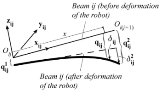
Let us consider the link ij, modelled as a beam (Fig. 2). At this beam is attached a local frame represented by the vectors xij, yij and zij. Before any deformation of the
system, the beam ij is linked (rigidly or by a passive joint) to beams i(j–1) and i(j+1) at points Oij and Oi(j+1),
respectively (Fig. 2). After deformation of the robot, the beam extremity located at Oij is displaced from
1 2 6 1 1 1 [ , ,..., ]T ij ij ij q q q 1 ij
q and the one located at Oi(j+1) is
displaced from [ 21, 22,..., 26]T ij ij ij q q q 2 ij
q , where the three
first components of each vector correspond to the translational displacements along local xij, yij and zij axes,
respectively, and the three last components to the rotational displacements along the same axes.
The general formula for the kinetic energy of an elastic Bernoulli beam is equal to [14]:
0 1 2 ij L T ij ij T
q Q qij ijijdx (15) with diag( , , , p, , )y z ij ij ij ij ij ij A A A I I I ij Q . In this expression, ijq represents the velocity of the beam cross-section
located at position x from the local reference frame (Fig. 2), Lij is the length of the beam ij, ij the mass density at
cross-section x, Aij its area, Iijp its torsional constant and y
ij
I , z
ij
I the quadratic momentums along yij and zij,
respectively.
For the l-th natural mode, and from (7), the kinetic energy can be rewritten as:
2 2 0 1 cos 2 ij L T ij l l l ij T t
q Q qij ij ijdx (16)qij being the amplitude of the displacement of the beam
cross-section located at position x from the local reference frame (Fig. 2).
In the Rayleigh-Ritz approximation, considering that the deformations due to the natural vibrations are similar to those obtained when an external load is applied at the robot end-effector only, each link of the structure will deform due to the stresses transmitted through the robot joints at points Oij. As a result, the deformations ij
Fig. 2. Displacements and elastic deformations of a beam.
of the beam cross-section (Fig. 2) can be approximated by the deformations of a tip-loaded beam, given by [14]:
diag( ,f g g f h hij ij, ij, ij, , )ij ij 2 ij ij δ δ (17) where (x L ij) 2 ij ij
δ δ represents the deformation of the beam at its tip and
( ) / ij ij f x x L , (18a) 2 3 ( ) 0.5 (3 ) / ij ij ij g x x L x L , (18b) 2 ( ) ( 0.5 ) / ij ij ij h x x L x L . (18c)
As a result, the global displacement qij of the beam
cross-section at x can be expressed as a sum of two terms: ( )x 3 1 ij ij ij 3 3 I D q q δ 0 I where ( ) 0 0 0 0 0 0 0 x x x D (19)
In this sum, the left terms corresponds to the displacement of the undeformed beam due to the displacement of the node located at Oij.
In the hypothesis that the beam cross-section is constant, introducing (17) and (19) into (16), and integrating, leads to:
2 2 1 cos 2 T T ij l l l T t 1 ij 1 2 ij ij ij 2 ij q q δ M δ (20) where
T 11 12 ij ij ij 12 22 ij ij M M M M M with 2 2 0 0 0 0 0 0 0 0 0 / 2 0 0 0 / 2 0 0 0 0 0 0 0 0 / 2 0 / 3 0 0 / 2 0 0 0 / 3 ij ij ij ij ij ij ij ij p ij ij ij ij y ij ij ij ij ij ij ij ij z ij ij ij ij ij ij ij m m m L m m L I L m L m L I L m L m L I L 11 ij M (21a) / 2 0 0 0 0 0 0 3 / 8 0 0 0 0 0 0 3 / 8 0 0 0 0 0 0 / 2 0 0 0 0 11 / 40 0 2 / 3 0 0 11 / 40 0 0 0 2 / 3 ij ij ij ij p ij ij ij ij y ij ij ij ij ij ij z ij ij ij ij ij m m m I L m L I L m L I L 12 ij M (21b) 33 33 8 8 diag , , , , , 3 140 140 3 15 15 p ij ij ij ij ij ij y z ij ij ij ij ij ij m m m I L I L I L 22 ij M (21c)5
It should be mentioned that, in the case where the section of the beam is not constant, (18) to (21) are no more correct. In this case, the deformation of the beam and its kinetic energy should be obtained numerically.
From (17), it can be shown that:
(Lij) 3 2 2 1 ij ij ij 3 3 I D δ q q 0 I . (22)
which leads to:
1 1 1 6 6 ij ij ij 21 ij 2 2 2 ij 6 ij ij ij I 0 q q q E E I δ q q , (Lij) 3 21 ij 3 3 I D E 0 I (23)
Introducing (23) into (20) leads to:
2 2 1 cos 2 T T ij l l l T t 1 1 ij ij ij ij ij 2 2 ij ij q q E M E q q (24) Expressing vectors v ijq (v = 1, 2) in the base frame, (24) becomes:
2 2 1 cos 2 T red ij l l l T t 0 1 0 1 ij 0 ij ij 0 2 0 2 ij ij q q M q q (25) where 0
0 T red T ij ij 0 ij ij ij ijM R E M E R and R0ij is the
rotation matrix from the local frame of beam ij to the global frame, i.e.
0ij 0 1 1 ij ij 0 2 2 ij ij q q R q q . (26)
To show the validity of the approach, let us compare the obtained equations when they are applied on a single beam fixed at one extremity O11, i.e. 0 1q110. For the numerical example, it is considered that this beam has the following characteristics:
- length L = 1 m
- hollow circular cross-section of external diameter 40 mm and internal diameter 30 mm
- material: steel (Young modulus E = 204 GPa, Poisson coefficient = 0.3, density = 8020 kg/m3)
For such an element, beam theory gives the following expressions for the natural frequencies [17]:
- 1st natural frequency due to transverse displacements:
2 3.516 35.28 Hz 2 z tr EI f m L (27a)
where m is the mass of the beam and Iz its quadratic
momentum along z axis.
- 1st natural frequency due to longitudinal displacements:
/ (4 ) 1260.86 Hz
l
f E L (27b)
- 1st natural frequency due to torsional displacements:
/( ) (4 ) 781.95 Hz
p y z to
f I G I I L (27c)
where G is the shear modulus, Iy its quadratic momentum
along y axis and Ip its torsional constant.
Applying the previously developed equations to this case by considering that the reduced mass matrix Mr =
22 11
M is given at (21c) and the stiffness matrix Kr is
expressed in [16] as: 2 2 0 0 0 0 0 0 12 / 0 0 0 6 / 0 0 12 / 0 6 / 0 1 0 0 0 0 0 0 0 6 / 0 4 0 0 6 / 0 0 0 4 z z y y p y y z z ES EI L EI L EI L EI L GI L EI L EI EI L EI r K , (28) it is found:
- 1st natural frequency due to transversal displacements: 35.78 Hz (error of 1.4%)
- 1st natural frequency due to longitudinal displacements: 1390.30 Hz (error of 10.27%)
- 1st natural frequency due to torsional displacements: 862.23 Hz (error of 10.27%)
As a conclusion, the proposed reduced model is accurate enough for the computation of the first natural frequency due to transversal displacements, which is also the first natural frequency of the beam.
Let us now reduce the size of the total mass matrix of the robot.
D. Reduction of the robot mass matrix
Using the results of the previous section, the total kinetic energy of the system is given by:
2 2 , , 2 2 1 cos 2 1 cos 2 T red ij l l l i j i j T l l l tot T T t t
0 1ij 0 0 1ij ij 0 2 0 2 ij ij q q M q q q M q (29)with ( red, red,..., red)
tot diag 0 0 0 11 12 nm M M M M and
T, T, T, T,...,
T,
T T 0 111 0 211 0 112 0 122 0 1nm 0 2nm q q q q q q q .It is necessary to express the relationship linking all vectors 0 v
ij
q (v = 1, 2) to the end-effector displacements t. From [16], this displacement is equal to:
i i i i
θ p
δt J θ J p , (30)
where i represents the deformations of all virtual springs
of the leg i and pi the displacements of its passive joints,
and Ji and Jpi are Jacobian matrices relying these
displacements to the displacement t. These matrices can be obtained by the differentiation of the global transformation matrix Ti of the chain i including rigid,
passive and elastic coordinates [16]. The way to obtain these matrices is explained in more depth in the next section. It should be mentioned that the dimension of Jpi
is 6 by m, m being the number of passive joints of the leg, with m < 6 (because one leg of a parallel robot cannot have more than five passive degrees of freedom (DOF)).
From [16], it can also be shown that:
T
i i i i i i
θ θ θ p
6
where Sθi is a block-diagonal matrix regrouping all the
compliance matrices of each virtual springs, and fi is the
force applied on the i that involves the displacement t. The expression of fi is such as
i i
f K δt (32)
Ki being the global stiffness matrix of the leg i.
Introducing (32) into (31) leads to:
T
i i i i i i
θ θ θ p
I J S J K δt J p . (33)
Therefore, the displacements pi of the robot passive
joints due to the displacement t are equal to:
T
1 T
T
i i i i i i i i i
p p p θ θ θ tp
p J J J I J S J K δt J δt. (34)
Let us now compute the displacements 0 2 ij
q of the virtual spring located at the extremity of the link ij. This spring ij is preceded by j–1 other virtual springs and passive joints. The deformations of the j springs (including the one at the link extremity) will be denoted as ij, and the displacements of the j–1 passive joints pij,
respectively. They can be related to the displacement 0 2 ij
q
by the Jacobian matrices Jij and Jpij as
ij ij ij ij
0 2
ij θ p
q J θ J p , (35)
These matrices may be computed in a similar way to the matrices Ji and Jpi, but by considering the truncated
chain i going from the base to the virtual spring ij. The deformations ij involve constraints into the j virtual
springs of the truncated chain that are denoted as ij.
Their expressions may be found from the relationship [16]:
ij ij ij
θ
S τ θ , (36)
where Sij is a block-diagonal matrix regrouping all the compliance matrices of the j virtual springs of the truncated chain. Introducing (34) into (33) leads to:
ij ij ij ij ij
0 2
ij θ θ p
q J S τ J p . (37)
Let us consider now the entire leg i of the mechanism. The constraints i applied to the springs due to the force fi
applied on the platform are given by [16],
T ij T j i i i i T i ir j i θ θ θ τ J τ J f f τ J , (38)
where Jji corresponds to the j first columns of matrix Ji. Introducing (38) into (37), T T ij ij j i i ij ij ij ij j i i ij ij 0 2 ij θ θ θ p θ θ θ p q J S J f J p J S J K δt J p . (39)
Moreover, the passive displacements pij are known
from expression (32). Considering that Jjtpi represents the
matrix composed of the j first lines of Jtpi given at (32), it
follows that
T
ij ij j i i ij j ij q2 0 2 ij θ θ θ p tp ij q J S J K J J δt J δt. (40) Once all 0 2 ijq are found, the vectors 0 1 ij
q can be computed. Indeed, displacement 0 1
ij
q is nothing none than displacement 0qi j2( 1) plus the small deflection of the passive joint located at Oij , i.e.:
( 1) pij
0 1 0 2 0
ij i j ij
q q s (41)
where pij is the value of the displacement of the passive
joint located at Oij and 0sij is a unit screw corresponding
to its twist. Introducing (34) and (40) into (41):
* * j i j i q2 q2 q1 0 1 0 0 ij ij ij tp ij ij tp ij q J δt s J δt J s J δt J δt (42) where * j itpJ is the j-th line of matrix Jtpi given at (32).
Thus, from (40) and (42), one can express vector q given at (29) as a function t as follows:
, , , ,..., , T T T T T T T nm nm 1 2 1 2 1 2 q q q q q q 11 11 12 12 q q J J J J J J δt J δt (43) Introducing this relation into (29) will lead to:
2 2 1 cos 2 T l l l T t δt M δtr (44)where the expression of Mr is given at (14).
As a result, from (14), finding the robot natural frequencies relies on solving the 6 dimensional eigenvalues problem
2 1
det lI6M Kr r 0. (45)
Let us now apply this method using an example.
III. Case study
In this section, the example of the planar PRRRP2 manipulator with two parallel prismatic axes (Fig. 3) will be treated. Let us first compute the global 3D stiffness matrix Kr of the robot.
The method presented in [16] states that each leg may be decomposed into a sequence of rigid links and virtual 6-DOF springs, which includes:
(a) a rigid link between the manipulator base and the ith actuating joint (part of the base platform);
(b) a 1-DOF actuating joint allowing one translation i0;
(c) a rigid foot;
(d) a 6-DOF virtual spring describing the foot stiffness; (e) a 1-DOF passive R-joint at the beginning of the leg
allowing one rotation with angle ; i1
(f) a rigid leg linking the foot and the end-effector; (g) a 6-DOF virtual spring describing the leg stiffness; (h) a 1-DOF passive R-joint at the end of the leg 2 (not
for leg 1) allowing one rotation with angle 22;
(i) a rigid link from the manipulator leg to the end-effector (part of the movable platform).
From these assumptions, the matrix regrouping the stiffness matrices of all segments of the leg i has the following form [16]: Foot elt Leg i i i 6 6 6 6 K 0 K 0 K . (46)
2 In the paper, P stands for an actuated prismatic pair and R for a
7
For obtaining matrices J and pi Jθi of (31), let us now
consider the corresponding mathematical expression defining the end-effector location subject to variations of all the above defined coordinates of a single kinematic chain i may be written as follows:
1 6
1 6
1 1 1 1
Base 10 Foot 11 11 1 11 Leg 1 12 12 Tool ( ) ( ,..., ) ( ) ( ,..., ) a s r s T T V T V V T V T (47) 1 6 1 6 2 2 2 2
Base 20 Foot 21 21 1 21 Leg 2 22 22 2 22 Tool ( ) ( ,..., ) ( ) ( ,..., ) ( ) a s r s r T T V T V V T V V T (48)
where the matrix function Va( ) is an elementary
translation along y, the matrix functions Vrj( ) (j = 1, 2)
are elementary rotations around z, the spring matrix
( )
s
V is composed of six elementary transformations defined by the coordinates (ij1,...,ij6) of the virtual
joints (i, j = 1, 2). Matrices Base
i T , Foot i T and Leg i T
represents the rigid displacements of the base, foot and leg, respectively [16] (Fig. 3).
The matrix Jθi may be obtained from the derivation of
the matrix Ti with respect to the spring parameters
v ij
(v = 1 to 6), at the point ijv 0, considering that
0 ' ' ' ' 0 ' ' ' ' 0 ' 0 0 0 0 v v v iz iy ix i iz ix iy L s R ij ij ij iy ix iz ij ij p p p V T H H . (49) where the first and the third multipliers are the constant homogenous matrices which do not include the displacement , and the second multiplier corresponds ijv to the derivative of the elementary translation or rotation corresponding to . In the right-hand term, symbol “ ' ” ijv denotes the first derivative of the variables with respect to . Therefore, ijv p'ix, p' and iy p'iz (resp. , 'ix 'iyand ) correspond to the small translations along (resp. 'iz
rotations about) x, y and z axes of the extremity of the leg i due to the variation of the parameter . ijv
The Jacobians Jpi can be computed in a similar manner, but the derivatives are evaluated in the neighborhood of the “nominal” values of the passive joint coordinates corresponding to the rigid case (these ij values are obtained from the inverse kinematics).
Finally, the stiffness matrix Ki of the leg i, which
relates the deformations t to the force fi can be
computed by direct inversion of relevant 7 by 7 (8 by 8 in the case of the leg 2) matrix in the left hand side of the following equation [16] i i i T i i θ p p S J f δt J 0 p 0 ,
1 elt i T i i i θ θ θ S J K J (50)and by extracting the 6 by 6 sub-matrix with indices corresponding to Sθi.
After the stiffness matrices Ki for all kinematic chains
(a) kinematic chain
(b) Architectural representation Fig. 3. Description of the PRRRP manipulator.
are computed, the stiffness of the entire manipulator can be found by simple addition:
1 n i i
r K K . (51)Using expressions (46) to (51), all relations of sections II.C and II.D can be computed. Let us now compare the results obtained by the presented procedure with a more general method.
For this simulation, each link is modelled as a beam of constant cross-section. The stiffness matrix expressions for beams are given in [16]. Then, the following numerical parameters are used:
- length of segments: AB = AC = 0.5 m, a = 0.33 m, d = 0.1 m;
- Young modulus: Efoot = ELeg = 210 GPa; Poisson
coefficients: foot = Leg = 0.3;
- Each beam has the same cross-section represented by a circle of radius 0.05 m;
- Material density: foot = Leg = 7800 kg/m3.
Our model will be compared with one created using the FEA software Castem [19]. In the FEA model, all links are modelled using 3D beam finite elements (10 elements by beam). As for one fixed position along x axis of the robot, the configuration is invariant for any position along y axis, only the position along x axis will vary. The results are presented in Table 1.
In this table, it is shown that, for our model, the value of the first natural frequency is obtained with at most 4% error. This is almost sufficient for using such algorithm in
8
design procedure. Moreover, this percentage decreases to 0.9% for the second natural frequency. However, the value of the third frequency has quite a large percentage of uncertainty. Indeed, this is due to the fact that the displacements due to the two first frequencies are very close from the displacement of the robot when a load is applied at the end effector, which is not the case for the third frequency.
These results confirm the validity of our hypotheses and of our approach. It should be also mentioned that the Castem software computes the results in 0.09s while our approach takes 0.006 s, i.e. our procedure runs 15 times faster (for a Pentium 2.53 GHz, 4 Gb of RAM). Even if both computation times are very small in this example, in design optimization loops, for which thousands of possible configurations are tested, this saving of time is of the utmost importance.
IV. Conclusions
This paper has presented an approach for computing the first natural frequencies of parallel robots. The approach, based on the Rayleigh-Ritz approximation, aims at reducing the model dimension by decreasing the size of the matrices describing the robot mass and stiffness. This saves computational time, avoiding inaccuracy due to ill-conditioning and thus can be used in design procedure as well as in real-time control. Simulations have been carried out on a PRRRP robot modelled in 3D and comparisons have been achieved with FEA software. The obtained results confirm the validity of the proposed procedure and shows that the algorithm runs 15 times faster than a classical FEA method.
Acknowledgements
This work has been partially funded by the French region Pays de la Loire.
References
[1] Brogardh, T. Present and future robot control development – an industrial perspective, Annual Reviews in Control, 31 (1):69–79, 2007.
[2] Chanal, H., Duc, E. and Ray, P. A study of the impact of machine tool structure on machining processes. International Journal of Machine Tools and Manufacture, 46 (2):98–106,2006.
[3] Singer, N. Residual vibration reduction in computer controlled machines,” PhD thesis, Department of Mechanical Engineering, MIT, Fall, 1988.
[4] Singhose, W., Singer, N., and Seering, W. Comparison of command methods for reducing residual vibrations. Proceedings of the 1995 European Control Conference, Rome, Italy 5-8 September, 1995.
[5] Pelaez, G., Pelaez, Gu., Perez, J.M., Vizan, A., Bautista, E. Input shaping reference commands for trajectory following Cartesian machines. Control Engineering Practice, 13:941-958, 2005. [6] Voglewede, P.A. and Ebert-Uphoff, I. Overatching framework
for measuring the closeness to singularities of parallel manipulators. IEEE Transactions on Robotics, 21(6):1037–1045, 2005.
[7] Bouzgarrou, B.C., Fauroux, J.C., Gogu, G. and Heerah, Y. Rigidity analysis of T3R1 parallel robot uncoupled kinematics. Proceedings of the 35th International Symposium on Robotics, Paris, March, 2004.
[8] Briot, S., Pashkevich, A. and Chablat, D. On the optimal design of parallel robots taking into account their deformations and natural frequencies. ASME 2009 IDETC/CIE, San Diego, California, USA, August, 2009.
[9] Shabana, A.A. Dynamics of multibody systems. 3rd Ed.
Cambridge University press.
[10] Cammarata, A. and Sinatra, R. The elastodynamics of a 3-CRU spherical robot. Proc. of the 2nd Int. Workshop on Fund. Issues an
Future Rob. Res. Dir. for Parallel Mech. and Manip., Montpellier, France, September 21–22, 2008.
[11] Bettaieb, F., Cosson, P. and Hascoët, J.-Y. Modeling of a high-speed machining center with a multibody approach: the dynamic modeling of flexible manipulators. Proceedings of the 6th International Conference on High Speed Machining, San Sebastian, Spain, March 21-22, 2007.
[12] El-Khasawneh, B.S. and Ferreira, P.M. Computation of stiffness and stiffness bounds for parallel link manipulators, International Journal of Machine Tools and Manufacture, 39(2):321-342,1999. [13] Deblaise, D., Hernot, X. and Maurine, P. Systematic analytical
method for PKM stiffness matrix calculation. Proceedings of the IEEE ICRA, Orlando, Florida, May, pages 4213–4219, 2006. [14] Imbert, J. F. Analyse des structures par éléments finis. Cepadues
Editions, 1979.
[15] Wittbrodt, E., Adamiec-Wojcik, I. and Wojciech, S. Dynamics of flexible multibody systems. Springer-Verlag, 2006.
[16] Pashkevich A., Chablat D. and Wenger P. Stiffness analysis of overconstrained parallel manipulators. Mechanism and Machine Theory, 44(5):966–982, 2009.
[17] Birkhoff, G., De Boor, C., Swartz, B., and Wendroff, B. Rayleigh-Ritz approximation by piecewise cubic polynomials, SIAM Journal on Numerical Analysis, 3(2):188-203, 1966. [18] Blevins, R.D. Formulas for natural frequency and mode shape.
Krieger Publishing Company, Malabar, Florida, 1979. [19] http://www-cast3m.cea.fr/cast3m/index.jsp.
First natural frequency (Hz) Second natural frequency (Hz) Third natural frequency (Hz) Position
along x axis FEA Our model % error FEA Our model % error FEA Our model % error
x = 0 m 204.65 210.48 2.85 555.51 556.58 0.19 787.09 903.57 14.80 x = 0.05 m 204.85 210.71 2.86 558.10 558.64 0.10 786.97 906.63 15.21 x = 0.1 m 205.46 211.44 2.91 565.98 566.85 0.15 786.60 910.46 15.75 x = 0.15 m 206.53 212.75 3.01 579.52 581.39 0.32 785.98 916.76 16.64 x = 0.2 m 208.19 214.80 3.17 599.36 602.32 0.49 785.12 929.35 18.37 x = 0.25 m 210.75 218.02 3.45 626.64 628.86 0.35 784.06 956.93 22.05 x = 0.3 m 215.25 223.88 4.01 664.27 658.27 0.90 782.99 1023.64 30.73
TABLE 1. Values of the three first natural frequencies of the PRRRP robot under study computed with two different methods: (i) using a FEA model and (ii) using the proposed method.