INTAROS D5.6 - Geostatistical library for iAOS - v1

(1)

HAL Id: hal-03071535

https://hal-mines-paristech.archives-ouvertes.fr/hal-03071535

Submitted on 16 Dec 2020

HAL is a multi-disciplinary open access archive for the deposit and dissemination of sci-entific research documents, whether they are pub-lished or not. The documents may come from teaching and research institutions in France or abroad, or from public or private research centers.

L’archive ouverte pluridisciplinaire HAL, est destinée au dépôt et à la diffusion de documents scientifiques de niveau recherche, publiés ou non, émanant des établissements d’enseignement et de recherche français ou étrangers, des laboratoires publics ou privés.

INTAROS D5.6 - Geostatistical library for iAOS - v1

Renard Didier, Fabien Ors, Hervé Caumont

To cite this version:

Renard Didier, Fabien Ors, Hervé Caumont. INTAROS D5.6 - Geostatistical library for iAOS - v1. [Research Report] MINES ParisTech - PSL Research University; MINES ParisTech, PSL University, Centre de géosciences. 2020. �hal-03071535�

(2)

Integrated Arctic Observation System

Research and Innovation Action under EC Horizon2020

Grant Agreement no. 727890

Project coordinator:

Nansen Environmental and Remote Sensing Center, Norway

Deliverable 5.6

Geostatistical library for iAOS - v1

Revised 23 June 2020

Start date of project: 01 December 2016 Duration: 60 months

Due date of deliverable: 30 November 2019 Actual submission date: 30 November 2019

Lead beneficiary for preparing the deliverable: ARMINES

Person-months used to produce deliverable: 1.2 pm

Authors: Didier Renard (ARMINES), Fabien Ors (ARMINES), Hervé Caumont (Terradue)

(3)

Deliverable 5.6

Version 1.8 Date: 23 June 2020 page 2

Version DATE CHANGE RECORDS LEAD AUTHOR

Versions 1.0-1.4, refer to Version 1.5 1.5 05/06/2020 Revised version with comments from EU

incorporated

F. Ors, D. Renard, H. Caumont 1.6 15/06/2020 Reviewers comments H. Sagen, T. Hamre 1.7 18/06/2020 Technical review K Lygre

1.8 22/06/2020 Final, revised version F. Ors, D. Renard, H. Caumont 1.9 Xx/yy/zz Submitted K.Lygre

Approval Date: Sign.

Coordinator

USED PERSON-MONTHS FOR THIS DELIVERABLE

No Beneficiary PM No Beneficiary PM 1 NERSC 24 TDUE 0.1 2 UiB 25 GINR 3 IMR 48 UNEXE 4 MISU 27 NIVA 5 AWI 28 CNRS 6 IOPAN 29 U Helsinki 7 DTU 30 GFZ 8 AU 31 ARMINES 1.1 9 GEUS 32 IGPAN 10 FMI 33 U SLASKI 11 UNIS 34 BSC 12 NORDECO 35 DNV GL 13 SMHI 36 RIHMI-WDC 14 USFD 37 NIERSC 15 NUIM 38 WHOI 16 IFREMER 39 SIO 17 MPG 40 UAF 18 EUROGOOS 41 U Laval 19 EUROCEAN 42 ONC 20 UPM 43 NMEFC 21 UB 44 RADI 22 UHAM 45 KOPRI 23 NORCE 46 NIPR 47 PRIC DISSEMINATION LEVEL

PU Public, fully open X

CO Confidential, restricted under conditions set out in Model Grant Agreement

(4)

Deliverable 5.6

EXECUTIVE SUMMARY

The “Integrated Arctic Observation System” (INTAROS) is a 5-year project funded by Horizon 2020 under the Blue Growth Programme. INTAROS overall objective is to build an efficient integrated Arctic Observation System (iAOS) by extending, improving and unifying existing systems in the different regions of the Arctic. The overall iAOS is comprised of observing infrastructures, data systems managing the data, and platforms for integration, service development and deployment. The iAOS Cloud Platform developed in INTAROS utilizes data collections from existing and new observing systems made available through online data repositories. To combine data scattered in space and time, tools rely on geostatistical methods and algorithms to take into account the spatiotemporal characteristics of the data.

This deliverable describes the first version of the Geostatistical Library for iAOS named RIntaros. This library was developed to meet the needs of a case study on generating

(5)

Deliverable 5.6

ocean temperature and salinity fields for validation of climate model projections. The case study is based on requirements from Task 6.3 (“Ice-ocean statistics for decisions support and risk assessment”) for comparing output from the Norwegian Climate Prediction Model (NorCPM) with in situ observations. These requirements have been refined in collaboration with the Norwegian Institute of Marine Research (IMR), which hosts large amounts of oceanographic data from high latitude areas such as the Barents and Greenland seas, Fram Strait and north of Svalbard. The resulting specification of a data interpolation application provided the basis for the RIntaros library.

RIntaros relies on the RGeostats R package (© MINES ParisTech - ARMINES), which is freely available from http://cg.ensmp.fr/rgeostats. RGeostats and RIntaros packages are freely available from https://anaconda.org/Terradue/r-rgeostats and https://anaconda.org/Terradue/r-rintaros, as a Linux package for use on cloud computing environment such as the iAOS Cloud Platform.

Additionally to all Geostatistical features coming with RGeostats package, the first version of the Geostatistical Library RIntaros offers high level features dedicated to CTD data (validation, aggregation, global or local statistics, variography, estimation of 2D or 3D gridded field, 2D or 3D scatter or gridded data visualization).

Using RIntaros we developed a cloud application for interpolating scattered in situ observations of ocean temperature and salinity to gridded fields suitable for comparison with model projections. The application (EWF-IMR-ESTIM) was deployed in the iAOS cloud platform and made available through a standard Web Processing Service (WPS) interface. This enables portals and other software clients to execute it and obtain its results as a set of files. As a proof of concept, the application was then called from the Geobrowser portal component of the iAOS cloud platform operated by Terradue, and the resulting field visualised in this portal.

(6)

Deliverable 5.6

Table of Figures

Figure 1. Generic flow chart from data provider to user in the iAOS Cloud Platform – Example of

“EWF-IMR-ESTIM” WPS ... 11

Figure 2. RGeostats R package architecture... 14

Figure 3. RGeostats website ... 15

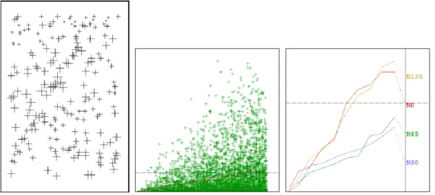
Figure 4. Data (left) – Variogram Cloud (middle) – Experimental Directional Variograms (right) ... 17

Figure 5. Experimental Variograms and Fitted Anisotropic Model ... 18

Figure 6. Estimation (left) – Standard Deviation of estimation Error (right)... 19

Figure 7. From left to right: Data Set – Punctual estimation – Block Average estimation – Gradient estimation ... 20

Figure 8. Reality (left) – Sampling (Middle) – Punctual Estimation (Right) ... 21

Figure 9. Simple variograms of both variables (top-left and bottom-right) – Cross-variogram (bottom-left) ... 21

Figure 10 Estimation maps: Kriging (left) and Co-Kriging (right) ... 22

Figure 11. Yeu Island ... 23

Figure 12. Kriging estimate with data along bathymetric profiles ... 23

Figure 13. Some simulation outcomes ... 24

Figure 14. Risk Curve for Surfaces of Yeu Island ... 24

Figure 15. Probability map of the island ... 25

Figure 16. Base map of the whole IMR dataset – Temperature (°C) at 20m depth ... 29

Figure 17. Sample selection – Temperature (°C) for first trimester of 1995 at 20m depth ... 30

Figure 18. Temperature (°C) function of depth (m) ... 30

Figure 19. Histogram of sampling depths before (left) and after (right) aggregation ... 31

Figure 20. Statistics per year at 25m depth – Mean (left) and Variance (right) of Temperature (°C) .. 31

Figure 21. Cell (i.e. block) average for Temperature at 25m depth (1995) ... 32

Figure 22. Temperature variography at 25m depth (2008 2nd trimester) ... 33

Figure 23. Temperature (°C) estimation at 25m depth (2008 2nd trimester) ... 34

Figure 24. RGeostats and RIntaros Conda packages repositories ... 36

(9)

Deliverable 5.6

Figure 26. Application design based on remote data access and Cloud-based Jupyter Notebooks ... 38

Figure 27. Elaboration of unitary data processing jobs ... 39

Figure 28. estimate.R script using RIntaros functions ... 41

Figure 29. JupyterLab workspace provided by the Ellip Notebooks solution ... 42

Figure 30. Use of Jupyter Notebooks (IMR Case Study) ... 44

Figure 31. Workflow integration and design of parallelization nodes ... 44

Figure 32. Workflow input parameters and application run (Ellip VM - test client view) ... 45

Figure 33. Application run for generation of test results (Ellip VM – console view) ... 46

Figure 34. Aggregation of filenames per output type and tile index (here tile 7 shown) ... 48

Figure 35. Metadata properties defined for a job processing output ... 49

Figure 36. Legend scales and rendering for a job processing output ... 49

Figure 37. Geobrowser with access to the application as-a-service, and visualization of processing job results ... 51

(10)

Deliverable 5.6

1 Introduction

1.1 Benefits of Geostatistics for INTAROS

Geostatistics is a branch of statistics focusing on spatial or spatiotemporal datasets. Developed originally for the mining industry, it is currently applied in diverse disciplines including geography, hydrology, meteorology, oceanography and any discipline regarding environmental control. Its main goal is to analyze the spatial characteristics of the variable of interest (its continuity, regularity, ...) and capitalize on this spatial model when interpolating this variable, from a few measured samples to a much larger zone of interest. A complementary approach is to use the same spatial model to predict all the possible variability of the variable in order to establish probability maps or risk curves.

The main geostatistical algorithms are now familiar to any earth scientist and have been incorporated in many places, including geographic information systems (GIS) and on many platforms such as INTAROS.

Here are some examples among thousands of geostatistics applications than can benefits to INTAROS partners and users community:

 Interpolation of ocean temperature or salinity fields for a given depth and time interval (from scattered data) in order to validate climate model projection,

 Filtering of the measurement error of buoys or other in-situ sensors,

 Calculation of the probability of exceeding a given sea ice thickness threshold (useful for example for planning icebreaker cruises),

 Conditional simulations of snow precipitation and resulting snow depth in order to assess the risk of avalanche,

 Filtering of the masking effect of clouds on satellite image,  Evolution of fish stocks in time and space,

 Seasonal plankton concentration analysis,

 Estimation of the repartition of white bears from in-situ observation…

Some previous real environmental case studies performed by the Geostatistical group of MINES ParisTech are described in the Section 2.6.

1.2 User driven definition of the RIntaros Geostatistical Library

INTAROS uses a widely adopted technique from software engineering to capture user needs: User stories. This technique allows us to quickly identify user needs through simple statements. The user stories are then elaborated in dialogue with users to understand their real needs and thereby enable software developers to implement a satisfactory solution.

(11)

Deliverable 5.6

One of the INTAROS user stories defined in the WP5 Deliverable 5.4 (iAOS portal user manual V1) is the following:

Processing Service #3: Generation of ocean temperature and salinity fields for validation of

climate model projections

The aim of this processing service is to enable users to apply geostatistical methods in order to interpolate scattered in situ observations of ocean temperatures into a gridded field. These interpolation maps are then useful to validate forecasts from climate models.

One of these models, the Norwegian Climate Prediction (NorCMP) model (Counillon et al., 2014) funded by the European Union (EU) and the Research Council of Norway (NFR), aims at providing climate prediction from seasonal-to-decadal time scale.

The need to compare outputs of NorCMP model with in situ observations has been defined in WP6 Task 6.3 (“Ice-ocean statistics for decisions support and risk assessment”). The requirements from this stakeholder are the following:

 Area of interest: 50°N-80°N, 30°W-60°E (North Atlantic Current, Norwegian Current, Barents Sea)

 Interpolated map resolution of 1.0 degree (regular grid)  Interpolation monthly averaged

 Ocean temperature and salinity analysis

 Additional tools or constraints required by the stakeholder have been proposed:  Retrieve the number of samples per output grid cell

 Get the statistics for a given period or a given depth

 Average the samples values for a given period or a given depth  Manipulate projections and propose some display smart features  Realize the estimation by layer near the water surface

Geostatistical methodology is a major scientific topic addressed by the Geosciences center – a common research center of ARMINES and MINES ParisTech. A large part of geostatistical methods are currently implemented in the RGeostats package (developed by the Geosciences center) and which is freely available to the scientific community (see Section 2).

Moreover ocean temperature and salinity observations in the area of interest are available in datasets from the Norwegian Marine Data Centre (NMDC) at the Institute of Marine Research (IMR) (see Section 3).

The idea for the first version of the Geostatistical Library for iAOS is to wrap geostatistical methods from the RGeostats package (data analysis, statistics, variography and kriging) and demonstrate how to use them on the observations coming from IMR dataset.

(12)

Deliverable 5.6

1.3 The Geostatistical Library

The RIntaros Geostatistical Library for iAOS aims at bringing additional knowledge, analysis and understanding to the data available in the INTAROS project. The idea is to make geostatistical methods available to the iAOS portal users as well as to the iAOS software developer community. The example below illustrates how a user can display the data of an INTAROS dataset through the iAOS Cloud Platform Geobrowser tool. In addition, the user can also invoke the Web Processing Service (WPS) named “EWF-IMR-ESTIM” in order to evaluate and display interpolated maps calculated from the same dataset.

Figure 1. Generic flow chart from data provider to user in the iAOS Cloud Platform – Example of “EWF-IMR-ESTIM” WPS Additionally to all geostatistical features coming with RGeostats package (see Section 2.2.2), the first version of the RIntaros Geostatistical Library (GL) brings the following high level features dedicated to CTD data (vertical profiles):

 Load, validate and aggregate data samples,

 extract sub-parts of the data by location, depth or time interval,

 display data samples in enhanced 2D views for a given location, depth or time interval  calculate statistics globally or for each cell of a coarse 2D grid,

 perform explanatory data analysis of interest variables by calculating the covariance model using the automatic fitting of the experimental variograms,

 interpolate (kriging) and display 2D or 3D gridded fields of interest variables at a given depth and time interval,

 check the quality of the interpolation by performing the cross validation procedure. Thus, the GL can be seen as a “wrapper” of RGeostats functions made available for particular treatments of INTAROS datasets. This means that the GL simplify the access and the use of the underlying Rgeostats package for the INTAROS partners and users community.

(13)

Deliverable 5.6

As a preliminary work performed within the INTAROS WP5, the Rintaros and the Rgeostats packages have been integrated and delivered as a Freeware packages, available to the developers’ community in charge of designing new iAOS Processing Services (see Section 4.1). 1.4 Using the Geostatistical Library in a Cloud Processing Service

In the framework of the INTAROS Task 5.4 (“Development of geostatistical methods for data integration”), a case study of the IMR dataset has been conducted using the first version of the GL (see Section 3). A new iAOS Processing Service using this new GL has been designed in order to generate interpolation and estimation error maps of the variables measured by IMR (see Section 4).

This document describes first the main possibilities offered by Geostatistics through the use of Rgeostats package. It gives an overview of the techniques that could be offered to the users of the iAOS platform.

Then, the IMR case study is briefly presented in order to demonstrate how the GL can be used for analyzing temporal and spatial data measured along vertical profiles in the North Sea.

Finally, the first Demonstrator (v1) of the iAOS application designed for generating estimation maps of IMR dataset variables (Stakeholder requirement §1.1) is described. The application is delivered to the iAOS community as-a-Service (accessed via an OGC WPS standard interface). A data processing workflow has been integrated and deployed using the Ellip Solutions available on

Terradue Cloud Platform, in order to make it available online to the iAOS portal users, and its

source code is shared as well as to software developers in charge of developing other iAOS Processing Services based on the GL.

1.5 Organisation of this report

The remainder of this document is organized as follows. Section 2 gives an overview of the geostatistical methods that are offered to users of the iAOS Cloud Platform through this library. Section 3 then briefly presents the IMR case study, the data that have been used and the initial investigation and analysis of these data. Next, Section 4 presents the design and implementation of an initial application, named EWF-IMR-ESTIM, in the iAOS Cloud Platform, powered by Terradue’s Ellip Solutions. EWF-IMR-ESTIM applies Rintaros to the IMR dataset and provides a demonstrator of new data processing capabilities for the iAOS Cloud Platform. The application offers a standard interoperability interface named Web Processing Service (WPS), enabling portals and other software clients to use it. The report concludes with a summary of achievements made in developing the Geostatistical Library for INTAROS and integrating it in the iAOS Cloud Platform, and outlines the plan for future development within the project.

(14)

Deliverable 5.6

2 Geostatistics - an overview

2.1 Generalities about Geostatistics

Geostatistics is a rather recent scientific discipline, which stands as a branch of statistics applied to spatial or spatiotemporal data. Originally developed for tackling problems in Mining Industry, it rapidly enlarged towards many other domains of application, such as Petroleum Industry, Hydrogeology, Meteorology, Climatology and Environmental Control.

The geostatistical techniques are applied on (almost) any type of data, usually called variable, as long as they are defined in a space of any dimension (possibly including time): i.e. a regionalized

variable. The information is provided as a set of data measurements: this data set can contain

only few samples or large quantities of samples. Each sample provides the value of the variables of interest, measured at a given location or time, and on a given volume (measurement support). The geostatistical procedures usually apply to a target variable. Most of them can be extended to the case of several variables, benefiting from samples measured on all these variables (the count of samples per variable can be different, i.e. heterotopic case) and from the joint spatial characteristics between these variables. This multivariate concept can even be extended further when one of the variables is measured exhaustively and can serve as a shape factor for the others (external drift method).

Geostatistics covers a whole set of produces such as:

● Modeling: capability of describing a physical phenomenon and its spatial characteristics. ● Interpolation: extending the knowledge to a whole field starting from a small set of

measurements. This corresponds to the traditional mapping concept.

● Estimation: predicting the variable contents (grade for example) in an extraction volume (mining selective unit) from samples collected on much smaller support (core samples). ● Risk analysis: predicting the probability that the field of interest exceeds a given

threshold.

Geostatistics has gained momentum and can now be found in many commercial software offers. The most well-known is certainly ISATIS©_{commercialized by}_Geovariances_{. Some functions can}

be found on Internet here and there, which perform some of the tasks mentioned above.

Another software named RGeostats is freely available on the web. It has been developed since 2001 by the Geosciences center – a common research center of ARMINES and MINES-ParisTech.

(15)

Deliverable 5.6

2.2 RGeostats Package

2.2.1 What is RGeostats?

RGeostats stands as the largest collection of geostatistical functions available within a single R

package. It can be downloaded for free from http://cg.ensmp.fr/rgeostats. Once installed in the local R environment, the user can then establish some R scripts which call RGeostats functions for a specific activity (Data analysis, Modeling, Estimation, etc…).

RGeostats is an R package which relies on a C/C++ library called Geoslib. The interface between RGeostats R functions and the C/C++ code is made possible by the Rcpp package.

Figure 2. RGeostats R package architecture

The RGeostats website proposes several services that can guide the non-expert users: demonstration scripts in a particular context (vignettes), online help for more than 500 functions available, discussion forum for troubleshooting and News. The RGeostats user community (academic and researchers) has more than 700 members in the world.

The RGeostats package and guidance for the downloading or the loading from RStudio of the R Package archive file is provided on the RGeostats website.

(16)

Deliverable 5.6

Figure 3. RGeostats website

As part of the INTAROS WP5 activities, the RGeostats software package has been made available on standard online repositories (on anaconda.org) for use on Cloud Computing environments such as defined for iAOS (cf. D5.5 - iAOS requirements and architecture consolidation V2). Please look at the §4.1 for more details.

2.2.2 RGeostats features

RGeostats (and the R platform in general) proposes a large number of statistical tools that allows the user to perform a sound analysis of its data. When the data are structured spatially (in space and/or in time), geostatistics are then useful.

This package is the basis of the contribution of ARMINES to INTAROS project. It contains all the general purpose geostatistical functionalities (developed for any space dimension), among which those requested by the project.

They can be grossly subdivided into several themes:

 The functions which are used to handle the geostatistical objects, such as the: o The normal score transformation of the distribution of the target variable (or

(17)

Deliverable 5.6

o The (numerical) Data Base where all the input and results are stored. This Data Base can be organized as a grid or simply a set of isolated points (possibly organized along lines).

o The particular Data Base for storing a network of fractures (connected or not) o The meshing or a 2-D or 3-D space (i.e. triangulation or tetrahedrization)

o The (geostatistical) Model which describes the spatial characteristics of the target (set of) variable(s)

o The Neighborhood parameters which describe the set of samples to be

considered for conditioning estimations and/or simulations: it can vary from a dozens of close samples (moving) to the whole data set (unique).

o The Polygon which delineates the area of interest where the estimation and/or simulation must be performed

o The lithotype rule which defines the vicinity relationship between classes of a categorical variable

o The experimental covariance or variogram derived from the values at samples and which give an experimental point of view on the spatial characteristics of the (set of) variable(s) of interest.

 The functions used to follow the main steps of a geostatistical workflow: o Data exploration:

Calculation of basic statistics (reporting, histogram, correlations…) Detection of possible trends

Possible data transformation (Declustering, Normal score …) o Modeling the spatial characteristics:

Computing the experimental quantities (variogram, covariance…) for a single or a set of target variables

Fitting an authorized model

o Estimation of the (set of) variable(s) on a set of targets:

Several traditional interpolation algorithm (used for comparison): inverse distance, voronoï tessellation, trend surface…)

Estimation by minimizing the estimation variance of any linear transformation of the target variable: Kriging (punctual, block average, over a territory)

Enhanced:

 in the case of multiple target variables: CoKriging

 in the case of trends (Universal Kriging) or similarities with explanatory variables (External Drift)

o Simulations:

This corresponds to a large spectrum of features depending on the type of the target variable(s). For example, let us mention, among others:

 Turning Bands or Spectral methods for continuous Gaussian variables  Boolean technique for object based simulation

(18)

Deliverable 5.6

 SPDE: for simulating random fields which obey to partial derivative equations

 PluriGaussian for simulating a categorical variable 2.3 Data Spatial Structure

All geostatistical techniques rely on the analysis of the spatial behavior of the target variable(s). These characteristics are measured experimentally from the information carried by the samples. Several statistical tools can be considered: the most basic one is the covariance (centered or not); the most well-known in the geostatistical community is the variogram; but we can also name the

variogram of increments (in the case of a non-stationary variable) or other tools such as the madogram, the rodogram, ...

This experimental quantity is then summarized in the spatial Model, which is a parametric formulation, which depends on a limited number of parameters.

2.3.1 Experimental Quantity

In this paragraph, only the experimental variogram is described. First the variogram cloud is established where all pair of data points are compared (up to a given maximum distance equal to one third of the total field extension). Each pair is represented by the variability as a function of the distance between the two samples. The variability is obtained as follows: 1₂(𝑍₁− 𝑍₂)2_where

𝑍₁ stands for the value of the target variable at the first point while 𝑍2 is the value at the second

point. Finally, the variability of these pairs is averaged by classes of distance, in order to obtain the experimental variogram. They can also be averaged by classes of direction, in order to depict some possible anisotropy.

(19)

Deliverable 5.6

This being considered as a simple example, the exact data point coordinates or the exact values of the variances are not necessary for the understanding.

The left part is a base map (data point location) where the horizontal axis covers 1km and the vertical axis 1.5km.

The middle picture is a variogram cloud describing the 2-D point statistics. As recommended in literature, the horizontal axis (distance) covers one third of the field extension. The vertical axis gives (half of) the maximum variability of a pair of points. The experimental variance of the dataset is represented as a dashed line sitting close to the bottom of the graph.

The right picture is a variogram calculated in four main directions (i.e. N0, N45, N90 and N135). The horizontal axis is the same as for the variogram cloud. The vertical axis covers the maximum variogram value (reached in directions N135 and N0). The dashed line corresponds again to the experimental variance of the data.

2.3.2 Fitting a Model

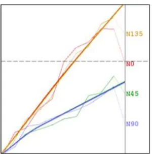
The experimental variogram calculated for several classes of distance and orientation must then be fitted by a parametric function called the Model. This function must have some nice mathematical properties (definite positiveness), which ensure that it can be used for variance calculation (always producing positive results).

Figure 5. Experimental Variograms and Fitted Anisotropic Model

2.4 Estimation

When the spatial characteristics of the variable of interest have been captured in the Model, we can envisage addressing the estimation / interpolation task performed in the Geostatistical

(20)

Deliverable 5.6

framework. The method named Kriging can be used in order to predict the variable in any target location throughout the field, starting from few measurement points. The targets can be a set of locations of interest or, more generally, the nodes of a regular grid used for mapping.

Kriging presents several virtues:

● It is unbiased: it does not present any tendency to under-estimate or over-estimate. ● It is optimal: on average, it minimizes the error that inevitably occurs in the prediction

(according to the spatial characteristics provided by the Model).

● It is an exact interpolator: the result coincides with the measured value when target and data measurement coincide.

As a by-product, Kriging also provides an evaluation of the variance of the error committed in this prediction at each target site. We usually prefer using its square root (the standard deviation), which is expressed in the same unit as the variable itself.

Figure 6. Estimation (left) – Standard Deviation of estimation Error (right)

2.4.1 Definition of the Neighborhood

The estimation procedure is obtained by solving a linear algebraic system. Its dimension is equal to the number of samples. Therefore in the case of large data set, this may become intractable. Instead the estimation for each target site can be performed using only a subset of the data located close to this target: this refers to the Moving Neighborhood concept.

(21)

Deliverable 5.6

When the data set is not too large, we may prefer using the Unique Neighborhood (where all samples are used for each target site), which offers some nice algebraic properties enabling fast processing.

2.4.2 Different Types of Estimations

We must also mention that the Kriging estimation procedure can be used in many different circumstances. The one described above corresponds to the prediction of the variable in a set of target sites (e.g. the nodes of a regular grid): it refers to the punctual estimation. This technique can be enhanced with the block average estimation used, for example, to predict the average grade over each selective mining unit (the volume unit during the exploitation) and decide if it must be sent to the mill or to the waste. Kriging can also be used to calculate gradients: this makes sense when predicting the gradient of pressure (wind) starting from atmospheric pressure measured at gauges.

Figure 7. From left to right: Data Set – Punctual estimation – Block Average estimation – Gradient estimation More generally, Kriging procedure can estimate any quantity linearly related to the measured variable. Finally Kriging can produce the global estimation for instance for estimating the total abundance of a fish species in a given portion of ocean for example.

2.4.3 Estimation Properties

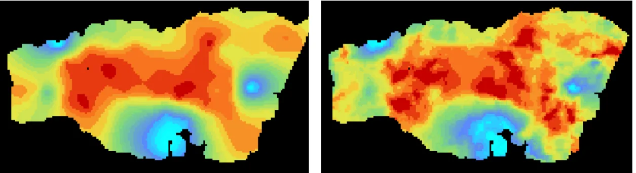
As mentioned earlier, Kriging (like any estimation based upon some optimality criterion) tends to produce estimates than are smoother than reality. This is what is demonstrated next by first producing an exhaustive data set in a field (considered as the reality), then sampling it and finally estimating it back on the field again.

(22)

Deliverable 5.6

Figure 8. Reality (left) – Sampling (Middle) – Punctual Estimation (Right)

2.4.4 Enhancement in Presence of Several Variables

The information on the variable of interest can sometimes be improved by the knowledge of an additional co-variable. The impact of this multivariate approach is measured in the Model, which reflects the joint spatial characteristics of all variables: this requires the calculation of the experimental simple variograms (of each variable considered separately) as well as the cross-variogram (of the pair of variables) that are all fitted by a multivariate Model.

Figure 9. Simple variograms of both variables (top-left and bottom-right) – Cross-variogram (bottom-left)

The estimation is then performed by a Co-Kriging procedure, which takes information from both variables into account through the multivariate Model. In the next example, we can measure the difference between the estimation of the target variable by Kriging compared to the Co-Kriging

(23)

Deliverable 5.6

result using one secondary co-variable. The Co-Kriging procedure can be extended to any number of variables treated jointly as long as they present some significant spatial correlation (at least one cross-variogram between a pair of variables is not flat).

Figure 10 Estimation maps: Kriging (left) and Co-Kriging (right)

2.4.5 External Drift Concept

We may sometime consider that the target variable, only measured at a limited number of data points, is correlated with a co-variable which is known exhaustively. Then the co-variable is used more extensively and provides the shape factor to the variable of interest: this technique is known as the Kriging with External Drift.

2.5 Simulations

Given the set of measurements of the variable of interest and its associated Model, we recall that Kriging produces two results: the estimation on one hand and the standard deviation of estimation error on the other hand. At each target site, the first one gives the most probable value (given the data and the Model) whereas the second one provides the range of plausible values for reality. Nevertheless, this information is not sufficient for global (non-linear) criteria such as the probability that a pollutant concentration exceeds a given threshold for example. For such problems, we are not looking for optimality anymore (which leads to results which are systematically too smooth to be compared to reality). Instead we wish to produce outcomes which have the same spatial behavior as reality. This refers to another technique called

geostatistical simulations which produce a series of equiprobable maps, each one of them

reproducing the input Model and honoring the data.

2.5.1 Several Realizations

The principle of the Simulations is to produce a large series of outcomes and to perform the calculation separately on each one of them. As all outcomes have the same likelihood, all the resulting values are equally possible.

(24)

Deliverable 5.6

The following demonstrative example has been carried on based on the Yeu Island (western coast of France). 40 measurements provide the elevation of the sea floor along 8 bathymetric profiles. Note that all elevations are negative (below sea level). The problem is to guess the presence of a possible island and its possible surface. The true island measures 23.32km2_.

Figure 11. Yeu Island

The first attempt is to estimate the elevation using Kriging retaining the positive results as the island: as expected the result is biased and the estimated island tends to have a too small surface (22.94km2_).

Figure 12. Kriging estimate with data along bathymetric profiles

Instead we perform a large set of simulations (some of them are represented here) and derive the surface for each outcome.

(25)

Deliverable 5.6

Figure 13. Some simulation outcomes

2.5.2 Risk Curve and Probabilities

The results are finally represented as risk curve, which gives the range of possible surfaces: the average value of these surfaces is 23.17km2_.

(26)

Deliverable 5.6

These simulation outcomes can also be exploited in order to provide, at each target point, the probability that it belongs to the island.

Figure 15. Probability map of the island

2.6 Some previous use of Geostatistics in INTAROS application fields

2.6.1 Use cases and articles

Here are some previous use cases and associated publications of the Geostatistical group from the Ecole des Mines de Paris in the INTAROS application fields.

In several domains of the geosciences (e.g., geodesy, paleomagnetism, climatology, and oceanology), data are supported by spheres. In the following paper, a new innovative technique is proposed for applying geostatistical methods on spheres:

Christian Lantuéjoul, Xavier Freulon, Didier Renard. Spectral Simulation of Isotropic Gaussian Random Fields on a Sphere, Mathematical Geosciences, Springer Verlag, 2019, 51 (8), pp.999-1020. (10.1007/s11004-019-09799-4)

The next paper presents a novel application of the geostatistical multivariate method known as min–max autocorrelation factors (MAFs) for analysing fisheries survey data in a space–time context. The method was used to map essential fish habitats and evaluate the variability in time of their occupancy:

Pierre Petitgas, Didier Renard, Nicolas Desassis, Martin Huret, Jean-Baptiste Romagnan et al. Analysing Temporal Variability in Spatial Distributions Using Min–Max Autocorrelation Factors: Sardine Eggs in the Bay of Biscay,

Mathematical Geosciences, Springer Verlag, 2020, (10.1007/s11004-019-09845-1)

The next paper present a first implementation of a particle filter into a hydro-biogeochemical model for metabolism's parameter estimation. The assimilation of a 15-min “observation”

(27)

Deliverable 5.6

dissolved oxygen data has been realized in the Seine River system on a synthetic case study: Shuaitao Wang, Nicolas Flipo, Thomas Romary (2019),

Oxygen data assimilation for estimating micro-organism communities’ parameters in river systems,

Water Research, Volume 165, 2019, 115021, ISSN 0043-1354,

https://doi.org/10.1016/j.watres.2019.115021.

In the next paper, we proposed a methodology to optimize sampling schemes of static sensors networks. This methodology is based on the construction of a relevant objective function and its optimization. Although it has been developed for air quality problems, it is general and can be adapted and applied to various natural Arctic phenomena:

Romary, T., Malherbe, L., & De Fouquet, C. (2014).

Optimal spatial design for air quality measurement surveys. Environmetrics, 25(1), 16-28.

The next paper shows how geostatistical non-linear indicator tools can be used to define hotspots in fisheries ecology as well as how inter-annual variability can be handled with multivariate geostatistics. Variograms and cross-variograms of indicators were used to estimate transition probabilities, which allowed to define hotspots in relative terms as the areas within which higher values occurred unpredictably:

Petitgas P, Woillez M, Doray M, Rivoirard J (2016)

A Geostatistical Definition of Hotspots for Fish Spatial Distributions. Mathematical Geosciences, Springer Verlag

2.6.2 Handbook for fisheries and marine ecology

Several studies have been made for fisheries and marine ecology using geostatistics through the use of RGeostats package. A handbook has been published (2017) for helping scientists in using geostatistics methodologies for these application fields:

Petitgas, P., Woillez, M., Rivoirard, J., Renard, D., and Bez, N. 2017. Handbook of geo-statistics in R for fisheries and marine ecology. ICES Cooperative Research Report No. 338. 177 pp

Download here: https://archimer.ifremer.fr/doc/00585/69732/67621.pdf

Demersal surveys are typical case of sampling schemes without preferential directions. They usually follow a stratified random sampling protocol so that samples are uniformly distributed in each large stratum. A specific variogram calculation is used.

In acoustic surveys, the sampling has usually high resolution data along parallel and regularly spaced transects (ship’s sailing tracks separated by tens of nautical miles). Variograms have been computed along and across transects with different lag distances to check for structural anisotropy in the fish distribution. The (global) estimation of population abundance can be performed in one dimension. It suffices to sum fish concentrations along the transect lines and

(28)

Deliverable 5.6

work on the one-dimensional dataset made of fish biomass per transect (Petitgas, 1993a). This technique has been applied successfully on anchovy surveys (Engraulis encrasicolus) in the Bay of Biscay.

Transitive covariograms have been computed for studying the cephalopod concentrations in 2D. Cephalopod surveys used were carrying by INRH (Institut National de Recherche Halieutique) – Casablanca – Morocco (Faraj and Bez, 2007). The data corresponds to a regular stratified sampling where one sample was taken at random in each square of a 11 x 11 nautical mile regular grid. The estimation variance of the mean over a domain V has been used for analyzing the concentration of herring (Clupea harengus) eggs over a spawning bed. The survey design is made of dredge hauls dispersed more or less evenly over the spawning bed. Kriging estimation for mapping has been considered with different neighborhood configurations. Two criteria have been studied: the weight of the mean, and the decrease in kriging weights with distance from the target point to be kriged. Multivariate geostatistics which permits studying the relationships between different regionalized variables has been used on herring mean length and bottom depth collected at the same (trawl) stations around the Shetland.

(29)

Deliverable 5.6

3 IMR Case Study

In this section, the use of geostatistical methods like the variography and the estimation is demonstrated on a particular dataset provided by the Institute of Marine Research (IMR) center of Norway.

The complete case study (report and scripts) is available in the following datasets: HTML report of the case study:

http://rgeostats.free.fr/doc/Files/imr_case_study.html

CSV of selected dataset records for the case study:

http://rgeostats.free.fr/doc/Files/imr_data_0_to_100m.csv

This case study has been used as base material for the RGeostats Workshop during the INTAROS second year General Assembly (Bremen, January 2019).

3.1 IMR Dataset Presentation

3.1.1 Global dataset volume

From 1995 to 2006, the Institute of Marine Research (IMR) center of Norway has measured the temperature, the salinity and the conductivity in the North Sea. The samples are collected along vertical profiles by 7 research vessels. After processing and quality control, these data are usually binned to one value every 1 meter depth..

Data are stored in NetCDF files (one file by year and per vessel). Coordinates are in degrees (Long/Lat) and the timestamp is the number of minutes since the 1st_{January 1950. The time frame}

of the whole dataset lies between 7th_{January 1995 and 29}th_{November 2016. There are 5.5 billion}

of samples measured over 63 500 positions (vertical profiles). The whole dataset volume is 880 GB.

All files are freely available on an OpenDAP server:

http://opendap1.nodc.no/opendap/physics/point/yearly/contents.html

Here is a base map of all the samples for the Temperature variable at 20m depth (the output estimation grid (1 degree mesh) is displayed in the background in light gray):

(30)

Deliverable 5.6

Figure 16. Base map of the whole IMR dataset – Temperature (°C) at 20m depth

3.1.2 Data selection

Each sample has a 2D coordinate (Longitude and Latitude of the vessel position), a vertical depth (along the profile) and a time stamp (date of the measure). So the data are 4D (3D + time). A first procedure named apply_sel aims at filtering the database according the:

Longitude (min and max) Latitude (min and max) Depth (min and max) Date (min and max)

In the next figure, a selection has been performed in order to outline the only measurements collected during the first trimester of 1995 at 20m depth.

(31)

Deliverable 5.6

Figure 17. Sample selection – Temperature (°C) for first trimester of 1995 at 20m depth

On the whole data set, we establish the chart representing the temperature as a function of the depth. Note that no selection has been performed on the longitude / latitude of the measurements. This global comparison proves that the temperature is decreasing with depth on average but not on a linear manner.

(32)

Deliverable 5.6

The vertical axis in the previous figure has been cut at 10°C in order to better see the curve. 3.2 Statistics Analysis

At each location, the samples are measured vertically at 1m interval. In order to provide a more representative data set, an aggregated value is obtained by averaging the values over 10m intervals. The histograms of sampling depths are provided in the next figure.

Figure 19. Histogram of sampling depths before (left) and after (right) aggregation

We can see in the left histogram of Figure 19 that there is more data every 5m depth. It means that CTD data from some vessels have been binned to every 5m instead of every 1m.

For the rest of this study, we concentrate on data obtained at 25m depth (Figure 20). For both data sets (initial and aggregated) it is interesting to examine the variability of the temperature averaged per year. We can also provide the variance attached to each value. But there is no guarantee that the investigation area is similar between years; therefore the low average (around 2013) may not be significant. The point colors in Figure 20 are for improved visual appearance.

Figure 20. Statistics per year at 25m depth – Mean (left) and Variance (right) of Temperature (°C) Another feature (prior to estimation) is simply to calculate the average of the temperature values over the cells of a regular grid (1 degree mesh). This calculation is limited to the samples

(33)

Deliverable 5.6

collected in 1995. This display clearly shows that the latitude has an higher impact on the temperature than the distance to the coast.

(34)

Deliverable 5.6

3.3 Temperature Variography and Estimation

The next step consists in analyzing the spatial characteristic of the temperature. As we concentrate on the data collected at 25m depth, the temperature is considered as a 2D variable. Therefore it suffices to calculate the 2D variogram. Moreover, and for sake of simplicity, only the omni-directional has been investigated (assuming that there is no influence of the direction on the spatial variability). The experimental variogram is (automatically) fitted to a Model.

The fitted Model (see next Figure) contains an important proportion of Nugget Effect (small scale variability), a structure extending to two degrees and a linear component for large scale.

Figure 22. Temperature variography at 25m depth (2008 2nd_trimester)

Vertical axis covers the variogram values calculated in all direction (omni-directional variogram) When the Model has been determined, we can perform the estimation at the nodes of the regular grid. Note that the estimation area has been reduced around the southern part of Norway in order to avoid too much extrapolation.

(35)

Deliverable 5.6

(36)

Deliverable 5.6

4 IMR Estimation Application Workflow (WPS)

4.1 RIntaros and RGeostats

In order to simplify the use of the RGeostats package and improve the accessibility to geostatistical methods for the INTAROS community, a Geostatistical Library has been created. It is a new R package named RIntaros, which relies on RGeostats. The first version or RIntaros is dedicated to IMR dataset.

The general description of the features of RGeostats is done in §2.2.2. Those for RIntaros are described below for comparison.

The RIntaros package has been explicitly develop to complement RGeostats when manipulating spatial data coming from IMR Data Base or for packaging sets of specific workflow to reduce their complexity for non-expert users. We can distinguish:

 Utilities for processing IMR data (reading according to specific formats, date conversion, selection based on time or depth intervals)

 Specific workflows for:

o Basic statistics benefiting for spatial coarse gridding or analysis of time series o Modeling the spatial structure of target variable(s)

o Estimation in 2-D (by vertical layers for example) or in 3-D o Blind test or Cross-validation

RGeostats and RIntaros software packages have been made available on standard online repositories (on anaconda.org) for use on Cloud Computing environments such as defined for

iAOS (cf. D5.5 - iAOS requirements and architecture consolidation V2).

Evolutions of the RGeostats and RIntaros software are being maintained by ARMINES and regularly updated on the following online repositories for the convenience of INTAROS partners developing new iAOS Processing Services:

● Repository of latest Conda package build for RGeostats:

https://anaconda.org/Terradue/r-rgeostats

e.g. r-rgeostats 11.2.11, uploaded on 2019/10/16 ● The related build recipe is documented here:

https://github.com/ec-intaros/r-rgeostats

(37)

Deliverable 5.6

● Repository of latest Conda package build for RIntaros:

https://anaconda.org/Terradue/r-rintaros e.g. r-rintaros 1.7, uploaded on 2019/11/26 ● The related build recipe is documented here:

https://github.com/ec-intaros/r-rintaros

Figure 24. RGeostats and RIntaros Conda packages repositories

r-rgeostats and r-rintaros anaconda packages are available for the INTAROS community to be freely downloaded from their repositories since September 2019.

Their adoption by the INTAROS community is being promoted through the joint work of WP5 and WP6 on the development of showcase applications for the iAOS.

4.2 Using the Ellip Solutions to build new iAOS Processing Services

The Ellip Solutions, provided by the INTAROS Partner Terradue as part of the iAOS environment, enable subscribers to work with a Platform-as-a-Service environment, providing them with an integrated user experience for the design and test of their data processing unitary functions (including for sharing towards partners as a reproducible experiments), for the design, integration and test of scalable processing chains, for the packaging and deployment of validated processing services on Production servers from a selected Cloud Provider, as well as the monitoring of the execution and result generation of the deployed processing services.

The Ellip Dashboard provides an integrated online access to the different services, and from there, a typical scenario is for the user to follow the journey as depicted hereafter:

(38)

Deliverable 5.6

Figure 25. Ellip Solutions user dashboard & usage baseline scenario An overview of the Ellip solutions is provided online here:

● https://www.terradue.com/portal/ellip (core services and solutions portfolio)

● https://ellip.terradue.com (Ellip Dashboard, subscription-based access only)

● https://docs.terradue.com/ellip (online documentation)

Note 1: the Ellip Solutions have been introduced in more details within the INTAROS Deliverable

D5.5 - iAOS requirements and architecture consolidation V2

Note 2: the status as of January 2019 of the integration work is provided online here:

https://intaros.nersc.no/system/files/INTAROS%20WP5%20-%20IMR%20Dataset%20and%20RGeostats_0.pdf

(39)

Deliverable 5.6

currently on going where the Geostatistical Library is involved. Results will be available during the year 2020.

4.3 Application Design

As part of the INTAROS project, a collaboration with the project partner IMR provided the iAOS with a first online version of a data server (based on the OpenDAP standard protocol) and delivering the IMR datasets introduced in the previous section (temperature, salinity and conductivity in the North Sea).

Figure 26. Application design based on remote data access and Cloud-based Jupyter Notebooks

By accessing the Ellip Notebooks solution, a series of data processing functions have been designed and tested on a JupyterLab environment.

On this work environment, the RIntaros and RGeostats libraries have been pre-installed by ARMINES with the support of Terradue, in order to exploit the selected IMR dataset.

(40)

Deliverable 5.6

Figure 27. Elaboration of unitary data processing jobs

The scripts developed by ARMINES address the different operations of data filtering and data processing useful for exploring and analyzing dataset contents.

We provide hereafter an overview of the ‘downloadData.py’ and ‘estimate.R’ functions and their software dependencies, especially for the later onto the RIntaros and RGeostats libraries.

(41)

Deliverable 5.6

(42)

Deliverable 5.6

Figure 28. estimate.R script using RIntaros functions

A set of data management scripts resulting from this activity are available as Jupyter Notebook files (.ipynb) and are synchronized online on a public Git repository:

https://github.com/ec-intaros/RGeostats-workshop

(43)

Deliverable 5.6

Figure 29. JupyterLab workspace provided by the Ellip Notebooks solution

Once loaded, the INTAROS IMR Case study comes with Workshop material such as a Geostats Course and a description of the IMR Dataset in scope of the RGeostats Course, as well as the executable Notebook files that are embedding the data management scripts.

(44)

Deliverable 5.6

(45)

Deliverable 5.6

Figure 30. Use of Jupyter Notebooks (IMR Case Study)

4.4 Application Workflow integration and tests

From the initial design and test activities presented in the previous chapter, a next step is to integrate these functions as part of a scalable data processing service.

Here the aim is to have the resulting data processing Workflow deployed and operated as-a-Service, for example accessed online by a range of users from a dedicated iAOS Web portal.

Figure 31. Workflow integration and design of parallelization nodes

Once the data processing chain is integrated using the tools and APIs provided by the Ellip Workflows solution, it can be tested from within the ‘Sandbox’ virtual machine where it is integrated.

Application runs can be tested from the Browser (accessing the Virtual Machine through secured VPN connection).

(46)

Deliverable 5.6

(47)

Deliverable 5.6

Application runs can also be tested from the Console (accessing the Virtual Machine through secured SSH connection).

$ ciop-run

2019-10-16 16:29:06 [INFO ] - Upload results? null jar:file:/usr/lib/ciop-run/ciop-joozie-1.2.jar!/schemas/oozie-workflow-0.1.xsd

2019-10-16 16:29:06 [INFO ] - Workflow submitted

2019-10-16 16:29:06 [INFO ] - Closing this program will not stop the job. 2019-10-16 16:29:06 [INFO ] - To kill this job type:

2019-10-16 16:29:06 [INFO ] - ciop-stop 0000020-191005043900365-oozie-oozi-W 2019-10-16 16:29:06 [INFO ] - Tracking URL:

2019-10-16 16:29:06 [INFO ] -

http://sb-10-150-3-19.intaros.terradue.int:11000/oozie/?job=0000020-191005043900365-oozie-oozi-W

Node Name : node_split Status : OK

Node Name : node_download Status : OK

Node Name : node_estimate Status : OK

Node Name : node_legend Status : OK

Publishing results...

2019-10-16 16:38:29 [INFO ] - Workflow completed.

2019-10-16 16:38:29 [INFO ] - Output Metalink:

http://sb-10-150-3- 19.intaros.terradue.int:50070/webhdfs/v1/ciop/run/download_and_estimation_workflow/0000020-191005043900365-oozie-oozi-W/results.metalink?op=OPEN

(48)

Deliverable 5.6

Version 1.8 Date: 23 June 2020 page 47 4.5 Application Workflow deployment for user access

As part of the Ellip Solutions, the PaaS environment offers a capacity to:

- Deploy the processing service on production servers, where it can be run at scale on a large Cloud Computing cluster.

- Simply generate a parameterized Geobrowser application, that can be used to reference the deployment of the Processing Service, run it, monitor the data processing jobs that are interactively launched, and visualize/analyse the generated results.

The definition of the processing service output product files, metadata files and legend has to comply to a simple set of design conventions (part of the online Ellip documentation) in order to be automatically discovered and handled by the Geobrowser application.

The Geobrowser of the portal can then use the metadata of a job processing results to handle data visualization on the map. It actually exploits the Terradue Cloud Platform API for this task. For instance, the processing service output product files, metadata files and legend have to comply with the following guidance:

Files aggregation

As a first process, the dataset files are listed to find all similar files, and regroup them as a single result entry. The filename without the extension is used for this aggregation.

For the IMR Case Study, the application outputs are grouped as shown hereafter, following the convention provided by Terradue for the Ellip Workflows applications:

(49)

Deliverable 5.6

(50)

Deliverable 5.6

Data properties

A dataset shall also contain a Java properties file (key=value), named as the data file it described by replacing the extension or suffixing with .properties, to give additional information about a result file. This additional information will be added into the metadata entry of the output file as metadata information. All keywords / value from the .properties file are added as a table to the summary element (used for metadata display on the geobrowser).

For the IMR Case Study, the product metadata properties are defined as shown hereafter, following the convention provided by Terradue for the Ellip Workflows applications:

Figure 35. Metadata properties defined for a job processing output

Legend

In order to attach a legend to describe the dataset, a file suffixed with .legend.png enables a map functionality that displays the legend when the data is selected.

For the IMR Case Study, the product legends are defined based on the normalized range of values from the output products, to with a color scale is applied, as shown hereafter, following the convention provided by Terradue for the Ellip Workflows applications:

(51)

Deliverable 5.6

(52)

Deliverable 5.6

After the application release and deployment based on such implementation step in the application code, the processing service output products can then be automatically discovered and handled by the Geobrowser application, for rendering and visual exploitation by users of the service.

Figure 37. Geobrowser with access to the application as-a-service, and visualization of processing job results The Geobrowser application used as an example here is a private application provided to ARMINES on the Ellip Infohubs solution (operated by Terradue for iAOS, see D5.5 and D5.8). ARMINES can control the user sharing configuration for such a Geobrowser application.

The iAOS portal is also making use of Geobrowser-like applications, and an example of the EWF-IMR-ESTIM workflow integration on the iAOS Portal will be described in the next version of this deliverable (as indicated in Section 5). The technical solution foreseen is for the iAOS Portal developed by the coordinator NERSC to access the EWF-IMR-ESTIM processing service (deployed on the iAOS Cloud Platform) via the interoperability protocol "OGC WPS” that is natively supported by Ellip-powered processing services.

(53)

Deliverable 5.6

5 Conclusion

This deliverable presented two achievements related to the first version of the Geostatistical Library for iAOS, named RIntaros:

 a software package for R, versioned and maintained with evolutions as an extension to the RGeostats library, and accessible from its online repository for download and installation by the iAOS partners, as well as the broader user community. RGeostats and RIntaros packages are freely available from https://anaconda.org/Terradue/r-rgeostats and https://anaconda.org/Terradue/r-rintaros

 a processing service (ewf-imr-estim) providing a data interpolation application (interpolating scattered in situ observations of ocean temperature and salinity to gridded fields), based on the iAOS cloud platform APIs which empowers the application with interoperable data access mechanism (based on OpenDAP), scalable data processing capabilities (based on Hadoop MapReduce) and standard processing invocation and results retrieval (based on OGC WPS specifications), for integration with the iAOS Portal of other Geobrowser applications.

This first version of the Geostatistical Library offers high level features dedicated to CTD data (validation, aggregation, global or local statistics, variography, estimation of 2D or 3D field, 2D or 3D scatter or gridded data visualization). It was matured in collaboration with the Norwegian Institute of Marine Research (IMR), in order to meet the needs of a case study based on requirements from Task 6.3 (“Ice-ocean statistics for decisions support and risk assessment”) for comparing output from the Norwegian Climate Prediction Model (NorCPM) with in situ observations. The iAOS processing service is generating ocean temperature and salinity fields for validation of climate model projections.

As a proof of concept, the processing service ewf-imr-estim was ran from an Ellip Geobrowser application, made available to the iAOS partners as part of the iAOS cloud platform operated by Terradue.

An additional exploitation stage for the iAOS partners in WP5 will be to replicate this interoperability mechanism as part of the iAOS Portal itself.

This integration work is yet still evolving: the Ellip Solutions support the iAOS partners to manage the development of their processing services and the deployment in production of new service versions, with all the procedure and tools available for such application lifecycle management. Beyond the integration work performed using the iAOS cloud platform and tools, plans for future development include the extension of the use cases from other INTAROS partners (from WP6) so they can use RIntaros and the developed applications to showcase their use of iAOS for practical use of Arctic data in scientific applications.

(54)

Deliverable 5.6

(55)

This report is made under the project

Integrated Arctic Observation System (INTAROS)

funded by the European Commission Horizon 2020 program Grant Agreement no. 727890.