Quantification of model uncertainty in RANS simulations: A review

Science Arts & Métiers (SAM)

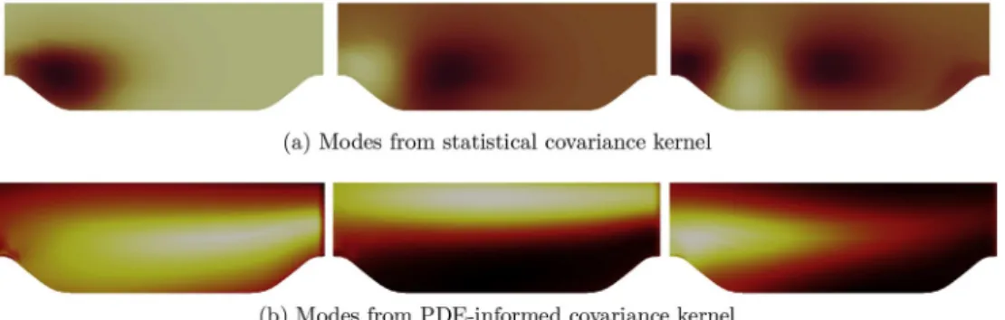
is an open access repository that collects the work of Arts et Métiers Institute of

Technology researchers and makes it freely available over the web where possible.

This is an author-deposited version published in:

https://sam.ensam.eu

Handle ID: .

http://hdl.handle.net/10985/15519

To cite this version :

Heng XIAO, Paola CINNELLA - Quantification of model uncertainty in RANS simulations: A

review - Progress in Aerospace Sciences - Vol. 108, p.1-31 - 2019

Any correspondence concerning this service should be sent to the repository

Administrator :

[email protected]

Quantification of model uncertainty in RANS simulations: A review

Heng Xiao

_{, Paola Cinnella}

a_{Kevin T. Crofton Department of Aerospace and Ocean Engineering, Virginia Tech, Blacksburg, VA, 24060, USA} b_{Laboratoire DynFluid, Arts et Métiers ParisTech, 151 Boulevard de l’Hopital, 75013, Paris, France}

A R T I C L E I N F O

Keywords:

Model-form uncertainty Turbulence modeling

Reynolds-averaged Navier–Stokes equations Bayesian inference

Machine learning

A B S T R A C T

In computational fluid dynamics simulations of industrial flows, models based on the Reynolds-averaged Navier–Stokes (RANS) equations are expected to play an important role in decades to come. However, model uncertainties are still a major obstacle for the predictive capability of RANS simulations. This review examines both the parametric and structural uncertainties in turbulence models. We review recent literature on data-free (uncertainty propagation) and data-driven (statistical inference) approaches for quantifying and reducing model uncertainties in RANS simulations. Moreover, the fundamentals of uncertainty propagation and Bayesian in-ference are introduced in the context of RANS model uncertainty quantification. Finally, the literature on un-certainties in scale-resolving simulations is briefly reviewed with particular emphasis on large eddy simulations.

A roadmap of this review article is provided above. The table of contents is also available as PDF bookmarks in the electronic version). 1. Introduction

Turbulence affects natural and engineered systems from sub-meter to planetary scales yet it is among the last unsolved problems in

classical physics. Accurate predictions of turbulent flows are of vital importance for the design, analysis, and operation of many critical systems in aerospace engineering such as aircraft, spacecraft, and gas turbine engines. The dynamics of fluid flows is described by the

∗_{Corresponding author.}

E-mail addresses:[email protected](H. Xiao),[email protected](P. Cinnella). 1_{Contributed equally.}

https://doi.org/10.1016/j.paerosci.2018.10.001

Nomenclature Symbols

ensemble averaging or spatial filtering

L2 L2 norm

A_P1 norm of A the inverseP 1 of covariance matrix P, i.e.,

A_P 1A

perturbed quantities

transpose of vectors and matrices : _{double dot of tensors} ij U_xi_j : U

Hadamard (element-wise) multiplication

Roman letters

a anisotropy tensor c1,c2,c3 barycentric coordinates

C ,1C ,2 CµRANS model coefficients

Cs Smagorinsky constant

ov covariance of random variables

d discrepancy of observation and truth

D Dt

· _{material derivative}

D data used for inference

D dissipation of turbulent frequency Z

[ ] expectation of random variable Z

f functional mapping ( , ) GP Gaussian process h unit quaternion H observation matrix i j k, , indices

I second-order identity tensor

I number of scenarios

J objective function in optimization

k turbulent kinetic energy

K ( , ) kernel for Gaussian processes

K Kalman gain matrix (in EnKF)

K number of models

l length scale in covariance kernel L linear differential operator M,Mi set of models; model

n _{axis of rotation}

N normal distribution

N nonlinear differential operator

( )

O of the order of

p instantaneous pressure p pressure fluctuation

p z( ) probability distribution of Z

P1,P2 two locations in wing–body juncture flow

(discrete) probability mass function

P production (of TKE, Reynolds stresses, or turbulent fre-quency)

P covariance matrix of state vector

P mean pressure

q mean flow features Q rotation matrix

real number space

R covariance matrix of observation error

S strain rate tensor S source terms

S˜i scenario (in BMSA)

t time

T transport of turbulent frequency ui,u instantaneous velocity

u_i, u velocity fluctuation

Ui, U mean velocity

Z

ar[ ] variance of random variable Z

V eigenvectors of second order tensor w coefficients in expansion of random field

W Wiener process (in SDEs) xi,x spatial coordinates

y model output

z augmented state vector

Z, z random variable and its realization

Greek letters

α index for basis functions

β multiplicative discrepancy field

γ parameter in regularization term

g grid spacing/filter width in LES

δ discrepancies

ij Kronecker delta, second-order identity tensor

ϵ noise in experimental data ε dissipation rate

ζ truth in the context of model uncertainty θ, model parameter(s)

ϑ angle of rotation κ von Karman constant

i eigenvalues for anisotropy tensor

diagonal matrix of eigenvalues for anisotropy tensor

μ dynamic viscosity of fluids

ν kinematic viscosity

t turbulent eddy viscosity

ξ physical state of the system ρ fluid density

latent variables (e.g., geometry, boundary conditions in CFD model)

σ variance (field) of random fields

k, coefficients in turbulence models

covariance matrix Reynolds stress

t turbulent viscosity

x

( )

i basis functions (e.g., from Karhunen–Loeve expansion) i Euler angles

quantities to be predicted

ω turbulent frequency rotation-rate tensor

Abbreviations

BMSA Bayesian model–scenario averaging CFD computational fluid dynamics DNS direct numerical simulation

EARSM explicit algebraic Reynolds stress model EnKF ensemble Kalman filtering

gPC generalized polynomial chaos LES large eddy simulation LHS Latin hypercube sampling PCE polynomial chaos expansion PDE partial differential equation pdf probability density function pmf probability mass function MAP maximum a posteriori QoI quantity of interest MLMC multilevel Monte Carlo MCMC Markov chain Monte Carlo NS Navier–Stokes

RANS Reynolds-averaged Navier–Stokes RSTE Reynolds stress transport equation

Navier–Stokes (NS) equations. While many applications in aerospace engineering involve compressible flows, reacting flows, or two-phase flows, for illustration purposes we restrict our attention to the NS equations for incompressible flows of constant-property, Newtonian fluids, shown below:

u x 0 i i = (1a) u t u u x p x Re u x x ( ) 1 _, i i j j i i j j 2 + = + (1b) whereui, p,xiand t are, respectively, the flow velocity, pressure, and

spatial and temporal coordinates. Although simpler in form than the partial differential equations governing the above-mentioned problems, incompressible NS equations cover a very wide variety of flow config-urations and bear the key difficulty that leads to the turbulence mod-eling dilemma, i.e., the nonlinear convective term in Equation (1b). Equation (1)is normalized with respect to a reference lengthLref, a

reference velocityUref, and the density ρ and viscosity μ of the fluid. The

parameter Re= U Lref ref/µis the Reynolds number, a measure of the

relative importance of inertia to viscous forces. Because of the non-linearity of the convection terms (u ui j)/ xj, the NS equations admit

chaotic solutions when the Reynolds number is beyond some flow-de-pendent critical value. As the Reynolds number increases, eventually the flow reaches a state of motion characterized by strong three-di-mensional and unsteady chaotic fluctuations of the velocity and pres-sure fields, which is referred to as the turbulent regime.

1.1. Landscape of turbulence modeling

Turbulent flows are characterized by a wide range of spatial and temporal scales. Consequently, performing direct numerical simulations (DNS) by solving the NS equations and resolving all the turbulence scales are prohibitively expensive, particularly for high Reynolds number flows. Practically used turbulence modeling strategies range from DNS with the highest fidelity, where all physics of spatial and temporal scales are resolved and no modeling is involved, to Reynolds averaged Navier–Stokes (RANS) simulations with the lowest fidelity, where the entire range of turbulent flow scales is modeled. This model hierarchy is illustrated inFig. 1, with the top represented by the most physics-resolving and computationally expensive approach (DNS) and the bottom by the most empirical and computationally affordable ap-proach (RANS). Lower fidelity models toward the bottom of the hier-archy involve more flow-dependent, uncertain closures than the higher-fidelity, scale-resolving approaches towards the top of the hierarchy. On the other hand, high-fidelity, scale-resolving models are more sus-ceptible to influences from numerical uncertainties as well as initial and boundary conditions.

A compromise between DNS and RANS simulations at two ends of the spectrum is large eddy simulation (LES), in which only the larger, more energetic scales are resolved, while scales below a cutoff threshold are filtered out. The filtered Navier–Stokes equations contain a subgrid-scale (SGS) stress that is unclosed and needs to be modeled. The SGS stress term represents the interactions between the filtered and resolved scales, which result from the nonlinear convection term [2]. Large eddy simulations have significantly reduced computational costs compared to DNS for shear flows far removed from wall boundaries. Unfortunately, they remain prohibitively expensive for wall bounded flows at high Reynolds number due to the small yet energetic scales dominating the dynamics in the near-wall regions [3]. This challenge

has led to the development of methods combining LES in free shear regions with RANS models or other simplified models (e.g., boundary layer equation or law of the wall) in the under-resolved near-wall re-gions. Such approaches include hybrid RANS/LES models [4,5] and wall-modeled LES [6–9], among others.

While scale-resolving simulations such as DNS, LES, and hybrid RANS/LES provide more insights of fluid flow physics, in many simu-lations of engineering turbulent flows such as those for aerodynamic design and optimization, the quantities of interest depend on the mean flow only, and the instantaneous flow fields are not of concern. In these cases it is desirable to solve for the mean flow more efficiently. For that purpose, the instantaneous velocityui and pressure p are decomposed

into the sum of the mean2_componentsU

iand P and the fluctuations ui

andp, respectively. Substituting the decomposition into the Navier–-Stokes equations and taking the ensemble-average leads to the RANS equations: U x 0 i i = (2a) U t U U x P x Re U x x u u x ( ) 1 _. i i j j i i j j i j j 2 + = + (2b) The RANS equations are similar in form to the Navier–Stokes equations except for the term involving the tensor u ui j. As with the SGS stress

term in the filtered NS equations for LES, this term stems from the nonlinear convection term in the NS equation and represents the cross-component covariance among the velocity fluctuations. It is often re-ferred to as Reynolds stress due to its formal similarity to the viscous stresses and is denoted as

u u .

ij= i j (3)

Since the velocity fluctuations are not available in RANS simulations, one must resort to closure models to supply Reynolds stresses, which lies at the root of most efforts of turbulence modeling.

The choice of the appropriate modeling level remains a matter of expert judgment. In particular, it inevitably involves a compromise RSTM Reynolds stress transport model

SA Spalart–Allmaras (turbulence model) SDE stochastic differential equation

SGS sub-grid scale

TKE turbulent kinetic energy UQ uncertainty quantification

Fig. 1. A schematic representation of the hierarchy of turbulence modeling

approaches based on computational costs and the amounts of resolved versus modeled physics. Figure inspired by Sagaut et al. [1]. Abbreviations: DNS, di-rect numerical simulations; LES, large eddy simulations; RANS, Reynolds-averaged Navier–Stokes.

2_{Note that several definitions exist for the mean or average quantities [see,} e.g., 10]. The most general one is the statistical ensemble average, which however is rarely used in current practice due to the large number of in-dependent flow realizations required for convergence. For statistically steady flow, time average is used instead based on an ergodicity hypothesis. The same is also used for unsteady flows, although its validity is still controversial.

between computational cost and predictive accuracy. Even after a given fidelity level is selected (e.g., RANS or LES), several possible closure models may be designed for relating the unclosed terms to the resolved variables. These closure models differ both by their mathematical structure and by the associated model parameters. The common prac-tice in turbulence modeling is to leave the choice of a specific closure model to user judgment and to treat model parameters as adjustable coefficients that are generally calibrated to reproduce simple, canonical flows. Both of the preceding aspects, however, represent sources of uncertainty in the prediction of new flows. Recent development of turbulence modeling in RANS, LES, and hybrid approaches has been reviewed by Durbin [11]. Despite considerable progress recently made in LES and hybrid RANS/LES models (e.g., [2–4,12,13]), RANS models are expected to remain the workhorse in engineering practice for dec-ades to come, due to their much lower computational costs and superior robustness. For this reason, our review mainly focuses on the quanti-fication and reduction of uncertainties in RANS models.

The landscape of RANS-based turbulence modeling has not changed for decades. The stagnation is evident from two observations as illu-strated inFig. 2. First, the number of wind tunnel tests performed in a typical design cycle of a commercial airplane was reduced from 75 in the 1970s to 10 in the 1990s, but this number has been stagnant since then, with turbulence models being the major bottleneck in predictive accuracy [14]. Second, most of the currently used turbulence models were developed decades ago and provide unsatisfactory performance for many flows. Generations of researchers have labored for many decades on dozens of turbulence models, yet none of them achieved predictive generality. Flow-specific tuning and fudge functions are still an indispensable part of RANS simulations [15]. Current development of improved turbulence models faces the dilemma of conserving the low computational costs and high robustness of RANS approaches while incorporating as much physics as possible.

1.2. Origin of uncertainties in RANS models

A recent review on data-driven turbulence modeling strategies [16]

classified the model uncertainties in RANS simulations into four levels, including uncertainties due to information loss in the Reynolds-aver-aging process, uncertainties in representing the Reynolds stress as a functional form of the mean field, uncertainties in the choice of the specific function, and uncertainties in the parameters of a given model. In this review, we will focus on the uncertainties due to the choice of functional forms and parameters in the turbulence models.Fig. 3shows a graphical representation of different sources of model uncertainties in typical RANS models.

The following observations about the Reynolds stress tensor have profound implications for turbulence modeling and RANS model un-certainty quantification. First, it is a covariance tensor of velocity fluctuations as pointed out above, and mathematically any covariance tensor must be symmetric positive semi-definite. This is referred to as

realizability requirement. Second, it appears in the RANS momentum

equation through its divergence . While the Reynolds stress as a symmetric rank-two tensor has six independent components, the di-vergence as a forcing term only has three components. The majority of existing turbulence models use the Reynolds stress as the target of modeling (Fig. 3). The rationale behind this choice is that the diver-gence form makes it easier to ensure conservation of momentum. That is, in this form the momentum is introduced into the system by the modeled Reynolds stress only through the boundaries and not within the volume. In contrast, directly constructing such a conservative for-cing term is not straightforward [17]. Therefore, in the remainder of this paper we discuss only turbulence models based on the Reynolds stress .

Reynolds stress based turbulence models require prescribing a constitutive relation for as a function of the mean flow fields. The most widely used class of models, generally known as linear eddy viscosity models, relies on the Boussinesq analogy (see, e.g., [10]). This assumption states that the anisotropic part of behaves similarly to the viscous stress tensor of a Newtonian fluid, i.e. it is a linear function of the local mean flow rate-of-strain Sij:

k _S 2 3 2 ij+ ij= t ij _(4a) S U x U x with 1 2 , ij i j j i = + (4b) where ij+2₃k ijis the Reynolds stress anisotropy, k=1₂u ui i = 1₂ iiis

the turbulent kinetic energy with a summation over index i implied, ij

is the Kronecker delta (or the second order identity tensor in its vector formI), and the eddy viscosity tis the proportionality scalar.

The limitations of the Boussinesq assumption have been widely re-cognized in the literature, particularly for flows with separation, streamline curvature, or strong pressure gradients (see, e.g., [10] for a review). Since it is often not possible to know beforehand if one or more of such flow features will be present in a new flow configuration,

Fig. 2. Stagnation of turbulence modeling in the past few decades (shaded

re-gions), showing (a) the number of wind tunnel tests required in the design cycle of commercial aircraft in the past five decades [14] and (b) the time at which commonly used models were developed.

Fig. 3. Stages of turbulence modeling in commonly used models with Reynolds stress transport models and linear eddy viscosity models as examples. Such a

hierarchy provides a clear map on where model uncertainties can be introduced and inferred (shown as shaded items).D

predictions based on the RANS equations are flawed by a structural (i.e. model-form) uncertainty [18,19]. Several attempts have been made to overcome the weaknesses of linear eddy-viscosity models, e.g., by de-veloping nonlinear eddy viscosity models [20], explicit algebraic Rey-nolds stress models (EARSM) [21], and Reynolds stress transport models (RSTM) [10,22]. All such models rely on more sophisticated constitutive relations than Equation (4). Nevertheless, such

sophisticated models lack the robustness of the simple linear eddy viscosity models. For example, cubic eddy viscosity models involve many more parameters, which are difficult to calibrate with available data [23]. As another example, the Reynolds stress transport equations have a pressure–strain-rate that needs to be modeled, and the predictive performance of RSTM are highly sensitive to its modeling. Conse-quently, the lack of robustness restricts these advanced models to a

Fig. 4. Examples of uncertainties in RANS predictions of pressure coefficient Cpdistribution on wings and airfoils due to (a) model form and (b) model coefficients.

Panel (a) shows the Cpprofile on a CRM wing-body configuration at 4. 0 angle of attack. Results are from the 6thAIAA CFD drag prediction workshop based on

different RANS models, including k–ε model, k–ω model, SA model, SA with quadratic constitutive relation (QCR), and EARSM. The location of the presented pressure distribution is indicated by the red/solid line on the wing (see inset; showing the port half of the fuselage and the wing only). Figure reprinted with permission from Tinoco et al. [24]. Panel (b) shows the Cpprofile on a NACA0012 airfoil in a transonic flow with freestream Mach number 0.8 and Reynolds number

9_×106_{, obtained from RANS simulations with the algebraic model of Baldwin and Lomax [25]. The figure shows the effect of varying Cwk, one of the seven model} parameters, from 0.25 to 1, adopted from an unpublished report of the second author [26]. (For interpretation of the references to colour in this figure legend, the reader is referred to the Web version of this article.)

Fig. 5. Roadmap of this review with links to relevant

sections. Legend: major elements of this review; auxiliary topics of this review; detailed topics in RANS model-form uncertainty.

small fraction of practical turbulent flows despite their theoretical su-periority [15], and no turbulence models are able to accurately predict the flow physics in all circumstances. The importance of model un-certainty is clearly illustrated in Fig. 4a, which shows the predicted pressure distribution on the wing section of a Common Research Model (CRM) predicted by a number of turbulence models. A large scattering of the predictions is observed, particularly downstream of the shock wave generated at the upper wing surface.

In addition to the structural uncertainties, parametric uncertainties arising from the coefficients closure models also have to be accounted for. Such coefficients are usually calibrated against experimental data for a set of simple flows (e.g., the decay of homogeneous and isotropic turbulence, flat plate boundary layers, and simple shear flows), which are generally far from practical applications. Moreover, the calibration data suffer from measurement errors, which inevitably impair the credibility of the calibrated parameters. Finally, many of the nominal coefficients found in the RANS modeling literature may not correspond to best-fit of calibration dataset, but were chosen based on numerical considerations. In practice, the closure coefficients are often empirically re-tuned by using heuristic and trial-and-error approaches in order to fit available data for a target class of flows.Fig. 4b illustrates the effect of varying only one of the seven parameters in the algebraic model of Baldwin and Lomax [25]. In particular, the location of the shock wave at the airfoil upper surface and the post-shock pressure are very sen-sitive to the varied coefficient [26].

Both the parametric and the structural uncertainties mentioned above are of epistemic nature, i.e. theoretically they could be reduced when better knowledge of turbulent flow physics and/or more abun-dant or more accurate data become available. This is in contrast to

aleatory uncertainties, which arise from intrinsic variability of a

pro-cess, e.g., uncertainties in manufactured geometries [27,28], operation conditions of turbines or aircraft [29] or inflow conditions [30,31]. In practice, reducing epistemic uncertainties by leveraging additional knowledge (e.g., by developing more advanced models to incorporate such knowledge) is far from straightforward. Additionally, sophisti-cated models may lack numerical robustness or incur excessive com-putational costs. Except for a few canonical examples, it is challenging, if not impossible, to identify the dominant source of uncertainty with definitive evidence, even for a given flow and a specific turbulence model. For instance, in many cases it is possible to improve the results of a model flawed by structural inadequacy by over-tuning its closure parameters. However, such over-tuning typically leads to poor predic-tions when applying the model to different flows from the calibration flows. Such a phenomenon is referred to as over-fitting in statistics and machine learning [32].

1.3. Approaches for quantifying uncertainties in turbulence models

Empirical assessment of uncertainties in turbulence models dates back to the early days of turbulence modeling, but rigorous treatments of such uncertainties in a statistical framework is only a recent devel-opment. While it is a consensus that aleatory uncertainties are best represented in a probabilistic framework, different approaches have been pursued for epistemic uncertainties. Because epistemic un-certainties come from lack of knowledge, it is a philosophical question whether to treat such uncertainties in probabilistic framework. In the Bayesian framework, all sources of uncertainty are represented as subjective beliefs and assigned a measure of probability. This review primarily focuses on Bayesian approaches. However, many other non-Bayesian or non-probabilistic approaches for treating epistemic un-certainties exist. Examples include imprecise probability theory [33], probability bounds analysis [34–36], Dempster–Shafer evidence theory [37], fuzzy sets [38], and credal sets [39]. For an overview and ap-plications of some of these approaches, see Refs. [40,41].

Current approaches for quantifying the model-form uncertainties associated with RANS simulations can be classified into parametric and

non-parametric approaches3_{depending on where the uncertainties are}

introduced. In parametric approaches, uncertainties are introduced to the closure coefficients of chosen turbulence models, based on which the overall prediction uncertainties are assessed. Although neglecting uncertainties in the model forms and constrained by the baseline models, the parametric approach has the advantage of being non-in-trusive and thus readily available to CFD practitioners. On the other hand, non-parametric approaches directly investigate the uncertainties on modeled terms (fields in RANS solvers), e.g., the eddy viscosity [42], source terms in the turbulent transport equations [43], or the Reynolds stress itself [44,45]. An advantage of these approaches is that the un-certainties of modeled terms reveal more physical insights than the uncertainties of the model coefficients, e.g., allowing the flow regions more prone to model inaccuracies to be identified. However, non-parametric approaches also introduce new challenges, since the un-certainties are now quantified for spatial fields, which theoretically have infinite degrees of freedom. The dimensionality (and thus the cost of the uncertainty quantification) increases with the size of mesh used to discretize the RANS equations. Additionally, such methods are in-trusive by nature and thus are less friendly to industrial practitioners who are limited to black-box CFD solvers.

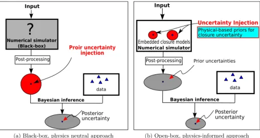
In addition to the parametric/non-parametric classification, it is possible to distinguish forward and backward methods, also referred to as data-free and data-driven approaches as illustrated inFig. 6. Forward (data-free) methods consist in propagating some pre-specified prob-ability distributions on the closure coefficients (or on the modeled terms) through the RANS equations and investigating the uncertainty distribution of the solution (Fig. 6a). On the other hand, backward (data-driven) methods consist in assimilating available data to infer the coefficient distributions or model errors (Fig. 6b). Such inferred dis-tributions then become available for propagation through the RANS equations in a subsequent prediction step as in the forward analysis. The applicability of the calibrated RANS models to new flows remains as a main concern for both parametric and non-parametric approaches.

Table 1shows a classification of the literature based on their para-metric/non-parametric and forward/backward characteristics. Note that the classification omitted data-driven methods that primarily fo-cused on developing turbulence models [e.g., 46, 47] rather than quantifying their uncertainties. A roadmap is provided inFig. 5to help the reader navigate through this review.

The rest of the paper is organized as follows. A brief review of available techniques for uncertainty propagation, data assimilation and statistical inference is presented in Section 2. In Section 3 we review parametric and multi-model approaches, the latter of which partly ac-counts for model-form uncertainties. Section 4 is dedicated to non-parametric approaches, which target model-form uncertainties. For completeness, an overview of uncertainties in scale-resolving ap-proaches, and more specifically LES, are briefly reviewed in Sections 5. Finally, conclusions, future research, and perspectives are presented in Section 6.

2. Fundamentals of probability and statistics for uncertainty quantification

Probability and statistics lie at the core of most of the work re-viewed in this work. Therefore, we provide a brief overview of the relevant methods in this section in the context of quantifying and re-ducing RANS model uncertainties. Based on these foundations, we

3_{Here we have used the terminology (“parametric” and “non-parametric”)} rather liberally, which is closely related to, but not strictly consistent with, the standard terminology in the statistics literature. In statistics, parametric models refer to those parameterized by a finite set of parameters, while non-parametric models refer to those with infinite degrees of freedom (e.g., spatial random fields).

briefly introduce the algorithms used for uncertainty propagation (forward analysis) and Bayesian inference (backward analysis). In particular, we discuss some commonly used methods for exact and approximate Bayesian inferences.

2.1. Representation, sampling, and propagation of model uncertainties

In the probabilistic approach, the uncertain quantities of concern in the RANS model, such as the model coefficients, can be represented as random variables. A random variable Z is a scalar function that may take a range of possible values z, referred to as realizations. A vector of random variables Z=[ , , ]Z1 Zn, indexed by integers, is a random

vector. An example is the combination of coefficients in a RANS model. A random field Z x( ) is a field of random variables indexed by the spatial coordinatex_{. It is also referred to as stochastic process when the}

index is time coordinate t. Random field is a generalization of random vectors to the continuous limit. The true Reynolds stress field x( )and

the discrepancies in the RANS-modeled Reynolds stress rans( )x _are

examples of random fields in RANS model uncertainty quantification. A continuous random variable can be characterized by its prob-abilistic distributions such as cumulative distribution function or probability density function p z( ). Common quantities of interest in uncertainty quantification are statistical moments of the random vari-ables such as expectation [ ]Z and variance ar[ ]z, which can be ob-tained via integration over all possible outcomes of Z, e.g.,

Z z p z dz

[ ]= ( ) , _(5a)

Z z Z p z dz

ar[ ]₌ ( [ ])2 ( ) .

(5b) The expectations and variances of random vectors and random fields can be obtained by applying Equation(5)to each component thereof, recalling that random vectors and random fields are collections of random variables indexed by integers and real numbers, respectively. Moreover, a random vector is further characterized by its covariance matrix Kij= ov( ,Z Zi j), which represents the correlation among the components ofZ. A generalization of the covariance matrix of random vectors to random fields leads to covariance kernelK ( ,x x), which indicates the pair-wise covariance between the random variablesZ ( )x

andZ ( )x corresponding to locations x and x . The most commonly used covariance kernel for the random fields representing model dis-crepancies is the squared exponential kernel:

x x x x K l ( , ) exp | | 2 , 2 2 2 = (6) with σ and l indicating variance and length scale, respectively. Such a kernel implies that the correlation between two random variables de-pends on their corresponding indexing locations. The farther apart the two locationsx and x are, the smaller the correlation betweenZ ( )x

andZ ( )x is.

In this work, we consider a RANS-based CFD model M: ( ; ) y, which is parameterized by and maps the latent variables (e.g., geometry, boundary conditions) to an observable output y. The multi-dimensional random variable can be a vector of model coefficients in parametric approaches or a spatial field in non-parametric approaches, e.g., Reynolds stress field x( )or eddy viscosity field xt( ). Two types of analyses can be performed:

•

•

Fig. 6. Illustration of uncertainty propagation (forward analysis) and statistical

inference (backward analysis) in the context of RANS simulations. Uncertainty propagation (forward analysis) involves propagating specified prior distribu-tions on the input (e.g., angle of attack/AoA, Reynolds number, model coefficients, or modeled terms such as Reynolds stresses) through a RANS si-mulation code and investigate the uncertainties in the solutions (quantities of interests/QoIs, e.g., lift and drag coefficients). Statistical inference (backward analysis) involves assimilating available measurement data to reduce un-certainties in the aforementioned input (e.g., AoA or Reynolds number). The inferred input distributions can be subsequently propagated to make predic-tions on the QoIs.

Table 1

Classification of literature of RANS model uncertainty quantification based on parametric/non-parametric approaches and data-free (forward)/data-driven (back-ward) approaches. Works in multi-model approaches are listed along with parametric approaches.

Parametric Non-parametric

data-free (forward) (Turgeon et al. [48], 2001), (Dunn et al. [49], 2011) ((Platteeuw et al. [50],

2008) (Margheri et al. [51], 2014) (Schaefer et al. [52], 2016) Iaccarino [(Emory et al. [56], 2017) (Edeling et al. [53,54], 2013) (Iaccarino et al. [57], 2017) (Xiao et al. [55], 2017) (Mishra and58], 2017)

Multi-model: (Poroseva et al. [59], 2006) (Edeling et al. [60,61], 2014, 2018)

data-driven (backward) (Cheung et al. [62], 2011) (Kato et al. [63,64], 2013, 2015) (Margheri et al. [51], 2014) (Ray et al. [23,65], 2018, 2016) (Edeling et al. [60,61,66], 2014–2018) (Papadimitriou and Papadimitriou [67], 2015)

(Dow and Wang [42], 2011) (Singh and Duraisamy [43], 2016) (Xiao et al. [44], 2016) (Wu et al. [68] 2016) (Wang et al. [69], 2016) (Parish and Duraisamy [70], 2016)

input probability distribution of can be inferred. The result is the

posterior distribution p( | )D of given dataD, representing an updated distribution from the prior distribution p( ) after observing the data.

2.2. Uncertainty propagation (forward analysis)

Techniques to propagate uncertainties can be classified into two categories [see ref.71, Chapter 1.4]: spectral methods [72] and Monte Carlo (MC) methods [73]. Spectral methods discretize the uncertainty space of the random variables by using orthogonal basis functions. This is done in a similar way in which orthogonal basis functions (e.g., Fourier functions or orthogonal polynomials) are used for the spatial discretization of deterministic PDEs. In uncertainty quantification, spectral methods have faster statistical convergence but they depend on the smoothness of the prior and the function that maps the inputs to outputs. Another barrier for spectral methods is the “curse of di-mensionality”: the number of function evaluations needed to accurately describe the statistics increases exponentially with the cardinality of the parameter space. Monte Carlo methods, on the other hand, approximate the solution by using random samples from the input uncertainty space and are not adversely affected by its dimensionality. However, the convergence rate is uniformly slow at a rate of N_O( 1/2)_{, where N is the} number of samples [73].

While the Monte Carlo based uncertainty quantification seems straightforward, the slow convergence rate poses a major challenge in applications where the computational cost of propagating each sample is high, as is the case for CFD simulations. Accelerating the statistical convergence of Monte Carlo methods has been a topic of intensive re-search, and numerous techniques for variance reduction have been proposed. Examples include stratified sampling, Latin hypercube sam-pling [74], importance sampling, and control variate [73]. A recent development is multilevel Monte Carlo (MLMC) methods [75–77], where simulations on coarser meshes are used as control variate of those on fine meshes to reduce the variances. A generalization of MLMC has led to multi-fidelity Monte Carlos methods [78–80], where a se-quence of models with ascending fidelities (e.g., empirical formulas, panel methods, RANS, LES) are combined for input uncertainty pro-pagation, with lower-fidelity models used as control variate of higher fidelity models as in the MLMC methods. However, so far these methods have been primarily used for propagating input uncertainties and not model uncertainties. One difficulty associated with multi-level and multi-fidelity methods is the possible non-trivial interactions between

model uncertainties and numerical discretization uncertainties. Another approach for overcoming the difficulty of expensive model simulations are surrogate models or response surface methods. In these methods, a surrogate of the original model, e.g., in the form of splines, polynomial chaos, or neural networks, are first constructed based on data obtained by evaluating the original model M at a number of design

points. The surrogate models provide an approximate functional

map-ping M: y that replaces the true mapping M for use in the sub-sequent sample propagation. Once constructed, the surrogate models can be evaluated at negligible computational costs. However, as with spectral methods, a main difficulty for the surrogate model approach is the curse of dimensionality, which makes it impractical for high di-mensional input space.

2.3. Statistical inference (backward analysis)

Most of the works on inference of model uncertainties (referred to as backward analysis above) are based on Bayes’ theorem:

p p p p ( | ) ( | ) ( ) ( ) , = D D D (7)

which states that the posterior probability p( | )D is proportional to the prior p( ) and the likelihood p( | )D . The prior p( ) summarizes all available knowledge about θ before observing the dataD. The like-lihood function p( | )D represents the probability of observing the data from a process described by the modelM ( )parameterized by θ. In the context of RANS uncertainty quantification, evaluating p( | )D for a given realization of the model parameters θ involves running the CFD code and is thus a costly operation. Finally, p( )D is the total probability of observing the data, which normalizes the posterior probability.

2.3.1. Bayesian inference based on Markov chain Monte Carlo sampling

Theoretically, evaluating the posterior can be straightforward using the following procedure similar to the plain Monte Carlo sampling: (i) draw samples from the prior, (ii) evaluate the likelihood for each sample, and (iii) aggregate the samples to estimate the posterior. However, this is much more challenging than in the forward analysis above. In the forward analysis the probability distribution is known, and thus one can draw more samples from the high probability regions, e.g., by using stratified sampling [73]. In contrast, Bayesian inference involves sampling from the posterior, the high probability regions of which is not known a priori. For example, samples drawn from regions with high prior probability may turn out to have very small likelihood after an expensive model evaluation, which may lead to very small posterior probability (see Equation(7)). Therefore, plain Monte Carlo methods are rarely used due to its difficulty in efficiently targeting the high posterior regions. Instead, Markov chain Monte Carlo (MCMC) methods are commonly used, which are a class of sequential sampling strategies in which the next sampled state only depends on the current state. Such a strategy allows the sampling to focus on high probability regions with occasional excursion to low probability regions (tails). Given a target distribution, the MCMC algorithm samples from that distribution by constructing a Markov chain whose stationary dis-tribution coincides with the target disdis-tribution. A typical MCMC algo-rithm with Metropolis–Hastings sampling is detailed inAppendix A.2

and illustrated graphically inFig. 7.

While the MCMC is the golden standard of Bayesian inference and posterior sampling, a major challenge of its application is that it re-quires a large number of samples to achieve statistical convergence. Typically the required number of samples range from (10 )_O 5 _{to (10 )O} 6_,

with the specific number depending on the shape of the posterior dis-tribution and the effectiveness of the sampling. In CFD applications, each evaluation involves a simulation that takes hours or even weeks to run depending on the complexity of the flow configuration. For ex-ample, RANS simulations of a jet in crossflow, which is a geometrically simple yet industrially relevant case, needed (10 )_O 7 _{grid points and} Fig. 7. Illustration of Markov chain Monte Carlo sampling of a banana-shaped

posterior (shaded contour) in a two-dimensional state space. The sampled distribution is illustrated with the trace of past samples (dots) and the marginal distributions (histograms plotted on the horizontal and vertical axes). Image obtained by using the MCMC demonstration code (https://chi-feng.github.io/ mcmc-demo/) by Chi Feng of MIT.

(10 )4

O CPU hours to run on a high performance computing cluster [23,65]. Clearly, it is impractical to perform a full RANS simulation for each evaluation of likelihood in the MCMC sampling. This is not only due to the large number of required samples but also because of the

sequential nature of traditional MCMC algorithms – the next proposed

sample depends on the evaluated posterior at the current state. As in the uncertainty propagation discussed above, surrogate models are commonly used for likelihood evaluation in MCMC-based model uncertainty quantification to alleviate the high computational cost of RANS simulations [23,65,66]. Efficient sampling of high di-mensional spaces with MCMC is a topic of active research, with many methods proposed in the past few years, e.g., by adaptively constructing local approximations during the sampling and by using the likelihood to inform the sampling [see, e.g.,81,82].

Another difficulty arises from the physical constraints among the state variables (e.g., parameters in closure models or Reynolds stresses at different spatial locations), which is particularly relevant for RANS model uncertainty quantification. For example, in the parametric ap-proach such constraints on the parameters dictates that points in some regions in the state space may yield nonphysical solutions or fail to converge at all. Consequently, such regions should be excluded when using MCMC to sample the posterior. Again, this can be done by building surrogate models from simulation data [23,65,83]. The frac-tion of excluded regions increases exponentially with the dimension of the sample space. Finally, it is noted that such a surrogate approach is also restricted to state spaces with low dimensions.

2.3.2. Approximate Bayesian inference based on MAP estimation

The MCMC method provides the most accurate sampling of the posterior but requires a large number of samples. When the exact probability is not critical and only the low order moments such as the mean and the variance are important, various approximate Bayesian inference methods can be used [e.g., 84, 85]. These methods use maximum a posteriori (MAP) probability estimate to obtain the mode (peak) of the posterior and not the full posterior distribution.

The MAP estimate can be computed in several ways, among which the most commonly used are variational methods and ensemble methods. Both methods are used in data assimilation with a wide range of applications ranging from numerical weather forecasting to subsur-face flow characterization. Both variational methods and ensemble methods have been adopted for parameter inferences. To this end, the system state is first augmented to include both the observable, physical state _i( )t (e.g., velocities, pressure, and/or turbulent kinetic energy) and parameters (e.g., model coefficients or Reynolds stress dis-crepancies, which are not observable and need to be inferred). Specifically, z is written as a vector formed by stacking the unknown parameters and the physical states i:

z=[ , , ; ] ,_{1 n (8)}

where indicates vector transpose, and =[ ,1 2, , r]is a vector of r parameters. When computing the MAP estimate, the following objective function is to be minimized:

z z z J= [ ] + y H[ ] P 2 R 2 1 1 (9)

where P andRare the covariance matrices of the state z and the ob-servation errors, respectively, with A ₁₌ A _P 1A

P and R1

simi-larly defined;His the observation matrix, which maps the state space to the observation space, typically reducing the dimension dramatically. Its interpretation will be further detailed in the context of the ensemble Kalman filtering algorithm (seeAppendix A.3).

Obtaining the MAP estimate is equivalent to minimizing the cost function J in Equation(9)under the constraint imposed by the models describing the physical system (i.e., RANS equations in case of turbu-lent flows), during which the set of parameters minimizing the dis-crepancies between the prediction and the observation data is sought.

In variational methods the minimization problem is often solved by using gradient descent methods, with the gradient obtained with ad-joint methods. In contrast, ensemble methods use samples to estimate the covariance of the state vector, which is further used to solve the optimization problem. Variational methods have been the standard in data assimilation and still dominate the field, while ensemble methods such as ensemble Kalman filtering have matured in the past decades and are making their way to operational weather forecasting. Hybrid approaches combining both approaches are an area of intense research and have been explored in CFD applications [84].

Recently, ensemble Kalman filtering (EnKF) [86,87] has been widely used in inverse modeling to estimate model uncertainties [44,85]. In EnKF-based inverse modeling, one starts with an ensemble of model parameter values drawn from their prior distribution. The filtering algorithm uses a Bayesian approach to assimilate observation data (e.g., data from experiments and high-fidelity simulations) and produces a new ensemble that represents the posterior distribution. In parametric or field inference of concern here, the EnKF method is used in an iterative manner to find the states that optimally fits the model and data with uncertainties of both accounted for, which is essentially a derivative-free optimization. As such, it is referred to as the iterative

ensemble Kalman method. This is in contrast to the EnKF-based data

assimilation as used in numerical weather forecasting, where the ob-servation data arrive sequentially. The algorithm for the iterative en-semble Kalman method is presented inAppendix A.3.

EnKF has some well known limitations due to its assumptions of linear models and Gaussian distributions, and theoretically they would perform poorly for non-Gaussian priors and highly nonlinear forward models. However, despite the above-mentioned limitations, EnKF methods have been successfully used in a wide range of applications. Mathematicians have performed analyses to shed light on why they have worked well in view of their theoretical limitations [88,89].

3. Parametric and multi-model approaches

In this review we use “parametric approaches” to refer to methods that quantify the uncertainty associated with RANS simulations by in-vestigating primarily the sensitivity of the results to the closure coef-ficients. As mentioned in Section1, we will use “forward approaches” to refer the methods that consist of perturbing the closure coefficient ac-cording to some probability distribution function and quantifying the output uncertainty on the computed solution. This is in contrast to “backward approaches”, in which observations are used to infer the model coefficients. In both the forward and backward approaches, the model structure is fixed and only the uncertainty on the coefficients is quantified. This can nevertheless be used to learn about structural in-adequacy of the model, as will be shown later. In some cases, one of the outcomes of the inference process is an estimate of the plausibility of a given model based on the available observations, i.e. the inference may also provide some guidelines for model selection. Finally, we will dis-cuss multi-model approaches in which the uncertainty on the model choice is tackled by considering a set of alternative model structures.

3.1. Uncertainties in RANS model parameters

All RANS models have some closure coefficients. A typical example is provided by the well-known k–ε model, initially proposed by Jones and Launder [90]. In this model, the Reynolds stress tensor is modeled by using the Boussinesq approximation in Equation(4), and the tur-bulent viscosity t is computed by solving additional transport

equa-tions for the turbulent kinetic energy k and the turbulent dissipation ε:

C k

t µ

2

k t U k x x k x i i k i t k i + =P + + (10b) t Ui xi C k k C k xi x , t i 2 1 2 + = P + + (10c) wherePkis the production of turbulent kinetic energy through energy

extraction from the mean flow gradient:

S : ,S

k= ij ij

P ₍₁₁₎

and the double dot ":" indicates tensor contraction.

The k–ε model above involves coefficientsCµ,C1,C2, k, and . The

nature of these coefficients leads to ambiguity regarding their values, and a set of flow-independent optimal values are unlikely to exist [66]. The above-mentioned coefficients are traditionally calibrated to re-produce results of a few canonical flows. One of such canonical flows is the decaying homogeneous isotropic turbulence. In this flow the k and ε equations(10b) and (10c)simplify to

dk dt = , (12) d dt C k and 2 . 2 = ₍₁₃₎

These equations can be solved analytically to give

k t k t t ( ) , n 0 0 = (14) with reference time t0=nk /0 0and the exponent n=1/(C2 1), the

latter of which leads to:

C n

n

1 .

2= + ₍₁₅₎

The standard value for n is such thatC2=1.92. However, this is by no

means a hard requirement and other models do use different values for C2. For instance, the RNG k–ε model uses a modified value C˜2=1.68,

and the k–τ model (essentially a k–ε model rewritten in terms of

k/

= ) uses C2=1.83[91]. Nevertheless, experimental results suggest that most data agrees withn=1.3, which corresponds toC2=1.77

[92].

The coefficient Cµ is calibrated by considering the approximate

balance between production and dissipation which occurs in free shear flows or in the inertial part of turbulent boundary layers. This balance can be expressed as U x C k U x . k t 1 µ 2 2 ₂ 1 2 2 = = = P (16) Here, indices 1 and 2 indicate coordinates in streamwise and wall-normal directions, respectively. Equation(16)can be manipulated to-gether with the turbulent-viscosity hypothesis 12= t U1/ x2 to yield

U x

( / )

12= 1 2 1, which in turn yields C k . µ 12 2 = (17) DNS data [93] were used to show that 12 0.30k(except close to the

wall), and thus Cµ=0.09 is the recommended value [94]. Again, however, different models use different values forCµ. For example, it

was found that Cµ 0.085in the case of the RNG k–ε model.

Another fundamental flow to be considered is the fully developed plane channel flow, which implies that Dk Dt D Dt/ = / =0. The re-sulting simplified governing equations leads to the following constraint among several parameters [94]:

Cµ (C C ),

2 1/2

2 1

= ₍₁₈₎

where κ is the von Karman constant. It should be noted that the nominal coefficients in the k–ε model satisfy this constraint only approximately, leading to 0.43, instead of the standard value of =0.41. However, even the “standard values” has been questioned recently, with κ de-termined to fall in the range [0.33, 0.45] based on experimental data in the literature [95].

The following constraint betweenC1andC2can be found by

ma-nipulating the governing equations of uniform (i.e., U x1/ 2=constant) shear flows [94]: C C 1 1. k 2 1 = P (19) Tavoularis and Karnik [96] measuredPk/ for several uniform shear flows and reported values between 1.33 and 1.75, with a mean around 1.47. Note, however, that Equation(19)becomes 2.09 with the stan-dard values forC1andC2, which is significantly different from the

mentioned experimental values. Note that, regardless of the un-certainties, the coefficients have to satisfy the constraint C2>C1as has

been shown through numerical experiments by Ray et al. [23]. The physical reason behind this delineation is that the ratio C C2/ 1

corre-sponds to the spreading rate of a free jet. A ratio of C C2/ 1<1, or equivalently C2<C1, would lead to contracting jet, which is

non-physical [97].

The parameter kcan be considered a turbulent Prandtl number and

represents the ratio of the momentum eddy diffusivity and the TKE diffusivity. These quantities are usually close to unity, which is why the standard value for k is assumed to be 1.0. However, no experimental

data can be found to justify this assumption [50], leading to a range of recommended values among the different variations of the k–ε model. For instance, the RNG k–ε model uses k=0.72[10]. The parameter controls the diffusion rate of ε, and its value can be determined by using the constraint imposed by Equation(18), i.e.

C_µ (C C ). 2 1/2 2 1 = (20)

Fig. 8. Flow past a backward facing step at Reh=50000. Sensitivity of the k–ε model to the closure coefficients. Plots of the skin friction and its sensitivities versus the longitudinal position behind the step. Figures reproduced with permission from Turgeon et al. [48].

Similar uncertainties affect the coefficients of other turbulence models. Margheri et al. [51] discuss in further detail the uncertainties in the coefficients of the k–ε model and Menter's SST k–ω model [98] and characterized their probability distributions by using generalized polynomial chaos approximations of extensive literature databases. Recently Shaefer et al. [99] also investigated the uncertainties in the coefficients of the SA model [100], Wilcox’ k–ω model, and the SST k–ω model, pointing out the large epistemic intervals on their values.

3.2. Parametric uncertainty in RANS models: forward approaches

In light of the scattering in closure coefficients of RANS models as reviewed above, several uncertainty quantification (UQ) analyses have focused on quantifying the effect of such uncertainties on the output quantities of interest (QoI). Among the pionneering efforts on forward sensitivity analysis of RANS models is the work of Turgeon et al. [48]. They investigated the effect of uncertainty in theCµ,C1,C2, kand of

the standard k–ε turbulence model (combined with wall functions) on the solution output. The uncertainty analysis was based on a general-ized sensitivity equation method [101], i.e. using sensitivity derivatives to propagate uncertainties in the turbulence model coefficients to the solution. In these papers, the uncertainty intervals of the turbulence coefficients are taken arbitrarily, since finding information about the range of uncertainty in the coefficients is not straightforward. The re-sults presented for the flow past a flat plate and the flow over a back-ward-facing step, which is a severe configuration for RANS models, show that the uncertainty in the model coefficients is not sufficient to account for the observed discrepancies between the predictions and the measurements. An interesting by-product was the identification of the most influential parameters based on the scaled sensitivities. For the flow over a backward-facing step, parametersC1andC2are found to

exert the strongest influence on the wall friction coefficient Cf and thus

on the reattachment point location.Fig. 8shows the nominal prediction and the uncertainty range for the distribution of Cf downstream of the

step (panel a) and of its scaled sensitivities (panel b), defined as

Cf Cf ,

j nom,j

=

where jis the j-th model parameter and nom,jis its nominal value. The

method was finally applied to an airfoil flow, showing the increasing sensitivity of the solution to the RANS coefficient for larger angles of attack.

Sensitivity-based analyses provide only an uncertainty band around the nominal solution. To obtain more information about the uncertainty of the solution, and specifically its full probability distribution given some input joint probability of the model parameters, UQ techniques (e.g., the MC method presented inAppendix A.1) can be used to pro-pagate an assigned joint distribution on the closure coefficients across the model. For instance, Platteeuw et al. [50] used experimental da-tabases and DNS results, along with physical constraints on the

coefficients to construct realistic a priori approximations of the input distributions for the different coefficients of the standard k–ε with wall functions [102]. Their final set of uncertain coefficients includes the model parametersCµ,C2, k, the wall function parameters κ (i.e. the

von Karman constant), and the log-law constant, as well as the turbu-lence intensity imposed at the free-stream boundary. A probabilistic collocation method was used to efficiently propagate the input joint distribution through a zero-gradient flat plate flow configuration. Mean flow variations as a consequence of the turbulence model uncertainty were found to be large enough (at least compared to numerical errors) to encompass the experimental data available for the friction coefficient distribution along a flat plate. They also carried out a sensitivity ana-lysis of the output QoI, showing that the solution was more sensitive to the wall function parameters than to other model parameters.Fig. 9

shows the uncertainty range obtained by assigning a normal probability density to the von Karman constant, N(0.417, 0.0127), while keeping other parameters constant. The most probable solution is in slightly better agreement with the experimental data. On the other hand, the predicted uncertainty interval encompasses the data.

Forward UQ for the k–ε turbulence model with wall functions was also carried out by using the Latin hypercube sampling method [49]. This was used to propagate distributions of the input coefficients esti-mated from the data from Pope [94] for the flow past a backward-facing step, and the mean values were reported for the flow output parameters of interest along with their associated uncertainties. The results showed that model coefficient variability had significant effects on the streamwise velocity component in the recirculation region near the reattachment point and turbulence intensity along the free shear layer. The reattachment point location, pressure, and wall shear were also significantly affected.

In the above-mentioned works, the uncertainty distributions of the input parameters were all obtained in a largely subjective manner. The specification of such prior distribution has an impact on the output probability distributions. To reduce such uncertainties it is possible to use analytical relationships allowing to express the closure coefficients in terms of basic properties of canonical flows (e.g., the power-law exponent of the free decay of turbulent kinetic energy in isotropic turbulence). Following this idea, Margheri et al. [51] carried out an extensive literature survey and collected a large amount of experi-mental and numerical data characterizing the input coefficient dis-tributions for the Launder–Sharma low-Reynolds number k–ε and Wilcox k–ω models. The collected data exhibited a significant scat-tering, which confirmed the hypothesis that the uncertainties in the measured or computed basic flow properties leads to uncertainties in the RANS model coefficients.Fig. 10reports the resulting input prob-ability density function (pdf) for the parameters of the k–ε model, which are reconstructed by using the generalized polynomial chaos (gPC) expansion [103]. The input distributions were propagated through the RANS equations applied to a turbulent channel flow for two different friction Reynolds numbers, Re =950and Re =2000, showing that both models give inaccurate predictions of the intensity and peak

Fig. 9. Distribution of Cffor the flow along a semi-infinite flat plate with zero pressure gradient and 99% uncertainty interval. Sensitivity of the k–ε model to the von

location of the turbulent kinetic energy. The observed inaccuracies were ascribed to structural uncertainties of turbulence models, which are not accounted for by the parametric data-free approaches.

3.3. Parametric uncertainty in RANS models: backward approaches 3.3.1. Statistical inference of model parameters

Forward parametric approaches strongly rely on the availability of reliable data for constructing the coefficient probability intervals or joint distributions. Unfortunately this information is inevitably in-complete and subject to errors. Additionally, it remains restricted to rather simple flow configurations, and it is difficult to extend such data for robust predictions of different flows. Finally, data are only available for observable quantities (e.g., pressures and velocities) and not for the closure coefficients themselves. However, an inverse statistical problem can be solved to infer the input coefficients and possibly their un-certainties. Once obtained, this information can be propagated back through the model to estimate uncertainty intervals on the output QoIs. The inverse statistical problem can be solved by using a determi-nistic or probabilistic approach. In the determidetermi-nistic approach, a set of optimal closure coefficients is obtained by minimizing the model error with respect to some reference data. For instance, Margheri et al. [51] utilized the gPC response surfaces generated for their forward UQ analyses to find optimal combinations of model coefficients that lead to minimum global error on the mean and friction velocities with respect to DNS data for the turbulent channel flow case. Their findings suggest that the values of the model coefficients recommended in literature, which are generally set as default in commercial and open-source CFD

codes, do not fall within the best-fit range. Note however that such deterministic estimates do not provide information on the variability of the optimal coefficients or their validity for a different flow case.

In order to quantify and reduce the uncertainties on model coeffi-cients while simultaneously providing an estimate of model-form un-certainties, it is possible to use Bayesian inference techniques as in Section2.3. In such an approach, a priori knowledge or assumptions about the coefficients is updated by using available data. When data are highly uncertain or sparse, the updated information will exhibit little difference from the prior distribution. As more data arrive, it is possible to further update the model, thus refining the initial estimate. In the Bayesian calibration process, a key ingredient is the likelihood function in Equation(7), which may carry information about observational noise on the data and model-form uncertainty. The latter being the gap be-tween the average model predictions and the “truth”, as will be dis-cussed later in Section 3.3.2.

Cheung et al. [62] performed the first application of Bayesian un-certainty quantification techniques for calibrating turbulence models and making probabilistic predictions for new flows. They used MCMC sampling to carry out Bayesian calibration of the Spalart-Allmaras model from velocity and skin friction data for three boundary layers with zero, adverse, and favorable pressure gradients. This effort en-abled the estimation of the whole posterior joint probability distribu-tion of the coefficients (instead of deterministic values) as well as a comparison of competing models for the likelihood function (noted M1,

M2, andM3) relating the observed data to the model output. As an

ex-ample,Fig. 11shows the marginal posterior distributions obtained for the von Karman constant κ and the coefficient c,1, along with their joint Fig. 10. Normalized probability density function (pdf/max(pdf)) of the Launder–Sharma k–ε model coefficients recovered through gPC. Figures reproduced with

scatter plot when using the stochastic model M3. Bayesian calibration is

able to discover a posterior correlation between these two parameters, showing the importance of calibrating all parameters simultaneously. The MCMC-based calibration process involved a large number of boundary layer calculations (32,768 samples), each based on a full Navier–Stokes incompressible flow solver. Ray and co-workers [23,65,104,105] used a similar approach to infer the model coefficients for a more complex configuration, namely, a jet-in-cross-flow. For ex-ample, experimental data were used to calibrate the parameters in a nonlinear eddy viscosity model [23], where surrogate models were used to reduce the computational burden of the MCMC sampling.

Kato and Obayashi [63] used ensemble Kalman filtering [86,106] to determine the values of the parameters of the Spalart–Allmaras turbu-lence model for the zero-pressure gradient flat plate boundary layer at

M=0.2 and Re 5 10_{= ×} 6_{. The data were velocity profiles and wall}

pressures generated by the same model using a known set of coefficients (equal to the nominal ones). An advantage of using synthetic data is to remove structural uncertainty, since the trained model is the same used to generate the data. The results show the ability of the EnKF method to identify the correct model parameters for a relatively low computa-tional cost (ensembles of 100 function evaluations, i.e. CFD calcula-tions). The approach has been extended to more complex flows around airfoils [64], establishing a general framework for combining experi-mental fluid dynamics and CFD for predictions.

An even more efficient way of finding the optimal coefficients is to maximize the likelihood function by using gradient-based methods. This corresponds to finding the set of closure coefficients corresponding to the maximum probability of observing the data. The main drawback of this approach is that only deterministic sets of coefficients are

obtained as an outcome of the calibration. Papadimitriou and Papadimitriou [67] obtained variance estimates of the optimal coeffi-cients by using the Hessian of the likelihood function with respect to the parameters θ. They found that the posterior variance due to the overall observational uncertainty (e.g. to the discrepancy between the model output and the data) plays a dominant role. This indicates that coeffi-cient calibration alone is not sufficoeffi-cient to match the data, and that the bias introduced by the model structure is mostly responsible for the discrepancy. Unfortunately, Hessian calculations require computing the second sensitivity derivatives of the model with respect to the para-meters, which is a highly intrusive and delicate task and is not com-patible with black-box Navier–Stokes solvers.

Bayesian strategies similar to that of Cheung et al. [62] can also provide estimates of the uncertainty associated with the model form, grounded in uncertainties in the space of model closure coefficients. This can be achieved by calibrating the model separately against several sets of data. The spread in the posterior estimates of closure coefficients across calibration scenarios provides a measure of the need for read-justing the model coefficients to compensate for the inadequacy. An example of such a sensitivity study is given by Edeling et al. [66], where the Launder–Sharma model was calibrated separately against 13 sets of flat-plate boundary layer profiles from Kline et al. [107]. The results showed a significant variation in the most-likely closure-coefficients values for the different pressure gradients, despite the relatively re-stricted class of flows (flat plate boundary layers) considered for the calibrations.

The main lessons learned from the preceding exercise are: (i) there are no universal values for the closure parameters of the turbulence models; (ii) the parameters need to adjust continuously when changing

Fig. 11. Calibration of the Spalart–Allmaras model from the flat plate flow data, showing (a) the posterior distributions and (b) scatter plots of the inferred