Science Arts & Métiers (SAM)
is an open access repository that collects the work of Arts et Métiers Institute of Technology researchers and makes it freely available over the web where possible.
This is an author-deposited version published in: https://sam.ensam.eu Handle ID: .http://hdl.handle.net/10985/13719
To cite this version :
Rémi CURTI, Philippe LORONG, Guillaume POT, Stéphane GIRARDON - How to model orthotropic materials by the Discrete Element Method (DEM): random sphere packing or regular cubic arrangement? - Computational Particle Mechanics - Vol. 6, n°2, p.145-155 - 2019
How to model orthotropic materials by the
Discrete Element Method (DEM): random
sphere packing or regular cubic
arrangement?
Rémi CURTIa, Stéphane GIRARDONa, Guillaume POTa, Philippe LORONGb
aArts et Métiers, LaBoMaP, EA 3633, rue Porte de Paris, 71250 Cluny, France bArts et Métiers, PIMM, UMR CNRS 8006,151 boulevard de l’Hôpital, 75013
Paris, France
(+33)6 76 31 31 90
ORCID number : 0000-0002-8997-9248
Abstract
The discrete element method (DEM) is used for continuous material modeling. The method is based on discretizing mass material into small elements, usually spheres, which are linked to their neighbours through bonds. If DEM has shown today its ability to model isotropic materials, it is not yet the case of anisotropic media. This study highlights the obstacles encountered when modeling orthotropic materials.
In the present application, the elements used are spheres and bonds are Euler-Bernoulli beams developed by André et Al. [1]. Two different modeling approaches are considered: cubic regular arrangements, where discrete elements are placed on a regular Cartesian lattice, and random sphere packed arrangements, where elements are randomly packed. As the second approach is by
definition favoring the domain’s isotropy, a new method to affect orientation-dependent Young’s modulus of bonds is proposed to create orthotropy. Domains created by both approaches are loaded in compression in-axis (along the material orthotropic directions) and off-axis to determine their effective Young’s modulus according to the loading direction.
Results are compared to the Hankinson model which is especially used to represent high orthotropic behavior such as encountered in wood or synthetic fiber materials. For this class of materials, it is shown that, contrary to cubic regular arrangements, the random sphere packed arrangements exhibit difficulties to reach highly orthotropic behavior (in-axis tests). Conversely, this last arrangements display results closer to continuous orthotropic material during off-axis tests.
Keywords
1. Introduction
Modeling of continuous media using a particle approach such as DEM (Discrete Element Method) is recent. It started in the early 2000’s with aggregates modeling [2–4]. The transition from continuum towards particle models requires
considering the interactions between particles not as simple contacts but as “cohesive bonds” having a more complex behavior. Two main aspects of these bonds have to be taken into account: their “force model” and their fracture conditions (if the modeled media is brittle). The force model is used to compute interaction forces between two elements/particles based on their relative positions. It can also include damping, plasticity or other physical behavior. The fracture condition can be either based on bond deformation, interaction forces or both. For each particle, resulting forces are calculated according to the boundary conditions of the simulated system and to other interacting elements, called its “neighbors”. Then Newton’s Law of Dynamic is solved with an explicit scheme leading to element’s acceleration. New position of the element for the next increment is approximated by integrating its acceleration. In the present study, the integration is done thank to a velocity Verlet algorithm [5]. This approach derived from molecular dynamics [6], was initially developed to model granular media [7]. It exhibits several advantages toward FEM in order to simulate cutting or fracture of materials. It allows indeed modeling these phenomena with high robustness and as meshless methods as a discrete method, does not require mesh update nor pre-crack location.
The DEM has already been applied for modeling continuous materials presenting an isotropic and homogeneous behavior [8,9]. It can deal efficiently with
heterogeneity of the media and inclusions when required, both in elasticity and fracture mechanics [10,11]. It even allows to investigate the behavior of original structure composed both of granular and continuous media [12]. Nonetheless, it is also of high interest to deal with anisotropic materials such as fiber-reinforced materials, or natural composites such as wood. DEM is suited for the modeling of dynamic and complex loadings of these materials, for instance crash [13] or machining. Artificial or natural composites are highly orthotropic materials. Their elastic modulus in fiber direction is much higher than their moduli in transversal
directions, with a ratio between these moduli that can reach one hundred. However, the numerical modeling of these materials with particle approaches, such as the DEM, is more difficult compared to isotropic media. This comes from the difficulty to define bond behavior in order to reproduce the sought-after anisotropy. The modeling of orthotropic elastic behavior with the DEM constitutes the main objective of this paper.
In the DEM, as previously said, the constitutive laws must be implemented in the bonds between discrete elements (DE) rather than in a stiffness matrix like in FEM. In the case of orthotropic behavior, several methods are already
experimented in the literature for various purposes. One of the most encountered is the use of regular arrangement, where elements are intentionally lined up along the privileged directions of the material forming a regular Cartesian grid [14–16] or user designed regular pattern [17]. By this way, the orthotropic behavior of the material is rebuilt thank to the structure of the domain. A different strategy suggested by [18] consists in using compact domains, where elements are randomly placed and packed by a compacting script [19]. Then, bonds are generated between elements in contact except the bonds within a certain angle range around a given direction. Thereby, in this direction, the lack of bonds reduces the Young’s modulus and generates anisotropy in the domain. An intermediate way of proceeding is to model fibers and matrix by using either regular or randomly packed elements [20,21]. This last approach requires elements quite smaller than the fiber radius. As the amount of elements
composing a model impacts drastically the computation time, only small domains can be studied with such an approach. In the literature, to the best knowledge of the authors, the approaches set up to obtain anisotropy are not confronted. In this paper, the elements are spheres, and the bonds behave as Euler-Bernoulli beams [1]. Two different arrangements are compared in order to reach an orthotropic elastic behavior: regular cubic arrangement for its popularity in the literature, and a new method, based on packed arrangement, where beams
Young’s Moduli depend on bonds orientation. In comparison with the methods of the literature this method avoids to simply delete bonds and lower their quantity. The ability of these two arrangements to match the expected material elastic orthotropic properties is compared along their three main directions of orthotropy,
and also under off axis loading. The Hankinson’s equation [22] is used to define the direction dependent reference value of Young’s modulus. Simulations were run under quasi-static loading with GranOO workbench (1.0) [1] with the only addition of a developed plugin to affect the bonds elastic properties. The
orthotropic dynamic behavior as well as fracture and anelastic behaviors are not discussed in this study.
2. Material and method
2.1. DEM Models
As described in the introduction, DEM requires the use of bonds to bear the material behavior. The bonds model chosen is Euler Bernoulli cylindrical beam [1]. The beams elastic behavior depends on four parameters: Young modulus (𝐸𝑏), radius ratio (𝑟̃𝑏), length ( 𝑙𝑏), and Poisson ratio (𝜈𝑏). The radius ratio equals to the beam cross-section area divided by the mean radius of the two interacting elements (spheres). Euler-Bernoulli beams have three modes of deflection: compression/tension, flexion and torsion. The Poisson ratio allows computing the shear modulus in torsion. The radius ratio brings scalability of the model
regarding the discrete element dimensions. If the size of elements is modified, the section and the length of beams will change accordingly resulting in an equivalent behavior of the built domain. In the study conducted in this article, the radius ratio is maintained equals to unity to focus only on the beam Young’s moduli impact on the global domain properties. In depth properties of those bonds are explained by [1]. In addition, numerical damping (𝜂) is added in the beams behavior in order to avoid endless oscillations around equilibrium state during simulations. The use of Euler-Bernoulli beams allows a fine tuning of the material behavior with a small number of parameter compared to commonly used spring/damper models, at the expense of the understanding of each parameter impacts due to their inter-dependency. Both the stiffness in compression and the stiffness in bending of the bond depend on the same parameters: its Young’s modulus and its cross-section. Regular arrangement
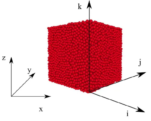
In cubic regular arrangements, also called simply “regular” arrangements in the following, spherical elements are regularly spaced along edges of a cubic frame
(see Fig. 1). The directions of edges correspond to the material principal directions (𝑖,⃗ 𝑗 , 𝑘⃗ ). Elements have all the same shape and properties. Their two parameters are their radius and their density (ρ). The density depends on the volume fraction of the model (ratio between the volume occupied by the elements and the whole represented volume). This parameter only impacts the dynamic behavior of the domain and not the static response, so its impact is not
investigated in this article. The beams binding elements together are only lined up with the three main directions of the arrangement. They present three different sets of parameters depending on their direction: (𝐸𝑏𝑖, 𝑟̃𝑏𝑖, 𝜈𝑏𝑖, 𝑙𝑏) along 𝑖,⃗ (𝐸𝑏𝑗, 𝑟̃𝑏𝑗,
𝜈𝑏𝑗, 𝑙𝑏) along 𝑗,⃗⃗ (𝐸𝑏𝑘, 𝑟̃𝑏𝑘, 𝜈𝑏𝑘, 𝑙𝑏) along 𝑘 ⃗⃗⃗ . Only the initial length 𝑙𝑏 remains mandatorily identical from one beam to another, whatever its direction is, since the initial length is the distance between two regularly spaced interacting elements centers.
In regular arrangements, beams properties can be analytically calibrated to obtain desired structure in-axis properties, for instance Young’s modulus Ei, Ej and Ek, in
the material principal directions:
𝐸𝑖 ∙ 𝑆𝑖 = 𝐸𝑏𝑖 ∙ ∑𝑆𝑏𝑖, 𝐸𝑗∙ 𝑆𝑗 = 𝐸𝑏𝑗∙ ∑𝑆𝑏𝑗, 𝐸𝑘∙ 𝑆𝑘 = 𝐸𝑏𝑘 ∙ ∑𝑆𝑏𝑘 (1) where 𝑆𝑖, 𝑆𝑗, and 𝑆𝑘 are the cross-section of the domain with respectively 𝑖,⃗ 𝑗 , 𝑘⃗ as a normal, and ∑𝑆𝑏𝑖, ∑𝑆𝑏𝑗, ∑𝑆𝑏𝑘, the area occupied by beams section in this
domain cross-section.
As previously said the radius is equal to 1 and thus, as all elements have the same radius, all the bonds have the same radius and section 𝑆𝑒 = 𝑆𝑏𝑖 = 𝑆𝑏𝑗 = 𝑆𝑏𝑘. Then equation (1) becomes, by isolating Eb and writing respectively 𝑛𝑖, 𝑛𝑗, 𝑛𝑘 the
amount of elements in the planes (𝑗,⃗⃗ 𝑘⃗ ), (𝑖,⃗ 𝑘⃗ ), and (𝑖,⃗ 𝑗 ), 𝐸𝑏𝑖 = 𝐸𝑖∙ 𝑆𝑖 𝑛𝑗 × 𝑛𝑘 × 𝑆𝑒, 𝐸𝑏𝑗 = 𝐸𝑗∙ 𝑆𝑗 𝑛𝑖 × 𝑛𝑘 × 𝑆𝑒, 𝐸𝑏𝑘 = 𝐸𝑘∙ 𝑆𝑘 𝑛𝑖 × 𝑛𝑗 × 𝑆𝑒. (2) Packed arrangement
An example of random sphere packing arrangement, which will be named packed arrangement for readability, is given on Fig. 2. An important difference between regular and random sphere packing arrangement is the absence of bonds
principal directions (𝑖,⃗ 𝑗 , 𝑘⃗ ). It is thus not as simple as for the regular arrangement to define the Young modulus of each beam. The proposed method is to deduce beams’ Young’s modulus from an interpolation between Ebi, Ebj and Ebk. This
interpolation depends on beam’s spatial orientation, which is defined by the spherical coordinates 𝜃 and φ, respectively the polar angle and the complimentary angle of the azimuthal angle (see Fig. 3). In DEM, the orientation of the bond linking two elements is defined by its branch vector: vector starting on one element center O1 and pointing out the second element center O2. Note that 𝑝 is the projection of the branch vector 𝑂⃗⃗⃗⃗⃗⃗⃗⃗⃗⃗⃗ onto the plane (O1𝑂2 1, 𝑗,⃗⃗ 𝑘⃗ ).
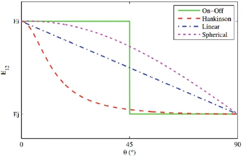
Four laws to set Young’s modulus 𝐸12 of the bonds of packed domains between two given discrete elements “1” and “2” are investigated in this article:
On-Off:
𝐸12 = 𝐸𝑏𝑖 𝑜𝑟 𝐸𝑏𝑗 𝑜𝑟 𝐸𝑏𝑘 (3) if 𝑖,⃗ 𝑗 or 𝑘⃗ is the closest direction.
Hankinson’s equation: 𝐸12 = 𝐸𝑏𝑖∙𝐸𝑝⃗⃗ 𝐸𝑏𝑖∙sin2𝜃+𝐸𝑝⃗⃗ ∙cos2𝜃 (4) with 𝐸𝑝 = 𝐸𝑏𝑗∙𝐸𝑏𝑘 𝐸𝑏𝑗∙sin2𝜑+𝐸𝑏𝑘∙cos2𝜑 (5) the modulus in 𝑝 direction.
Linear: 𝐸12 = 𝐸𝑏𝑖+ (𝐸𝑏𝑗− 𝐸𝑏𝑖) ∙𝜃𝜋 2 + (𝐸𝑏𝑘− 𝐸𝑏𝑗) ∙ 𝜃∙𝜑 (𝜋2)2. (6) Spherical:
𝐸12 = cos(𝜑) ∙ 𝐸𝑏𝑖+ 𝑐𝑜𝑠(𝜃) ∙ sin(𝜑) ∙ 𝐸𝑏𝑗+ sin(𝜃) ∙ 𝑠𝑖𝑛(𝜑) ∙ 𝐸𝑏𝑘. (7)
Fig. 4 shows the aspect of these four laws for 𝜃 = 0.
Hankinson’s equation [22] is a very common approximation of off-axes properties in composites or wood and already used in FEM or analytical model to predict Young’s moduli according to fiber angle [23]. Spherical, On-Off and linear interpolations are not physics-based laws but their very simple implementation
justifies their trial. Except linear interpolation, all chosen laws offer the advantage to commute: Eb depends on the values of Ebi, Ebj and Ebk but not on the order they
are taken for its calculation. 2.2. Simulation process
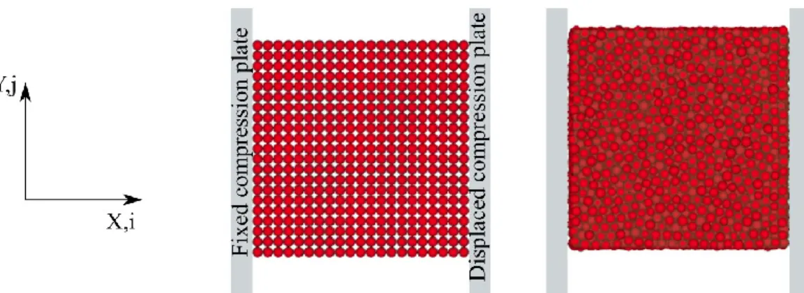
To obtain the mechanical properties of the structure, an unidirectional
compression test has been modeled (see Fig. 5 and Fig. 6). The loading direction is denoted 𝑋 ⃗⃗⃗ and can be different from material’s principal directions. Four parameters are recorded during the simulation: reaction force F on the plates according to the loading direction, strain 𝜀𝑥, of the domain in the 𝑋 ⃗⃗⃗ direction,
kinetic energy and potential elastic energy of the system. Forces and strains are then post-treated in order to calculate the global Young modulus Ex in the
𝑋
⃗⃗⃗ direction from equation (8). 𝐸𝑥= 𝑆𝐹
𝑥∙𝜀𝑥 (8)
𝑆𝑥 is the area of the domain section which is measured prior to the simulation. 𝜀𝑥
computation is explained in section 2.5.
Data is recorded every increment. The optimal time step of one increment is automatically computed by an inbuilt Granoo algorithm according to the beams stiffness. As computations are done in dynamics, it is also verified that when modulus is calculated, kinetic energy of the domain is negligible toward its elastic deformation energy (more than four decades of difference).
2.3. In-axis loading
For in-axis loading the simulations are conducted on discretized 10-mm cubes whose frame (𝑋 ⃗⃗⃗ , 𝑌⃗ , 𝑍 ) and material principal directions frame (𝑖,⃗ 𝑗 , 𝑘⃗ )
correspond. They are successively loaded along 𝑋 , 𝑌⃗ then 𝑍 by a mobile plate compressing the domain against a fixed one, without friction, until they reach 5% deformation in the loading direction. The setup is presented in Fig. 5.
2.4. Off-axis loading
Eight supplementary regular domains are designed to present a α-rotated frame (𝑖,⃗ 𝑗 , 𝑘⃗ ) from 10° to 80° by 10°-steps around 𝑍 to highlight mechanical behavior
when load is off-axis. The loading direction is 𝑋 ⃗⃗⃗ . For example, Fig. 6 displays a 20°-rotated regular cubic domain under off-axis loading. On the contrary to regular arrangements, the packed arrangement remains the same. However, bond properties are recalculated toward the new material frame orientation for every interpolation law given in 2.1. The packed model is also loaded in the height new cases.
2.5. Strain measurement
In order to compute 𝜀𝑥 it is necessary, in the DEM model, to calculate an average of the relative displacements between elements. For this average, elements interacting with the compression plates are not taken into account. This choice is justified by the specimen’s geometry. Indeed, rotated domains faces are “stair” shaped (see Fig. 6 above), thus, only some elements are in contact with the two plates and strains are not homogeneous when too close to the plates.
Under the hypothesis of a homogeneous strain field in the remaining portion of the domains, the displacement 𝑈𝑥𝑒 of one discrete element 𝑒 in the direction 𝑋
with respect to the fixed compression plate depends linearly on the deformation 𝜀𝑥 and can be written as:
𝑈𝑥𝑒 = 𝑋
0𝑒∙ 𝜀𝑥+ 𝐶𝑠𝑡, (9)
where 𝑋0𝑒 is the initial position of one element along 𝑋 ⃗⃗⃗ and 𝐶𝑠𝑡 is a constant
whose value depends only of the position of the frame origin.
The strain 𝜀𝑥, which is minimizing the ordinary squared difference [24] between
the approximation 𝑈𝑥𝑒 and the measured displacement 𝑈
𝑥 of one element is
calculated as stated in (10):
𝜀𝑥= 𝑐𝑜𝑣𝑎𝑟𝑖𝑎𝑛𝑐𝑒(𝑋,𝑈)𝑣𝑎𝑟𝑖𝑎𝑛𝑐𝑒(𝑋) =∑𝑁𝑏𝑒(𝑋0−𝑋0𝑚𝑒𝑎𝑛)∙(𝑈𝑥−𝑈𝑥𝑚𝑒𝑎𝑛)
∑𝑁𝑏𝑒(𝑋0−𝑋0𝑚𝑒𝑎𝑛)² , (10)
with, 𝑋0 the initial position of an element, 𝑋0𝑚𝑒𝑎𝑛 the average position of the
whole element set, 𝑈𝑥𝑚𝑒𝑎𝑛 the mean displacement of the elements in the set and
2.6. Model size
Regular domains are at maximum 9261 element-large (see Table 1). This number of elements guaranties at minimum 21 (3√9261) elements per direction. This is the minimum amount required to ensure the global properties to remain constant with changes in the number of elements [1]. To build rotated domains, a larger regular cube is generated, then rotated from the desired angle and every element out of a given 10 mm-sided box is removed. The number of elements fitting the box depends on the angle of rotation of the domain. For this reason, rotated domains minimum element amount is 9401 (in the 40° rotated domain). Packed domains are generated with the standard GranOO compaction method. As this method uses random-based algorithm, two domains consecutively built on the same criterions with the same inputs parameters are different. Thus 10 domains were generated to evaluate the variability of the results. Since the number of elements differs
between packed domains, the mean element amount and its standard deviation are calculated and presented in Table 2 below. To obtain a good compactness, the radius of each element composing the packed domain also varies within a 10% range. The distribution is uniform and the variation is centered on the mean radius which is equal to the radius of the elements of the cubic regular arrangement. Elements and bonds properties are gathered in Table 3.
Table 1
Regular domain global characteristics
Parameter Value
Amount of elements 9261
Amount of bonds 26420
Volume fraction 0.523 (π/6)
Table 2
Packed domains global characteristics
Parameter Value
Amount of elements (mean) 11,670.7 Amount of elements (standard deviation) 63.75
Amount of bonds (mean) 26,420 Amount of bonds (standard deviation) 439.01
Volume fraction (mean) 0.654
Table 3
Simulation micro parameters: Elements and bonds properties. In the case of packed domains, the element and beam radius indicated are their mean value.
Parameter Value
Elements (type) spheres
Radius (10−3∙ 𝑚) 0.2381
Density (𝑘𝑔 ∙ 𝑚−3) 1000
Bonds (type) Euler-Bernoulli beams
Ebi (MPa) 100 Ebj (MPa) 5 Ebk (MPa) 1 Radius (10−3∙ 𝑚) 0.2381 Damping factor 0.2 Poisson ratio 0.3 Length (10−3∙ 𝑚) 0.4762
3. Results
3.1. Anisotropy degreesThe results gathered using equation (7) and the simulations described in the previous chapter are displayed in the Table 4. The focus is drawn on the two anisotropy degrees between the three main axes defined as the ratio between the Young modulus observed in two main axes: Ei/Ej and Ei/Ek. These two quantities,
named the degrees of anisotropy of the domain, are the main targets to reach when modeling an orthotropic media. If the ratios are respected but all modulus are lower or higher than expected, they can be post-corrected or the calibration process must be reworked. Both solutions do not present technical issues with current algorithms. Fig. 7 displays the ratio Ei/Ej and Ei/Ek ( mean value in the
Table 4
Degrees of anisotropy measured according to the method of orthotropic generation, with
Ebi = 100 MPa, Ebj = 5 MPa and Ebk = 1 MPa
Law Ei/Ej Ei/Ek Regular arrangement 20 100 On-off 3.56 7.03 Hank 1.55 3.27 Linear 2.18 2.39 Spherical 2.02 2.17
As anticipated, for regular domains, the exact ratios are found in the three main directions of orthotropy, that is Ei/Ej = 20 and Ei/Ek = 100. At the contrary, for
packed models the ratios between output degrees of anisotropy of the structure and input degrees of anisotropy in the bond Young’s moduli are lower and change depending on the interpolation law chosen. The on-off law is guarantying the highest degree of anisotropy but the output ratio is still lower than the input ratio. For the linear, spherical and Hankinson laws the results are far from the expected ratios since the degrees of anisotropy recorded are less than 15% as large as the input in every case. It is also noticeable that the relation between the ratios Ei/Ej
and Ei/Ek depends on the interpolation method. Thus, the impact of the input
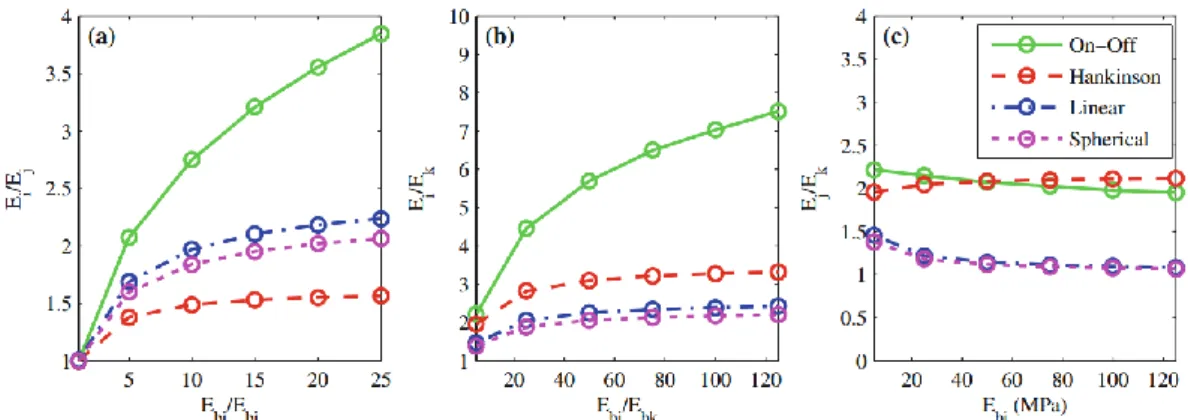
parameters on the output degree of anisotropy is investigated in the following. The same simulations as described previously were run again with 5 different degrees of anisotropy. Simulation parameters used and corresponding results are shown in Table 5. Ebj and Ebk are maintained constant, respectively equal to 5
MPa and 1 MPa while Ebi varies between 5 MPa and 125 MPa in order to increase
the input degrees of anisotropy of the model. As a consequence, both input ratios Ebi/Ebj and Ebi/Ebk are affected. The first ratio varies between 1 and 25 while the
second varies from 5 to 125. Fig. 8a displays the evolution of the degree of anisotropy of the modelled domain Ei/Ej according to the input ratio of stiffness in
its beams Ebi/Ebj and Fig. 8b displays the evolution of the degree of anisotropy of
the modelled domain Ei/Ek according to the input ratio of stiffness in its beams
Ebi/Ebk. Fig. 8c presents the evolution of the third degree of anisotropy Ej/Ek
Table 5
Input degree of anisotropy applied to the beams and output degree of anisotropy of the domain measured according to the method of orthotropic generation
Ebi/Ebj 1 5 10 15 20 25 Ei/Ej (Regular arrangement) 1.00 5.00 10.00 15.00 20.00 25.00 Ei/Ej (On-Off) 1.00 2.07 2.75 3.21 3.56 3.85 Ei/Ej (Hankinson) 1.00 1.38 1.49 1.53 1.55 1.57 Ei/Ej (Linear) 1.01 1.69 1.97 2.10 2.18 2.24 Ei/Ej (Spherical) 1.00 1.60 1.84 1.95 2.02 2.06 Ebi/Ebk 5 25 50 75 100 125 Ei/Ek (Regular arrangement) 5 25 50 75 100 125 Ei/Ek (On-Off) 2.22 4.46 5.69 6.49 7.03 7.51 Ei/Ek (Hankinson) 1.96 2.82 3.10 3.21 3.27 3.31 Ei/Ek (Linear) 1.47 2.05 2.25 2.34 2.39 2.42 Ei/Ek (Spherical) 1.38 1.89 2.05 2.13 2.17 2.20
For every law, as the input degree of anisotropy is higher, the output degree of anisotropy of the domain increases, but as it grows slower than the input. 3.2. Off-axis behavior
Domain’s effective Young’s modulus is measured every 10°-step and the results are plotted on Fig. 9 from Ej to Ei. Each law displays a different evolution. In the
following, ΔE is defined as the amplitude between E(0°) and E(90°): ΔE = E(0°) - E(90°). The effective Young’s modulus of an α-rotated domain E(α) decreases very fast in the case of regular domains. E(α) has already decreased of 93% of ΔE when α reaches 40°. Afterwards, the effective Young modulus slowly decreases until E(90°). At the contrary, using either on-off, Hankinson’s, linear and spherical laws, the switch between E(0°) and E(90°) is smoother.
Results obtain with the 4 different laws are compared with results obtain with the Hankinson’s equation as reference. The use of Hankinson’s equation was proven efficient to represent mechanical properties evolution along fiber angle in strongly anisotropic material, including Young modulus [25, 26].
Considering measured E(0°) and E(90°) are corrects, theoretical 𝐸𝑡ℎ(10°) to 𝐸𝑡ℎ(80°) are calculated with Hankinson’s equation from E(0°) and E(90°):
Eth(α) = E(0°)∙sin E(0°)∙ E(90°)2α+ E(90°)∙cos2α. (11)
Theoretical and mean measured effective Young’s Modulus are then compared. The indicator used to evaluate methods efficiency toward continuum mechanics is the Normalized Root Mean Squared Error (12):
𝑁𝑅𝑀𝑆𝐸 = √∑ (𝐸(α)−𝐸𝑡ℎ(α)) 2 80°
10°
𝑛∙(max(𝐸(α))−min(𝐸(α))), (12)
where n is the number of summed quantities (8 for 10 °-steps). The NRMSE allows to compute a mean error between the measured and the estimated off-axis Young’s moduli normalized by the range of the measured Young’s moduli. The lower the NRMSE, the more accurate the chosen law. The resulting NRMSE for the 5 studied cases are displayed in Table 6.
Table 6
NRMSE values calculated for the different method of orthotropic generation
Law NRMSE calculated
Regular arrangement 0.579
On-off 0.164
Hank 0.288
Linear 0.326
Spherical 0.390
The lowest NRMSE is shown by the On-off interpolation method: 0.164.
Hankinson’s law comes second. Linear and spherical law’s NRMSE is higher and regular arrangement NRMSE is the highest and equals 0.579.
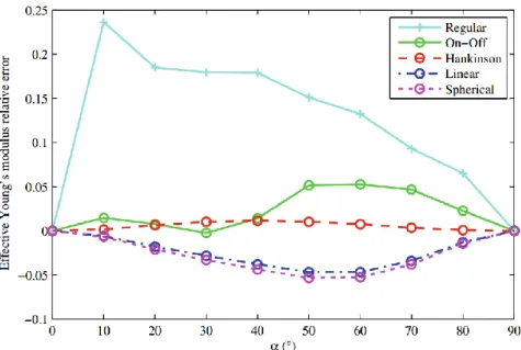
To allow more detailed analysis, the relative error (13) evolution toward every 10°-steps rotation angle is also calculated:
𝑅𝑒𝑙𝑎𝑡𝑖𝑣𝑒𝑒𝑟𝑟𝑜𝑟(𝛼) =𝐸(𝛼)−𝐸𝑡ℎ(𝛼)
𝐸𝑡ℎ(𝛼) . (13) The results according to the law chosen are displayed Fig. 10.
The relative error between effective Young’s modulus of the regular domain and Hankinson’s equation increases with specimen angle (α) until it reaches its maximum between 0° and 20° rotation (the measurement resolution is not small enough to give more precision in the estimation). Once this maximum is reached, the error seems to decrease linearly until a 90° rotation. As hinted by NRMSE, relative errors are lower in the case of packed domains, whatever the rotation
angle and the law chosen is. However, unlike NRMSE suggested, On-Off interpolation errors are higher than Hankinson’s interpolation relative errors, unless for 30°. For 20° and 40°, On-Off error is as low as Hankinson’s error, but the low 30° “On-off” errors compensate 10° and larger angle than 50° error. Indeed, for larger angles, the Young’s Modulus decreased enough for the squared error to be also very small once normalized. Linear and Spherical laws errors increases with α until it reaches a maximum of between 50° (approximately 5.33%) and 60° (approximately 5.28%). Then it decreases when α tends to 90°.
4. Discussion
4.1 Degrees of anisotropy
When focusing on two main directions of the considered orthotropic material, degrees of anisotropy of the global domain obtained using regular cubic domains equal to the input anisotropy ratio of the beam Young’s Moduli. However, for packed domains, the global domain degree of anisotropy measured is always lower than the input. Moreover the output degree of anisotropy tends to reach an asymptote. Increasing significantly the input ratio does not affect significantly the domain anisotropy anymore. The value of the asymptotes varies depending on the Young’s Modulus computation law chosen. This value is also affected by the stiffness of the bond in the third main direction (see Fig. 8c). Because of the previous phenomenon, it is impossible to obtain a high degree of anisotropy if the domain is packed with the Young’s moduli calculation strategy tested.
Having very large differences between beams elastic properties to obtain a given global structure degree of anisotropy leads to two consequences. On one hand it increases the computational time as the time constant between two computational increments is directly related to the highest beam stiffness of the domain. Thus, to simulate a phenomenon lasting a given time, a simulation using packed domain instead of regular domain will last longer. On the other hand it can also lead to unphysical local effects leading to easy buckling of the structure because beams with extremely different Young’s Modulus interact with each other.
4.2 Off-axis effective Young’s moduli
Cubic regular arrangement present the exact degrees of anisotropy in the main directions of orthotropy but the effective modulus of the structure when loaded off the main directions is inaccurate compared to packed domains. Indeed, the relative error varies between 6% and 24% depending on the angle formed by the load and the main direction of orthotropy in the case of regular domains. The effective Young’s modulus is over-estimated by this law. For a small angle, the relative error between the effective modulus and the theoretical modulus calculated can be ten times smaller for packed domains. In those last types of domains, the relative error, whatever the chosen law is, between effective modulus and its theoretical value is always lower than 5.4%. The most consistent law is Hankinson’s
equation, while on-off law displays very good results as well. Linear and spherical laws present slightly larger relative errors and tend to under-estimate the effective Young’s modulus, especially around 50° to 70° rotation toward one main
direction. Thus, as soon as the model is used for complex geometry, load state, displacement or strain fields, this last strategy of model arrangement becomes way more relevant than regular arrangement-based models (in the case of low degree of anisotropy).
5. Conclusions
To model orthotropic media at mesoscopic or macroscopic scale, with DEM, by the way of Euler-Bernoulli beams, the two proposed approaches led to two different behaviors. Regular cubic arrangement displays perfect stiffness in its main directions of orthotropy, but its response is not as good when loaded off-axis. It suffered up to 24% relative error with Hankinson’s equation. In the case of packed domains, four laws to establish beams Young’s modulus were evaluated. Unlike cubic regular arrangements, it was not possible to reach a significantly high degree of orthotropy with any of these four laws. However, in every case their off-axis behavior was very good leading only to 7% relative error in the worst tested scenario. On-off law, even if very simple, seemed to present a good compromise between reachable anisotropy which was the highest of the four laws and off axis behavior which was the second best fitting with Hankinson’s
equation. Thus, the applications of the two approaches are distinct. Regular domains are mandatory when modeling materials with anisotropy degree is high
(starting approximately from 10); but, in the case of low anisotropy, packed domains are preferable due to their advantage in off-axis behavior. For very small degrees of anisotropy (approximately up to 2) Hankinson’s law would be the privileged choice. For higher anisotropy (between 2 and 8), On-off law becomes the optimized alternative. Linear and Spherical does not bring competitive benefits towards the two previous laws.
This last approach might be improved in order to increase their reachable orthotropy degree. For instance, the use of Timoshenko beams instead of Euler-Bernoulli model, adding shear deflection to the bonds would be an interesting possibility to investigate. Exploring new laws to determine beams Young’s Modulus might also be a path to follow in order to both reach larger degrees of anisotropy and better off-axis behavior. Every tested law but “On-off” was monotonic, to go further, experimenting nonmonotonic laws may perhaps be a solution to rise up the asymptotic anisotropy degree reachable. In the case of either Euler-Bernoulli or Timoshenko beams, adapting the beams section could be one more solution to increase the domains anisotropy as it would change the ratio between tensile and bending potential energy of the system. In this last case, extra attention should be focused on the interaction between beam Young’s moduli and sections since both those variables impact the structure global stiffness.
Acknowledgement
The authors would like to acknowledge GranOO staff members, especially Jean-Luc Charles and Damien André for the training they provided.
Compliance with Ethical Standards:
Conflict of Interest: The authors declare that they have no conflict of interest.
Funding: These works were conducted thanks to the support of the region Bourgogne Franche-Comté and were funded by the ANR-10-EQPX-16 XYLOFOREST-XYLOMAT and the French MESRI.
References
[1] André D, Iordanoff I, Charles JL, Néauport J (2012) Discrete element method to simulate continuous material by using the cohesive beam model. Comput. Methods Appl. Mech. Eng. 213– 216:113–125
https://doi.org/10.1016/j.cma.2011.12.002
[2] Jauffrès D, Martin CL, Lichtner A, Bordia RK (2012) Simulation of the elastic properties of porous ceramics with realistic microstructure, Model. Simul. Mater. Sci. Eng. 20 :045009.
https://doi.org/10.1088/0965-0393/20/4/045009
[3] Jefferson G, Haritos GK, McMeeking RM (2002) The elastic response of a cohesive
aggregate—a discrete element model with coupled particle interaction. J. Mech. Phys. Solids. 50:2539–2575
https://doi.org/10.1016/S0022-5096(02)00051-0
[4] Potyondy DO, Cundall PA (2004) A bonded-particle model for rock, Int. J. Rock Mech.
Min. Sci. 41:1329–1364
https://doi.org/10.1016/j.ijrmms.2004.09.011
[5] Swope WC, Andersen HC, Berens PH, Wilson KR (1982) A computer simulation method
for the calculation of equilibrium constants for the formation of physical clusters of molecules: Application to small water clusters. J. Chem. Phys. 76:637–649
https://doi.org/10.1063/1.442716
[6] Levitt M, Warshel A (1975) Computer simulation of protein folding. Nature. 253:694–
698
https://doi.org/10.1038/253694a0
[7] Cundall PA, Strack OD (1979) A discrete numerical model for granular assemblies.
Geotechnique 29:47–65
https://doi.org/10.1680/geot.1979.29.1.47
[8] André D (2012) Modélisation par éléments discrets des phases d'ébauche et de doucissage de la silice. Université de Bordeaux. (in French)
[9] Hentz S, Donzé FV, Daudeville L (2004) Discrete element modelling of concrete
submitted to dynamic loading at high strain rates. Comput. Struct. 82:2509–2524
https://doi.org/10.1016/j.compstruc.2004.05.016
[10] Leclerc W (2017) Discrete element method to simulate the elastic behavior of 3D heterogeneous continuous media. Int. J. Solids Struct. 121:86–102
https://doi.org/10.1016/j.ijsolstr.2017.05.018
[11] Leclerc W, Haddad H, Guessasma M (2017) On the suitability of a Discrete Element
Method to simulate cracks initiation and propagation in heterogeneous media. Int. J. Solids Struct. 108:98–114.
https://doi.org/10.1016/j.ijsolstr.2016.11.015
[12] Iliev PS, Wittel FK, Herrmann HJ (2018) Discrete element modeling of free-standing wire-reinforced jammed granular columns. Comp. Part. Mech.
[13] Espinosa C, Lachaud F, Limido J, Lacome JL, Bisson A, Charlotte M (2015) Coupling continuous damage and debris fragmentation for energy absorption prediction by cfrp structures during crushing. Comp. Part. Mech. 2:1-17
https://doi.org/10.1007/s40571-014-0031-6
[14] Eberhard P, Gaugele T (2013) Simulation of cutting processes using mesh-free Lagrangian particle methods. Comput. Mech. 51:261–278
https://doi.org/10.1007/s00466-012-0720-z
[15] Iliescu D, Gehin D, Iordanoff I, Girot F, Gutiérrez ME (2010) A discrete element method for the simulation of CFRP cutting, Compos. Sci. Technol. 70:73–80
https://doi.org/10.1016/j.compscitech.2009.09.007
[16] Pfeiffer R, Lorong P, Ranc N (2015) Simulation of green wood milling with discrete element method. in: Proc. 22nd Int. Wood Mach. Semin. IWMS 2015:57–72
[17] Roux A, Laporte S, Lecompte J, Gras LL, Iordanoff I (2016) Influence of muscle-tendon complex geometrical parameters on modeling passive stretch behavior with the Discrete Element Method. J. Biomech. 49:252–258
https://doi.org/10.1016/j.jbiomech.2015.12.006
[18] Duan K, Kwok CY, Pierce M (2016) Discrete element method modeling of inherently
anisotropic rocks under uniaxial compression loading. Int. J. Numer. Anal. Methods Geomech. 40:1150–1183
https://doi.org/10.1002/nag.2476
[19] Lochmann K, Oger L, Stoyan D (2006) Statistical analysis of random sphere packings
with variable radius distribution. Solid State Sci. 8:1397–1413
https://doi.org/10.1016/j.solidstatesciences.2006.07.011
[20] B.D. Le, F. Dau, J.L. Charles, I. Iordanoff (2016) Modeling damages and cracks growth in composite with a 3D discrete element method, Compos. Part B Eng. 91:615–630
https://doi.org/10.1016/j.compositesb.2016.01.021
[21] Maheo L, Dau F, André D, Charles JL, Iordanoff I (2015) A promising way to model
cracks in composite using Discrete Element Method. Compos. Part B Eng. 71:193–202
https://doi.org/10.1016/j.compositesb.2014.11.032
[22] Hankinson RL (1921) Investigation of crushing strength of spruce at varying angles of grain, Air Serv. Inf. Circ. 3:130
[23] Cramer SM, McDonald KA (1989) Predicting lumber tensile stiffness and strength with
local grain angle measurements and failure analysis. Wood Fiber Sci. J. Soc. Wood Sci. Technol. USA
[24] Kenney JF (2013) Mathematics of Statistics, Literary Licensing, LLC.
[25] Radcliffe BM (1965) A theoretical evaluation of Hankinson's formula for modulus of elasticity of wood at an angle to the grain. Quart Bull Mich. Agr Exp Sta. 48:286–295 [26] Yoshihara H (2009) Prediction of the off-axis stress-strain relation of wood under compression loading. Eur. J. Wood Wood Prod. 67:183–188
Figures
Fig. 1. Regular arrangement whose principal directions are 𝑖,⃗ 𝑗 and 𝑘⃗
Fig. 3. Scheme of the angles used in off-axis Young’s modulus computation. θ is the polar angle
and φ is the complementary azimuthal angle in the frame (𝑗,⃗⃗⃗⃗ 𝑘⃗ , 𝑖)⃗⃗
Fig. 5. Left: regular cubic arrangement between numerical compression plates – Right: random
sphere packing arrangement in the same configuration
Fig. 6. Left: regular domain rotated by 20° between compression plates, right: packed domain in
the same configuration
Fig. 7. Degrees of anisotropy measured according to the method of orthotropy generation and
Fig. 8. Domain anisotropy degrees evolution according to input ratio between longitudinal and
transversal beams stiffnesses
Fig. 9. Off-axis effective Young’s modulus measured by numerical compression experiments for
Fig. 10. Relative Error between the effective Young’s modulus ratio measure and estimated for