Science Arts & Métiers (SAM)
is an open access repository that collects the work of Arts et Métiers Institute of
Technology researchers and makes it freely available over the web where possible.
This is an author-deposited version published in: https://sam.ensam.eu
Handle ID: .http://hdl.handle.net/10985/11176
To cite this version :
Christophe GIRAUDAUDINE, Frédéric GIRAUD, Michel AMBERG, Betty LEMAIRESEMAIL -Generalized modal analysis for closed-loop piezoelectric devices - Smart materials and structures - Vol. 24, n°8, p.085028 (10pp) - 2015
Any correspondence concerning this service should be sent to the repository Administrator : archiveouverte@ensam.eu
Generalized modal analysis for closed-loop
piezoelectric devices
Christophe Giraud-Audine
1,2, Frédéric Giraud
2,3, Michel Amberg
2,3and
Betty Lemaire-Semail
2,31
Arts et Métiers Paristech, Lille, 59046 France
2L2EP—IRCICA 50 rue de Halley, Villeneuve d’Ascq, 59650 France 3Université Lille 1, Villeneuve d’Ascq, 59655 France
E-mail:christophe.giraud-audine@ensam.eu
Abstract
Stress in a piezoelectric material can be controlled by imposing an electricalfield. Thanks to feedback, this electricalfield can be a function of some strain-related measurement so as to confer on the piezoelectric device a closed-loop macroscopic behaviour. In this paper we address the modelling of such a system by extending the modal decomposition methods to account for the closed loop. To do so, the boundary conditions are modified to include the electrical feedback circuit, hence allowing a closed-loop modal analysis. A case study is used to illustrate the theory and to validate it. The main advantage of the method is that design issues such as the coupling factor of the device and closed-loop stability are simultaneously captured.
Keywords: piezoelectric, feedback, modal analysis
(Somefigures may appear in colour only in the online journal) 1. Introduction
Piezoelectric devices are intrinsically suited for closed-loop structure due to their reversibility: they can be actuators and sensors. It is therefore sensible to modify the dynamics of such a device by feeding back the strain state using the direct piezoelectric effect. Then, applying a voltage depending on this measured strain state, it is possible for instance to confer a modified compliance to the system or increase dissipation in an assigned frequency band. This is the basic idea in many applications where frequency control or damping is required, especially in the case of collocated structures.
In Moheimani et al (2003) or Fairbairn and Mohei-mani (2013), for instance, a feedback model is used to modify the damping of structures with different strategies. As a pre-requisite to apply the methods though, the frequency response of the mechanical structure must be identified. Preumont et al (2008) address the problem of controlling the vibrations of large trusses. A quasi-static model of the actuator was con-sidered, because in this case the dynamics of the piezoelectric actuator was much faster than that of the controlled structure. This assumption cannot hold in some cases, e.g. MEMS or energy harvesters. Indeed, in this latter case, the overall
dynamics must be accounted for since the resonance is the key issue (Dutoit et al2005, Lavrik et al2004). Moreover, it is also a well known fact that the coupling factor is inherent to the overall feedback structure and the design of the actuator (Preumont 2005). Therefore, the designer should consider a comprehensive approach in order to take into account the dynamics of the piezoelectric actuator in the case of the closed-loop structure. Of course, the model is crucial in this context.
The literature on the subject of piezoelectric actuator modelling is abundant, concentrating on fine quasistatic modelling (Smits and Choi 1991, Goldfarb and Cela-novic 1997) or dynamic operation near a specific resonance (Mason 1935, Ballas 2007). When addressing broadband operations, one has to consider several modes (Meir-ovitch 2003). Therefore, modal decomposition is a natural and widely used tool (Erturk and Inman 2009, Ducarne et al 2012). The approach consists in finding the modal shapes for a given electrical condition (open circuit or short circuit, the latter being the most used) where the electricfield or charge can be eliminated. These modal shapes are used to form a orthonormal basis on which any response can be decomposed (Meirovitch 2003, Geradin and Rixen 2014).
Moreover, in some cases, the modal shapes have analytical expressions that are helpful to deduce design rules (Ducarne et al2012). Even for more complex geometry, modal shapes of known simpler structures can be used to model the dynamics (Erturk2012). However, since the initial analysis is performed in open loop, many modes may be necessary to model the closed-loop response since the resonant frequencies may be modified. Thus, insight can be lost, and in practice the accuracy of the design is dependent on the number of modes that are considered.
In this paper, we show that the modal analysis method can be generalized to take into account the closed loop. The remainder of the paper is as follows. Section 2 recalls the modelling of a clamped–free beam equipped with a sensor to provide feedback possibilities. Section 3 introduces the extension of the modal analysis in a closed loop. We show that the boundary conditions can be modified to incorporate the effect of the feedback as moments dependent on the measurement. By properly dividing the contribution of the feedback-induced moment into dissipative or generative (active power) and non-dissipative (reactive power) con-tributions, we prove that modal projection on a closed-loop modal basis is possible. Section 4 presents experimental results to illustrate the approach and validate the prediction of a model based on the theory developed.
2. Modal analysis of a bender
2.1. Assumptions and notation
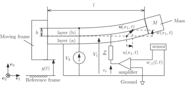
The schematic diagram offigure1depicts a simplified model of a slender beam used in this paper. The bender is mechanically excited at one end, and feedback is used to modify its dynamic behaviour. In the following, the overall feedback circuit will be modelled as an amplifier and a series impedance so as to take into account simplefiltering circuits. Regarding the mechanical modelling, the problem is supposed to be two dimensional in the sense that the different fields are not dependent on x2. The bender is constituted by
two piezoelectric layers polarized to operate on a 31 coupling. The end at x1=0 is clamped to the moving frame, while a proof mass M is clamped at the free end at x1= . Thel
moving frame is translated along the direction e3; its position
relative to the reference frame is y(t). The bender is supposed to be mechanically unloaded, apart from the effect of inertia.
The electrodes are connected as shown. In practice, as will be explained later, the voltage V2 is fixed while the
voltage V1is varied. We consider small displacements, and
since the electrodes impose equipotentials it will also be assumed that the electrical field is mainly along the e3
direction. In the following, the voltage V t1( )is generated from the measure of the free tip of the bender w,1( , )L t.
Voigt notation for tensors will be used in this paper. x⊤is
the transpose of vector x. Matrices will be indicated by brackets, e.g., c[ E] is the matrix of compliances at fixed electricalfield. f,ijdenotes the partial derivative with respect to space variables xi and xj; a repeated index denotes a
repeated partial derivative with respect to one of the space variables. Finally f˙ denotes the time derivative of the func-tion f.
2.2. Model
2.2.1. Piezoelectric law. For the following discussion, it is convenient to consider displacement and voltage to formulate the problem, thus the relevant piezoelectric equations used throughout this paper are (Ikeda1996)
c e e T S E D S E [ ] [ ] [ ] [ ] (1) E t S ⎪ ⎧ ⎨ ⎩ ϵ = − = +
with e[ ] the piezoelectric coefficient matrix and [ ]ϵS the
permittivity matrix at fixed strain. T, S are the stress and strain tensors; E, D are the electric and electrical displacement fields. The corresponding thermodynamic potential is then written as (Tiersten1969)
G S E T S D E
d 2( , )= d − d . (2)
2.2.2. Kinematics of the model. The bonding of the layers is supposed to be perfect, thus a continuous displacementfield is considered. In this study shear strains are not considered, the bender being thin and the frequencies being low. Thus an Euler–Bernoulli displacement field is used, given by (Weaver et al1990, Geradin and Rixen2014)
x x t u x x t u x t x w x t u x x t u x x t w x t y t u( , , ) ( , , ) ( , ) ( , ) ( , , ) 0 ( , , ) ( , ) ( ) (3) 1 3 1 1 3 1 3 ,1 1 2 1 3 3 1 3 1 ⎧ ⎨ ⎪ ⎩⎪ = = − = = +
which results in the strainfield
{
u x t x w x t}
S= ,1( , )1 − 3 ,1( , ), 0, 0, 0, 0, 01 . (4)
⊤
2.2.3. Electrostatic solution. Considering the electrical displacement D, the condition divD=0 must hold. It is assumed that the layers are thin along e3 compared to the
dimensions in the other directions. Moreover, the potentials are imposed on the electrodes located on the horizontal sides of the bender, hence it is assumed that E3≫E1and E3≫E2.
Let d∈{ , }a b denote the considered sub-domain relative to the layers, then for each layer the electric field is given by
E= −grad(ϕd). Using (4) and (1), and neglecting the influence of the electric field along e1and e2, this condition
reduces to:
Dd3,3=0⇔ −e w31 ,1( , )x t1 −ε ϕ33 d( ,x x1 3, )t ,33=0. (5) Integrating twice with respect to x3gives the expression of the
electrical potential ϕd in one layer of the bender, which should be written as (Nadal et al2014)
x x t e w x t x A x t x B x t ( , , ) ( , ) 2 ( , ) ( , ). (6) d 1 3 S d d 31 33 ,11 1 3 2 1 3 1 ϕ ϵ = − + +
The functions A x td( , )1 , B x td( , )1 are functions to be
determined from the equipotential conditions at the electro-des: (7) h V V h V layer (a) ( ) 0 (0) layer (b) (0) ( ) . a a 1 b 1 b 2 ϕ ϕ ϕ ϕ − = = = =
2.2.4. Dynamic equations. The augmented Lagrangian of the piezoelectric energy harvester is given by
x x t x x t G x x t M l t l t V Q V Q Fy u u u u 1 2 ˙ ( , , ) ˙ ( , , ) ( , , )d 1 2 ˙ ( , 0, ) ˙ ( , 0, ) (8) 1 3 1 3 2 1 3 1 1 2 2 =
∭
ρ − Ω + + + + ⊤ ⊤where the last four contributions correspond respectively to the kinetic energy of the proof mass M, the energy supplied by the two generators, and the mechanical energy due to the external force applied for the mechanical excitation.
Applying variational calculus to the Lagrangian (8) leads to the equations of the problem (Hammond 1981). The internal mechanical equilibrium involves the following equations for the extension and the flexion displacement field respectively: u x t¨ ( , )1 u,11( , )x t1 0 (9 )a − + =
(
w x t y x t)
w x t w x t b ¨ ( , ) ¨ ( , ) ¨ ( , ) ( , ) 0 (9 ) 1 1 ,11 1 ,1111 1 − + + − = where• is the mass per unit length
• is the rotational inertia per unit length • is the compressive rigidity
• is the equivalent flexion rigidity.
The mechanical boundary conditions at the free end are
u,1( , )l t exV t2( ) (10 )a = − w ( , )l t V V b 2 (10 ) fl ,11 1 2 ⎜ ⎟ ⎛ ⎝ ⎞ ⎠ = − w,111( , )l t w¨ ( , ),1 l t Mw l t¨ ( , ) My t¨ ( ) (10 )c − = +
where the electromechanical conversion coefficients for extension and bending are respectively
e a (11 )a ex 31 = e ah. (11 )b fl 31 =
At the other end of the bender, the displacements are supposed to be perfectly imposed, hence
u(0, )t =0 (12 )a w(0, )t =0 (12 )b w,1(0, )t =0. (12 )c
The electrical charges can be deduced from
(
)
Q t1( ) S 2V1 V2 fl w,1( , )x t l (13 )a 0 ⎡⎣ ⎤⎦ = − − Q t Q t V u x t b 2 ( ) ( ) S [ ( , )]l (13 ) 2 + 1 = 2−ex 0 al h c with S . (13 ) S 33 = ϵ S is the clamped capacitance.
3. Theoretical study
The study will consider the case when V2is constant, which is
necessary in practice to apply a compressive prestress in order to avoid excessive tensile stress during bending. Therefore, the displacementfield u x t( , ) is static since the extension and flexion fields are decoupled, as can be deduced from the previous equations. Besides, without loss of generality, the frequency range considered is supposed to be sufficiently low to neglect the rotational inertia effects in (9b) and thus they will not be considered.
The equilibrium (9b) with the boundary conditions (10b), (10c), (12b) and (12c) are used for the modal analysis of the bender. To do so, the system is supposed to be free, hence all independent sources of the system are cancelled. This implies that, for the mechanical side, y(t) must be set to zero.
At a considered resonant angular frequencyω, the solu-tion to (9b) is
w x t( , )1 =ψ( ) ( )x1 η t (14) where ψ( )x1 is the modal shape written as a linear
combination of the Duncan functions (see appendixA),
x A x l B x l C x l D x l ( ) s c s c (15) 1 1 1 1 1 2 1 2 1 ⎜ ⎟ ⎜ ⎟ ⎜ ⎟ ⎜ ⎟ ⎡ ⎣⎢ ⎛ ⎝ ⎞⎠ ⎛⎝ ⎞⎠ ⎛⎝ ⎞⎠ ⎛⎝ ⎞⎠ ⎤ ⎦⎥ ψ = β + β + β + β
and η( )t is the vibration,
t t
( ) sin( ). (16)
η =η ω +α
Moreover the dispersion condition is
l 0. (17)
4 2 4
β −ω =
The problem can be simplified further thanks to (12b) and (12c):
A=B=0.
We proceed in the following by modifying the boundary condition (10b) to include the feedback effect.
3.1. Electrical equations
The electrical circuit that filters and amplifies the measure-ment signal is now introduced. Assuming a linear circuit, a Thévenin equivalent circuit is considered. We restrict the study to the case when the voltage source is proportional to the measured signal4:
v tc( )=G w l tc ( , ) (18) where Gc is the sensor gain possibly followed by an
amplification. For the purpose of the study, we substitute
V1= V22 + vin (10b) and (13a). This reflects the fact that the
bending moment is actually controlled by disturbing the middle plane voltage from the value it would normally have in a pure extension case. Since in the following harmonic oscillation will be studied, the various variables are expressed using complex vectors. Then, the displacement w x t( , )1 is
written5
w x t( , ) w x t( , ) ( ) ( )x t ( ) ex t
1 → 1 =ψ 1 η =ψ 1 η jω
with η=ηejα. Furthermore, equations will be written in a rotating frame so that the ejωt can be dropped, and for
shorthand W,1 ...=ψ,1 ...( )L η.
Let Z = NP(j )(j )ωω be the equivalent series impedance of the Thévenin equivalent generator; the equations of the circuit are
i v v Z (19 )a c = − v i W b j S j . (19 ) fl ,1 ω = + ω
The second equation is deduced by time derivation of (13a). According to (13a) and (10b), v and vc can be expressed
in terms of displacement or derivatives of displacement. Writing P(j )ω = ∑pk(j )ωk and N(j ) n (j )
k k
ω = ∑ ω
k ∈ , equations (+ 19a), (19b) and (10b) can be combined, resulting in the following equation:
(20) p n W p W G n w W (j ) (j ) (j ) (j ) 0. k P S k k k N k k k P k k k N k k 0 deg( ) 1 0 deg( ) ,11 fl2 0 deg( ) 1 ,1 fl c 0 deg( ) ⎡ ⎣ ⎢ ⎢ ⎤ ⎦ ⎥ ⎥
∑
∑
∑
∑
ω ω ω + + − = = + = = + =For the sake of clarity, the condition n0≠0 is assumed. In this case, the previous result can be reformulated as
W,11 R(j )W,11 S(j )W,1 T(j )W (21) = ω + ω + ω where R (j ) (j ) (j ) k P p n k k N n n k 0 deg( ) 1 1 deg( ) s k k 0 0
∑
∑
ω = − ω − ω = + = , S(j ) nfl2P(j ) 0 ω = − ω and T(j ) nflN(j ) 0 ω = ω are polynomials. This defines the new boundary condition for the bendingmoment including the closed loop. For the following discussion, rewrite the previous equation:
(
)
W R W S W T W R W S W T W (j ) (j ) (j ) j (j ) (j ) (j ) (22) d d d q q q ,11 ,11 ,1 ,11 ,1 ω ω ω ω ω ω ω = + + + + +where R (j )d ω , R (j )q ω , Sd(j )ω , S (j )q ω , Td(j )ω and T (j )q ω are
real even polynomials of ω. Only the non-dissipative contribution of this condition must be considered for modal analysis. Multiplying both sides of (20) by the conjugate of the rotation speed at the end of the tip (jωW,1)* gives the complex power transmitted to the bender by the feedback:
W W R W S W T W W j j (j ) (j ) (j ) . ,11 ,1* ,11 ,1 ,1* ⎡⎣ ⎤⎦ ω ω ω ω ω − = − + +
Two different contributions should be distinguished: • imaginary terms, corresponding to real projection on the
real axis of the closed-loop bending moment complex vector (therefore leading or lagging in quadrature with the rotation speed), which are conservative;
• real terms, corresponding to imaginary part of the closed-loop bending moment complex vector, which are either dissipative or supplying power.
Since W , W,1and W,11are in phase, it can be concluded that
real parts of R, S and T (denoted Rd, Sd and Td in the
following) will contribute to the reactive power, while imaginary parts (denoted Rq, Sq, Tq) will be responsible for
active power.
3.2. Secular equation
For the modal analysis, only the conservative contribution of the system need be considered. Thus, according to the pre-vious discussion, only Rd, Sd and Td are relevant, and thus,
after cancelling the η that appear on both sides of the equality sign, the boundary conditions (10b) and (10c) are rewritten as
l R l S l T l a ( ) d( ) ( ) d( ) ( ) d( ) ( ) (23 ) ,11 ,11 ,1 ψ = ω ψ + ω ψ + ω ψ l M l b ( ) ( ) (23 ) ,111 2 ψ = − ω ψ
Using (17) to rewrite these conditions inβ, a general secular equation can be obtained (see appendixB).
Solving this equation for β=βk gives the resonant fre-quenciesωk using (17), and once replaced in (14) the mode
shapeψ can be obtained up to a multiplicative constant. Ink
the usual modal analysis method, the modes are used to decompose the solution to a given excitation. These mode shapes, which already partly include the electrical feedback, are now compared to the classical mode shapes that would arise from considering short-circuit conditions.
3.3. Properties of the closed-loop modal shapes
The closed-loop (CL) modal shapes can be used to describe the solution to the forced vibration problem. Indeed, letθj( )x1
be the normalized open-loop (OL) modal shapes of the
4
A more general case involves a frequency-dependent measurement voltage. However, since there are no fundamental differences in the outline of the demonstration, this simpler case is considered.
5
bender, obtained by replacing the feedback circuit by a short circuit, which fulfil
0 (24) j j j 2 2 ,1111 ν θ θ − + =
where νk are the corresponding modal angular frequencies,
for the boundary conditions
(0) 0 (25) j θ = (0) 0 (26) j,1 θ = l ( ) 0 (27) j,11 θ = l M l ( ) ( ). (28) j,111 j2 θ = − ν θ
The normalization considered is defined by (Erturk and Inman2009) x x M l ( )d ( ) 1. (29) l j j 0 2 1 1 2
∫
θ + θ =Note that the same normalization will be applied to theψ .k
The OL modal shapes fulfil
x x x M ( ) ( )d (30) l j k k j jk 0 1 1 1
∫
θ θ + θ θ =δwhereδjk=1if j = k andδjk= 0if j≠ . Therefore, the CLk
modal shapesψk( )x1 can be expressed as
x x ( ) ( ) . (31) k j kj j kj 1 1 1
∑
ψ = α θ α ∈ = ∞ Since theψk( )x1 depend on the wave numbers {β , whichk}
form an increasing sequence, it is clear from the expression (15) that
x x k j
( ) ( ) if . (32)
k 1 j 1
ψ ≠ψ ≠
It follows that the ψ are independent vectors that can bek
related to a free basis, and thus can also be used as a basis; that is, any response of the bender can be written
w x t( , ) ( )x ( ).t (33) k k k 1 1 1
∑
ψ η = = ∞The standard procedure to solve the vibration problem involves the projection of the dynamic equilibrium verified by a modal shapeψ on a modal shapek ψj:
x t x t t x ( ) ¨ ( ) ( ) ( ) ( )d 0. (34) l k k k k j 0 ⎡⎣ 1 ,1111 1 ⎤⎦ 1
∫
ψ η + ψ η ψ =Using integration by parts, and the boundary conditions (23a) and (23b), the previous equation for harmonic vibrations (i.e.
t t ¨ ( )k k k( ) 2 η = −ω η ) is rewritten as follows: x x x M l l R l S l T l l x x x ( ) ( )d ( ) ( ) ( ) ( ) ( ) ( ) ( ) ( ) ( ) ( ) ( )d 0. (35) k l k j k j d k k d k k d k k j l k j 2 0 1 1 1 ,11 ,1 ,1 0 ,11 1 ,11 1 1 ⎛ ⎝ ⎜ ⎞⎠⎟ ⎡⎣ ⎤⎦
∫
∫
ω ψ ψ ψ ψ ω ψ ω ψ ω ψ ψ ψ ψ − + − + + + =Considering the special case where j = k, and using the proposed normalization given by (29), the potential energy for the modal shape, including the feedback, fulfils
R l S l T l l x x ( ) ( ) ( ) ( ) ( ) ( ) ( ) ( ) d . (36) d j j d j j d j j j l j j ,11 ,1 ,1 0 ,11 1 2 1 2 ⎡ ⎣ ⎤⎦
∫
ω ψ ω ψ ω ψ ψ ψ ω − + + + =The projection of the dynamic equilibrium of modeψjon mode
k
ψ leads to an equation similar to (35) where the k and j indexes are swapped. The difference of these equations would give
(
)
x x x M l l R l S l T l l R l S l T l l ( ) ( )d ( ) ( ) ( ) ( ) ( ) ( ) ( ) ( ) ( ) ( ) ( ) ( ) ( ) ( ) ( ) ( ) 0. (37) j k l k j k j d j j d j j d j j k d k k d k k d k k j 2 2 0 1 1 1 ,11 ,1 ,1 ,11 ,1 ,1 ⎛ ⎝ ⎜ ⎞ ⎠ ⎟ ⎡ ⎣ ⎤ ⎦ ⎡⎣ ⎤ ⎦ ∫
ω ω ψ ψ ψ ψ ω ψ ω ψ ω ψ ψ ω ψ ω ψ ω ψ ψ − + + + + − + + =Therefore, the CL modal shapes are generally not orthogonal in CL for the functional (34).6Actually, in CL the functional should be modified to account for the electrical equilibrium of the bender and the circuit. Fortunately, this tedious task can be avoided to solve the forced response due to the feature discussed below.
3.3.1. Response to the forced vibration. Indeed, the problem can still be decomposed. Assuming that the solution can be written as in (33) the projection of the solution on modeψjis written x t x t my x x ( ) ¨ ( ) ( ) ( ) ¨ ( )d 0. (38) l k k k k k j 0 1 1 ,1111 1 1 1 ⎡ ⎣ ⎢ ⎢ ⎤ ⎦ ⎥
∫
∑
ψ η ψ η ψ + + = = ∞Isolating the contribution of the jth mode and performing integration by parts gives
x t x t x x x x t x x t ( ) ¨ ( ) ( ) ( ) ( )d ( ) d ¨ ( ) ( ) d ( ) l k j k k k k j l j j l j j 0 1 ,1111 1 1 1 0 1 2 1 0 ,11 1 2 1 ⎡ ⎣ ⎢ ⎢ ⎤ ⎦ ⎥ ⎥
∫
∫
∫
∑
ψ η ψ η ψ ψ η ψ η + + + ≠ ∞ 6This depends on the feedback law: for instance, it can be easily deduced from (37) that if the feedback is proportional to the derivative of the displacement w,1( , )l t, the orthogonality property is retrieved for Z=1
R l S l T l l t y t x x M l t My t l ( ) ( ) ( ) ( ) ( ) ( ) ( ) ( ) ¨ ( ) ( )d ( ) ¨ ( ) ¨ ( ) ( ) 0. (39) d j d j d j j j l j j j j ,11 ,1 ,1 0 1 1 2 ⎡ ⎣ ⎤ ⎦
∫
ω ψ ω ψ ω ψ ψ η ψ ψ η ψ − + + + + + =Thefirst integral in this expression is nil because the modal shape fulfils (34), thus it can be deduced using (29) and (36) that the equation simplifies to
t t t
¨ ( )j j j( ) j( ) (40)
2
η +ω η = −ϕ
with the modal inertia forces
t x x M l y t ( ) ( )d ( ) ¨ ( ). (41) j l j j 0 1 1 ⎛ ⎝ ⎜ ⎞ ⎠ ⎟
∫
ϕ = ψ + ψThese equations allow us to calculate the modal shapes and the resonant frequencies as well as the coupling factors. However, to be able to predict the vibration amplitude, it is necessary to include the active effects of the electrical circuit.
3.3.2. Active effects of the electrical circuit. It remains to take into account the effect of the sources introduced by the feedback. Equations (21) and (22) show that the odd powers of the polynomials R(j )ω , S(j )ω and T(j )ω (that is, Rq, Sqand
Tq) can either dissipate or provide power. The procedure is
the same: that is, assuming the solution (33), the dynamic equation is projected onto a modeψj. However, the general boundary condition for moment is now considered:
w l t w l t w l t w l t w l t w l t w l t ( , ) ( , ) ( , ) ( , ) ˙ ( , ) ˙ ( , ) ˙ ( , ) (42) ,11 ,11 ,1 ,11 ,1 R S T R S T d d d q q q = + + × + +
whereRd,Sd,Td, Rq, Sq and Tq are the linear differential
operators with respect to time corresponding to the ω polynomials defined in (22).
The modal equations are then
t t t t t ¨ ( )j 2 ˙ ( )j j j( ) j( ) ( ). (43) k jk j 2 1
∑
η + ξω η +ω η = −ϕ − ϕ = ∞In the previous equation the modal damping ξ has been introduced (Geradin and Rixen 2014). A cross-coupling between modes appears, with the contributionsϕjk( )t given
by t t l t l t l l ( ) ˙ ( ) ( ) ˙ ( ) ( ) ˙ ( ) ( ) ( ). (44) jk k k k k k k j ,11 ,1 ⎡⎣ ⎤⎦ R S T q q q ϕ η ψ η ψ η ψ ψ = + + 4. Experimental validation 4.1. Experimental setup
A picture of the experimental setup is reproduced infigure2. The co-fired multilayer bender is a Noliac CMBP05
(Noliac 2011). The material is NCE57. The main speci fica-tions are summed up in table1, and were used for the model that is discussed hereafter. The bender is clamped on one side, fixed on a vibrating pot. On the other side, a magnet is fixed (weight 0.8 g) and for some tests a tungsten mass can befixed on. The magnet is used to measure the end tip displacement thanks to a Hall sensor. This sensor was calibrated using a laser sensor (Polytec OFV 505); the sensitivity was estimated to be 8.3 mVμm−1. The feedback is realized by amplifying the displacement measure using an operational amplifier to select the gain by combining resistors, then a power amplifier (NF HSA 4051) is used to postamplify with gains of 20 and 40, resulting in supply voltages varying from 0 to 250 V. An accelerometer is fixed on the moving frame. In order to establish the frequency responses of displacement, a dynamic signal analyser (Stanford Research SR 785) is used. Finally, electrical measurements (voltage, current, acceleration and displacement sensor output) are realized using an oscilloscope (Tektronix TDS 3014).
4.2. Case study: effect of a position feedback and output series resistance on the CL resonance
4.2.1. Model. For practical reasons, a series resistance was implemented. Indeed, sensor noise are amplified in the closed loop exciting higher resonances, and can even become destabilizing. To prevent this, the resistance was initially
Figure 2.Experimental setup: (1) bender with a magnet and proof massfixed at the end; (2) Hall sensor; (3) shaker; (4) accelerometer.
Table 1.Characteristics of NCE57 piezoelectric material
T
33 0
ϵ ϵ
1800 — Relative dielectric constant tan δ 170×10−4 — Dielectric loss factor
d31
− 170×10−12 C N−1 Piezoelectric charge constant
k31 0.33 — Electromechanical coupling factor ρ 7.7×10³ kg m−3 Density
s11 E
17×10−12 m2
N−1 Elastic compliances Q 70 — Mechanical quality factor
introduced in combination with the capacitance low passS
filter.
To address the effects of this resistance, since Z=Rs,
the following polynomials are considered:
N=Rs (45 )a P=1. (45 )b
Then the condition (42) is
w l t G w l t w l t R w l t ( , ) ( , ) ˙ ( , ) ˙ ( , ) (46) ,11 fl c ,11 fl2 ,1 τ = − −
withτ=RsS. So, for this simple case,
w l t w l t w l t G w l t w l t w l t w l t R w l t w l t ( , ) 0 ( , ) 0 ( , ) ( , ) and ˙ ( , ) ˙ ( , ) ˙ ( , ) ˙ ( , ) ˙ ( , ) 0. fl c s ,11 ,1 ,11 ,11 ,1 fl2 ,1 ⎧ ⎨ ⎪ ⎩ ⎪ ⎧ ⎨ ⎪ ⎪ ⎩ ⎪ ⎪ R S T R S T d d d q q q τ = = = = − = − =
4.2.2. Mechanical resonance. As far as the effect of the feedback on resonance is concerned, onlyTdw l t( , )has to be considered. For the sake of generality, the variable change
x l
ζ= is introduced. The plot ofβ against the normalized gain
k flG lc2
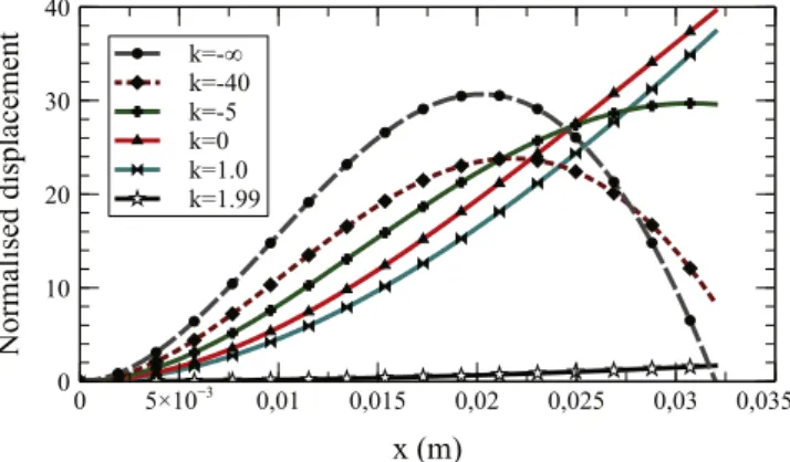
= (figure3) then depicts the effect of this feedback on the modal shapes (see figure 4 for the case of the first mode), and thus on the resonance frequencies for various mass ratios M
μ= .
• k>0 reduces β, that is it decreases resonance frequen-cies, thus it can be assimilated to a softening in the sense that it acts as if the rigidity of the bender were less than in OL. The effect is rather drastic, as for k = 1 thefirst mode will become unstable due to buckling.
• In contrast, k<0 increases β, although rather progres-sively, so a hardening is induced by the CL. Asymptotic analysis shows that for thefirst mode limk→∞β= π.
The theoretical (solid and dashed lines) and measured (crosses and dots) wave numbers are compared for some values of the normalized gain k infigure5. Theoretical values of β are obtained using the secular equation discussed in appendix B. The normalized gains are calculated using the theoretical expression of k, the manufacturer coefficients of table1 and the values of the feedback gains of the amplifier circuit (set to Gc= −{ 40,−26,−20,−13, 0, 13, 20, 26, 40}). Taking into account the gain of the sensor and the flexion rigidity, the reduced gains were k= −{ 1.13,−0.74,
0.57, 0.37, 0, 0.37
− − , 0.57, 0.74, 1.13}. The experimental values of β are deduced from the measured resonance frequencies. Two values of the tip mass to bender mass ratio μ were considered (μ={0.06, 0.54}). The experimental
results are in good agreement with the theoretical prediction.
The effects of the CL on the dissipation are now examined. Due to the variation of β with respect to k, the modal shapesψjare modified, and therefore so are the modal forcesϕj (41). This is depicted infigure6 (top) for the two first modes. Moreover, they affect the modal damping, as can be seen in relations (43) and (44). In this case, assuming that the cross-coupling of the modes is negligible near the mode
Figure 3.Theoretical effect of the normalized feedback gain k on the wave numberβ.
Figure 4.Theoretical effect of the normalized feedback gain k on the modal shapes.
Figure 5.Theoretical (th.) and measured (exp.) wave numberβ versus normalized gain k.
resonance since the considered mode dominates, it is possible to express the CL damping factor as follows:
(
r l s l)
l 1 2 ( ) ( ) ( ) j j q j,11 q j,1 j,1 ξ′ =ξ − ψ + ψ ψ where r l s R l and . q 3 q fl2 2 τ κ = − =The curves of the damping versus k for the caseμ=0.06are presented infigure6, and it can be seen that the feedback has a clear impact, especially on the first mode. Note that to obtain these curves the OL damping was estimated from the OL quality factor on the frequency response. For both modes, the damping vanishes as the gain tends to low values, which indicates a possible instability. The predicted resonance curve of the tip vibration amplitude and phase shift at imposed acceleration are depicted infigure7. The model predictions are in good agreement with the experiment, as for the resonance amplitudes and frequencies. Still, some discrepan-cies can be found, as the experimental resonance curves are non-symmetric, especially for low values of damping. Tests showed that the resonance curves are different for increasing and decreasing frequency sweeping and present amplitude jumps, which is typical of piezoelectrics (soft Duffing resonance). This is out of the scope of the model, and the tests presented in figure 7 are obtained for a decreasing frequency sweep and small acceleration amplitude (0.5 g). Damping is also correctly estimated, in the limit of the model. In figure 8 predictions of the amplitude are compared to experience (top). Furthermore, predictions of the model
taking into account the damping introduced in the CL by the electrical circuit are compared to the prediction including only the mechanical (OL) damping (bottom). This clearly illustrates the combination of both modal forces and damping in the CL. It can be noted that as predicted the system is close to instability, as the feedback gain approaches high positive values and the Bode diagram cannot be plotted due to noisy measurements.
4.2.3. Current at resonance. Finally, figure9 compares the measured and predicted currents delivered by the amplifier to the piezoelectric device at the mechanical resonance frequencies. The theoretical current is obtained by replacing the expression of the derivative of the displacement into (13a) and performing a time derivation:
(
)
i t( ) Q t˙ ( ) 2 SV˙ w˙ L t, . 1 1 1 fl ,1 motional current κ = = −Again, the results are in good agreement. Additionally, the motional current is represented to illustrate the effect of variation of β due to k that results in an inflexion of the motional current curve when the resonant frequency increases.
Figure 6.Theoretical dependence of the modal forces (top) and of the CL damping coefficients (bottom) on the normalized gain k for different values ofμ.
Figure 7.Comparison of the theoretical (plain lines) and measured (dashed lines) dependences of the dynamic mechanical gain (top) and phase (bottom) on the normalized gain k (μ=0.06).
5. Conclusion
This paper proposes an alternative modal decomposition so as to study the effects of feedback on the dynamics of a piezo-electric device. The method is general and consists of the following steps.
• The boundary conditions of the dynamic equation of the system are modified to include directly the feedback as written in (21). Two contributions can be distinguished: reactive (non-dissipative) terms depending on even-time derivatives of the displacement or the spatial derivative
of the displacement, and active terms depending on odd-time derivatives of the same functions.
• A modal analysis, consisting in solving the partial derivative equations when the dissipative terms are cancelled. This results in a set of modal shapes (closed-loop modal shapes) that presents some properties similar to the classical modal decomposition: the equation of motion can still be projected to form an infinite system of independent equations depending solely on time.
• Finally, the dissipative contributions are included as external sources and the solution is then written as a decomposition on the closed-loop modal basis.
The method has been applied to a simple setup that allows us to derive the solutions and has been validated against experimental results. The benefit of the approach is to consider the closed-loop system as a whole system and represent the electromechanical interaction including the control. The classical modal decomposition, obtained by considering the short-circuited resonance, can also be used to obtain this, but the truncation of the projected solution is still the key to the accuracy of the model near a resonance of the closed-loop system. In contrast, the proposed method can efficiently model the dynamics with a few modes. Moreover, some issues such as stability or energy consump-tion can be directly addressed. Therefore, the expected benefits of the method are in the field of design or control of devices where the decoupling of the mechanical structure dynamics and the piezoelectric device is not verified, e.g. energy harvesters such as the one used here, or atomic force microscope tips.
Acknowledgments
This work has been carried out within the framework of the STIMTAC project of IRCICA (Institut de recherche sur les composants logiciels et matériels pour l ’informa-tion et la communica’informa-tion avancée), and the Mint project of Inria. This work is also supported by SEEDS and the FUI Touchit.
Appendix A. Duncan functions Duncan functions are defined as
x x x a
s ( )i =sinh( )+ −( 1) sin( )i (A.1 )
x x x b
c ( )i =cosh( )+ −( 1) cos( )i (A.1 ) with i∈{1, 2}. They fulfil the property
s1,1111=c1,111=s2,11=c2,1=s .1
Figure 8.Measured and predicted mechanical gains at mechanical resonance frequencies (top) and comparison of the model predictions when including the CL damping introduced by the electrical circuit (dashed) or not (plain) (bottom).
Figure 9.Measured and predicted mechanical gains and electrical gains (dots and crosses) and motional current (triangles) at mechanical resonance frequencies.
Appendix B. Expression of the secular equation Defining R R l S S l T T l ( ) , ( ) , ( ) d d d d d d 4 4 4 4 4 4 ⎛ ⎝ ⎜ ⎞ ⎠ ⎟ ⎛ ⎝ ⎜ ⎞ ⎠ ⎟ ⎛ ⎝ ⎜ ⎞ ⎠ ⎟ β β β β β β ′ = ′ = ′ =
the secular equation is obtained after some calculus:
(
)
(
)
(B.1) R l S L T R l S L T ( ) s ( ) ( ) c ( ) ( )s ( ) s ( ) c ( ) ( ) c ( ) ( ) s ( ) ( )c ( ) c ( ) s ( ) 0. d d d d d d 2 2 1 2 2 2 2 2 2 1 1 2 1 2 ⎡ ⎣ ⎢ ⎤ ⎦ ⎥ ⎡⎣ ⎤⎦ ⎡ ⎣ ⎢ ⎤ ⎦ ⎥ ⎡⎣ ⎤⎦ β β β β β β β β β μβ β β β β β β β β β β μβ β − ′ − ′ − ′ × + − − ′ − ′ − ′ × + = ReferencesBallas R G 2007 Piezoelectric Multilayer Beam Bending Actuators: Static and Dynamic Behavior and Aspects of Sensor
Integration Springer Science Business Media
Ducarne J, Thomas O and Deu J-F 2012 Placement and dimension optimization of shunted piezoelectric patches for vibration reduction J. Sound Vib.331 3286–303
Dutoit N E, Wardle B L and Kim S-G 2005 Design considerations for mems-scale piezoelectric mechanical vibration energy harvesters Integr. Ferroelectr.71 121–60
Erturk A 2012 Assumed-modes modeling of piezoelectric energy harvesters: Euler-Bernoulli, Rayleigh, and
Timoshenko models with axial deformations Comput. Struct. 106–7 214–27
Erturk A and Inman D J 2009 An experimentally validated bimorph cantilever model for piezoelectric energy harvesting from base excitations Smart Mater. Struct. 18 025009
Fairbairn M and Moheimani S 2013 A new approach to active q control of an atomic force microscope micro-cantilever operating in tapping mode Proc. 6th IFAC Symp. on Mechatronic Systems (Hangzhou) pp 368–74
Geradin M and Rixen D 2014 Mechanical Vibrations: Theory and Application to Structural Dynamics 3rd edn (Hoboken, NJ: Wiley)
Goldfarb M and Celanovic N 1997 Modeling piezoelectric stack actuators for control of micromanipulation IEEE Trans. on Control Systems17 69–79
Hammond P 1981 Energy Methods in Electromagnetism (Oxford: Oxford University Press)
Ikeda T 1996 Fundamentals of Piezoelectricity (Oxford: Oxford University Press)
Lavrik N V, Sepaniak M J and Datskos P G 2004 Cantilever transducers as a platform for chemical and biological sensors Rev. Sci. Instrum.75 2229
Mason W P 1935 An electromechanical representation of a piezoelectric crystal used as a transducer Bell Syst. Tech. J.14 718–23
Meirovitch L 2002 Fundamentals of Vibration (New York: McGraw-Hill)
Moheimani S O R, Fleming A J and Behrens S 2003 On the feedback structure of wideband piezoelectric shunt damping systems Smart Mater. Struct.12 49
Nadal C, Giraud-Audine C, Giraud F, Amberg M and Lemaire-Semail B 2014 Modelling of beam excited by piezoelectric actuators in view of tactile applications Proc. 11th Int. Conf. on Modelling and Simulation of Electric Machines, Converters and Systems, ELECTRIMACS 2014 (Valencia)
Noliac 2011:www.noliac.com/products/actuators/plate-benders/ show/cmbp05/
Preumont A 2005 On the damping of a piezoelectric truss Mechanics of the 21st Century (Amsterdam: Springer) pp 287–301 Preumont A, de Marneffe B, Deraemaeker A and Bossens F 2008
The damping of a truss structure with a piezoelectric transducer Computers and Structures86 227–39
Smits J G and Choi W-S 1991 The constituent equations of piezoelectric heterogeneous bimorphs IEEE Trans. on Ultrasonics, Ferroelectrics and Frequency Control38 256–70 Tiersten H F 1969 Linear Piezoelectric Plate Vibrations Elements of
the Linear Theory of Piezoelectricity and the Vibrations Piezoelectric Plates (Boston, MA: Springer)
Weaver W, Timoshenko J and Young, D H S P 1990 Vibration Problems in Engineering 5th edn (Hoboken, NJ: Wiley)