Science Arts & Métiers (SAM)
is an open access repository that collects the work of Arts et Métiers Institute of Technology researchers and makes it freely available over the web where possible.
This is an author-deposited version published in: https://sam.ensam.eu Handle ID: .http://hdl.handle.net/10985/18995
To cite this version :
Jianchang ZHU, Mohamed BEN BETTAIEB, Farid ABED-MERAIM - A comparative study of three techniques for the computation of the macroscopic tangent moduli by periodic homogenization -In: 14éme Colloque National en calcul des structures, France, 2019-05-13 - 14éme Colloque National en calcul des structures - 2019
CSMA 2019
14ème Colloque National en Calcul des Structures 13-17 mai 2019, Presqu’île de Giens (Var)
A comparative study of three techniques for the computation of the
macroscopic tangent moduli by periodic homogenization
J.C. Zhu1, M. Ben Bettaieb1, F. Abed-Meraim1
1 Arts et Métiers ParisTech, Université de Lorraine, CNRS, LEM3, F-57000 Metz, France, {jianchang.zhu, mohamed.benbettaieb,
farid.abed-meraim}@ensam.eu
Abstract — The robust and efficient computation of the macroscopic tangent moduli represents a challenging numerical task in the process of the determination of the effective macroscopic properties of heterogeneous media. The aim of the present contribution is to compare the performances of three numerical techniques for the computation of the tangent moduli via the periodic homogenization multiscale scheme: the condensation technique, the fluctuation technique and the perturbation technique. A total Lagrangian approach is adopted in the formulation of the equations governing the periodic homogenization scheme as well as in the derivation of the macroscopic tangent moduli. Through a comparative study, the condensation technique is shown to have better performance as compared to the two other techniques.
Keywords — representative volume element, periodic homogenization, macroscopic tangent moduli.
1. Introduction
In the scientific literature, several multiscale approaches have been proposed to determine the effective properties of heterogeneous media. The analytical approaches developed by Hill [1] and Hashin and Shtrikman [2] are among the earliest proposed multiscale schemes. These approaches have been initially applied to linear elastic composite materials. Despite their wide use in several scientific and engineering applications, the analytical approaches are often limited by the complexity of the studied microstructures and by the presence of geometric and material non-linearities in the modeling. To overcome these limitations, several numerical approaches have been recently developed to estimate the overall mechanical behavior of heterogeneous media. In this field, one can quote the approaches based on the Fast Fourier Transforms [3] and on the Finite Element Method [4]. In the present contribution, attention is focused on the modeling of the mechanical behavior of heterogeneous media exhibiting a periodic distribution of heterogeneities (such as composite materials, hole-containing sheet metals, or polycrystalline aggregates). Considering this spatial periodicity, the periodic homogenization approach is selected to model the transition between the microscopic and the macroscopic levels. The equations governing the periodic homogenization scheme (localization and homogenization relations, equilibrium equations, periodic boundary conditions) are numerically solved by the finite element method. To achieve this task, we have used the toolbox ‘Homtools’ developed by Lejeunes and Bourgeois [5]. Homtools is a set of python scripts for Abaqus that greatly simplify the determination of homogenized characteristics of periodic materials and structures. However, Homtools is unable to determine the macroscopic tangent moduli relating the macroscopic stress measure to the corresponding work-conjugate strain measure. Though, the computation of these tangent moduli is essential in several applications, such as the prediction of macroscopic material or structural instabilities through the bifurcation theory [6,[7], or the modeling of the mechanical behavior of metallic components by the FE2 approach [8]. To remedy this, the present contribution is
devoted to the implementation and comparative analysis of three numerical techniques for the computation of these tangent moduli by periodic homogenization: the condensation technique (CT) developed in [9], the fluctuation technique (FT) presented in [10], and the perturbation technique (PT) detailed in [11]. These numerical implementations have been performed by developing a set of Python
scripts. These scripts are used as post-processing of the finite element computations carried out by
Homtools. This paper is organized as follows:
In Section 2, the periodic homogenization governing equations, within the finite strain framework, are briefly recalled.
The numerical aspects relating to the implementation of the three techniques for the computation of the macroscopic tangent moduli are presented in Section 3.
The performances of these three numerical techniques are assessed in Section 4. Section 5 closes the paper by some conclusions.
2. Periodic homogenization equations
In this paper, a total Lagrangian approach is adopted in the formulation of the governing equations. Accordingly, the deformation gradient and the first Piola–Kirchhoff stress tensor are used as appropriate strain and stress measures, respectively. For the sake of clarity, capital (resp. small) letters and symbols will be used to denote macroscale (resp. microscale) quantities and variables. The periodic homogenization scheme is defined by the following main equations:
The microscopic deformation gradient f is additively decomposed into its macroscopic counterpart F and a fluctuation gradient fper:
,
per
f F f (1)
where fper is a periodic field over the boundary of the representative volume element (RVE) in
its initial configuration.
The averaging relations linking the macroscopic deformation gradient F to its microscopic counterpart f , as well as the macroscopic first Piola–Kirchhoff stress tensor P to its microscopic counterpart p : 0 0 0 0 0 0 1 1 ; V dV V dV V V
F f P p , (2)where V is the initial volume of the RVE. 0
The constitutive relation at the macroscopic scale, relating the rate of the macroscopic first Piola–Kirchhoff stress tensor P to the rate of the macroscopic deformation gradient F through the macroscopic tangent modulus PK1:
= PK1:
P F. (3)
The microscopic static equilibrium equation in the absence of body forces: 0
divx p0. (4)
where x0 is the initial position of the microscopic material point.
The constitutive equations that describe the microscopic mechanical behavior.
3. Computation of the macroscopic tangent moduli
To compute the macroscopic tangent moduli, the RVE is firstly discretized by finite elements as shown in Figure 1. Homtools is used to easily prescribe the periodic boundary conditions on the RVE and to apply the macroscopic deformation gradient F . Once the boundary conditions and macroscopic
deformation gradient are applied, the macroscopic first Piola–Kirchhoff stress tensor P is computed by running the input file generated by Homtools. Further details on these applications can be found in [5]. The macroscopic tangent moduli can then be computed at the convergence of each finite element increment or several increments (this computation frequency has to be specified in the input file of the finite element simulation).
(a) (b)
Figure 1 – Discretization of the RVE: (a) Initial configuration; (b) Deformed configuration.
3.1. Condensation technique
A classical assembly procedure is implemented to determine the global stiffness matrix K from the elementary ones Kel and by taking into account the connectivity of the different nodes of the
mesh: 1 where d K K K B B
e el Nel el el T PK1 e V el V l , (5) with: Nel is the total number of finite elements, B is the elementary gradient matrix,
Ve is the volume of the finite element in the initial configuration,
PK1
l is the microscopic tangent modulus relating p to f .
Then, the lines and the columns of K are rearranged (permuted) to obtain the following decomposition: K K K K K aa ab ba bb , (6)
where b (resp. a ) designates the set of nodes located on the boundary
v
(resp. interior) of the RVE (Figure 1). The macroscopic tangent modulus is deduced on the basis of the following expression:
1 1 1 0 . . . . 1 Q S K K K K S Q PK1 T T bb ba aa ab V , (7)where Q and S are matrix operators, which can be determined by following the procedures detailed in [9].
3.2. Fluctuation technique
The fluctuation method allows us to express the macroscopic tangent modulus PK1 in the
following form [10]: 0 1 1 0 0 0 1 1 ˆ ˆ d K K K
PK1 PK T V V V l V , (8)where K is the global stiffness matrix (defined in Eq. (5)) and ˆK is the global fluctuation matrix
defined as: 1 1 ˆ ˆ with ˆ d K K K B
e el Nel el el T PK e V el V l . (9)3.3. Perturbation technique
The perturbation technique used to evaluate the macroscopic tangent modulus PK1 is based on the
finite difference method. The application of this technique at a given time increment requires to run the finite element computation for ten times (in a 3D case): once to determine the macroscopic tensor
P that satisfies the equilibrium state (called the general step, by following the Abaqus terminology)
corresponding to the loading F , and nine times to numerically build PK1 by slight perturbations of
each component of F (called perturbed steps):
( ) ( ) d ( ) ( ) d F F F ij ij kl ij PK1 ijkl kl kl P P P F F , (10) where ( ) F kl
is the perturbation tensor corresponding to the kl-th component, defined as:
( )
F e e
kl k l
, (11)
and is the magnitude of the perturbation (typically set to 8 10 ).
3.4. Implementation of the three numerical techniques
A set of Python scripts have been developed to implement the different numerical techniques presented in Section 3. To couple the finite element simulations with the Python scripts, some relevant (technical) comments shall be stated:
To apply the condensation technique for elastoplastic media, the microscopic constitutive equations need to be implemented within a user material subroutine (UMAT). Otherwise, using Abaqus built-in constitutive models, the elementary stiffness Kel is determined only on
the basis of the elastic contribution of the microscopic tangent modulus PK1
l (see Eq. (5)). The
elementary stiffness matrices Kel are saved by using the Abaqus command ‘Element Matrix
Output’ in ‘.inp’ file.
To apply the fluctuation technique, a user element subroutine (UEL) needs to be implemented (and not only a UMAT). In this UEL, the elementary stiffness and fluctuation matrices should be determined by Eqs. (5) and (9), respectively. These matrices are saved in external data files. A procedure is also developed in Python scripts to numerically evaluate the integral
0 1 0 d
PK V l V introduced in Eq. (8). As to the perturbation technique, with the toolbox Homtools, the Abaqus/Standard restart technique is used to achieve the perturbed steps. The Python code is devoted to managing the running of the general and the perturbed steps as well as the numerical construction of PK1.
4. Numerical results
4.1. Basic validations
In this section, the implementation of the three techniques (CT, FT, PT) is validated by comparing our numerical predictions with the results published in [12]. To achieve this task, we consider two RVEs of two-phase composites with soft matrix reinforced by stiff inclusions. In the first (resp. second) RVE, the inclusion has the form of a layer (resp. cylinder) as shown in Figure 2 (a) (resp. Figure 2 (b)). The behavior of the different phases is assumed to be isotropic and linear elastic. The Young modulus Em2081.06 MPa and Poisson ratio m0.3007 are assigned to the matrix, and
10
i m
E E , i m to the inclusion.
(a) (b)
Figure 2 – The finite element meshes: (a) Microstructure with layer inclusion; (b) Microstructure with cylindrical inclusion.
The RVEs are submitted to a plane-strain loading. The comparisons between our results and those published in [12] are reported in Table 1. In this table, attention is focused on the analysis of the plane components 1 1111 PK , 1 1122 PK , 1 2211 PK , 1 2222 PK and 1 1212 PK
of PK1 obtained by the different techniques.
Furthermore, to numerically evaluate the difference between our predictions and the results from [12], we have introduced the scalar factor c defined as:
/
PK1 PK1 Ref
c , (12)
where PK1 (resp. PK1 Ref ) defines the Euclidian norm of PK1 determined by our numerical
implementation (resp. published in [12]).
Table 1 reveals that the three techniques provide almost the same results, the scalar factors c=0.996
(microstructure with layer inclusion) and c=0.998 (microstructure with cylindrical inclusion) are very close to the associated values obtained in [12].
Table 1 – Macroscopic tangent moduli for the two RVEs
Ref. [12] CT FT PT
RVE 1 RVE 2 RVE 1 RVE 2 RVE 1 RVE 2 RVE 1 RVE 2
1 1111 PK 78682.6 3413.1 78564.6 3400.7 78564.4 3400.7 78564.5 3400.8 1 2222 PK 4204.0 3413.1 4189.5 3400.8 4189.5 3400.8 4189.5 3400.8 1 1122 PK 1815.9 1415.1 1801.5 1407.2 1801.5 1407.2 1801.5 1407.2 1 1212 PK 1194.0 960.1 1194.0 958.8 1194.0 958.8 1194.0 958.9 c 1.000 1.000 0.998 0.996 0.998 0.996 0.998 0.996
4.2. Comparative performance of the three techniques
The results of Section 4.1 clearly show that all of the three techniques give the same macroscopic tangent moduli. In this subsection, we focus attention on evaluating the performances of these three techniques. To this aim, we consider a cubic RVE made of an elastic cubic inclusion (in the center) and an elastoplastic matrix (Figure 3). The volume fraction of the inclusion is set to 20%.
Figure 3 – The finite element discretization of the RVE with cubic inclusion. The different phases have the following material properties:
Inclusion: the Young modulus and the Poisson ratio are set to 2100 GPa and 0.3, respectively. Matrix: the Young modulus and the Poisson ratio are set to 210 GPa and 0.3, respectively. As to
the hardening behavior, it follows the Swift hardening law:
p
0 184y eq
.
, (13)
where y is the equivalent yield stress and p eq
is the equivalent plastic strain.
The RVE is submitted to an incompressible loading defined by the following macroscopic deformation gradient: 1.2 0 0 0 0.91287 0 0 0 0.91287 F . (14)
The finite element computations generate a set of external files (elementary stiffness matrices for CT, elementary stiffness matrices and fluctuation matrices for FT, and the restart databases for PT), which are used as inputs for the Python scripts. Therefore, the evaluation factor on the computational efficiency is twofold: the required disk space and the CPU time (spent by running the Python scripts). These computations were made on 8 parallelized cores allocated in cluster computer.
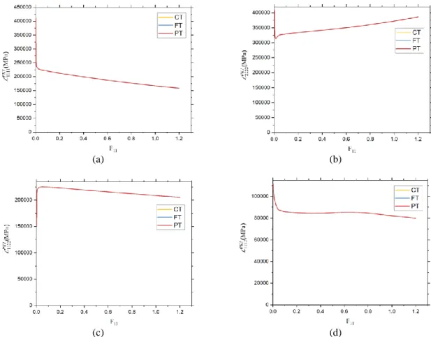
Figure 4 reports the evolution of the components 1111PK1, 2222PK1, 1122PK1, 1212PK1 obtained by CT, FT, PT. This figure reveals that the three techniques give identical results.
(a) (b)
(c) (d)
Figure 4 – Evolution of the plane components of the overall tangent moduli obtained by CT, FT, PT. The macroscopic tangent moduli are evaluated at each 1% of deformation. As shown in Table 2, the CPU times required by CT and FT differ slightly, but the external files generated by FT are much heavier than those generated by CT. PT costs much more CPU times and generates the heaviest external files, but requires very few memory allocation.
Table 2 – Disk space and CPU time required by each of the three techniques for the case of microstructure with cubic inclusion
CT FT PT
External files (GB) 3.979 7.654 11.087 CPU time (Minutes) 82 85.1 111.64
5. Conclusions
Three numerical techniques for the computation of the macroscopic tangent moduli by periodic homogenization have been implemented in the form of Python scripts. All of the three techniques provide the same results. From the computational point of view, the following conclusions can be drawn:
CT appears to be the easiest to be operated and the most efficient in terms of CPU times.
FT does not cost much more CPU times, but it relies on the user subroutine UEL and is more complicated to implement.
PT consumes much more CPU times, and requires the largest disk space.
References
[1] R. Hill, Elastic properties of reinforced solids: Some theoretical principles, Journal of the Mechanics and Physics of Solids, 357–372, 1963.
[2] Z. Hashin, S. Shtrikman, On some variational principles in anisotropic and nonhomogeneous elasticity, Journal of the Mechanics and Physics of Solids, 335–342, 1962.
[3] J.C. Michel, H. Moulinec, P. Suquet, Effective properties of composite materials with periodic microstructure: a computational approach, Computer Methods in Applied Mechanics and Engineering, 109– 143, 1999.
[4] C. Miehe, J. Schotte, M. Lambrecht, Homogenization of inelastic solid materials at finite strains based on incremental minimization principles. Application to the texture analysis of polycrystals, Journal of the Mechanics and Physics of Solids, 2123–2167, 2002.
[5] S. Lejeunes, S. Bourgeois, Une Toolbox Abaqus pour le calcul de propriétés effectives de milieux hétérogènes. 10ème Colloque National en Calcul des Structures, 2123–2167, 2011.
[6] C. Miehe, J. Schroder, M. Becker, Computational homogenization analysis in finite elasticity. Material and structural instabilities on the micro- and macro-scales of periodic composites and their interaction, Computer Methods in Applied Mechanics and Engineering, 4971–5005, 2002.
[7] J.W. Rudnicki, J.R. Rice, Conditions for the localization of deformation in pressure sensitive dilatant materials, Journal of the Mechanics and Physics of Solids, 371–394, 1975.
[8] I. Özdemir, W.A.M. Brekelmans, M.G.D. Geers, FE2 computational homogenization for the thermo-mechanical analysis of heterogeneous solids, Computer Methods in Applied Mechanics and Engineering, 602– 613, 2008.
[9] C. Miehe, Computational micro-to-macro transitions for discretized micro-structures of heterogeneous materials at finite strains based on the minimization of averaged incremental energy, Computer Methods in Applied Mechanics and Engineering, 559–591, 2003.
[10] C. Miehe, J. Schotte, J. Schröder, Computational micro–macro transitions and overall moduli in the analysis of polycrystals at large strains, Computational Materials Science, 372–382, 1999.
[11] C. Miehe, Numerical computation of algorithmic (consistent) tangent moduli in large-strain computational inelasticity, Computer Methods in Applied Mechanics and Engineering, 223–240, 1996.
[12] C. Miehe, J. Schröder, C. Bayreuther, On the homogenization analysis of composite materials based on discretized fluctuations on the micro-structure, Acta Mechanica, 1–16, 2002.