(will be inserted by the editor)
Tubular Structure Segmentation based on Minimal Path
Method and Anisotropic Enhancement
Fethallah Benmansour · Laurent D. Cohen {benmansour, cohen}@ceremade.dauphine.fr http://www.ceremade.dauphine.fr/ ˜{feth, cohen}
the date of receipt and acceptance should be inserted later
Abstract We present a new interactive method for tubular structure extraction. The main application and motivation for this work is vessel tracking in 2D and 3D images. The basic tools are minimal paths solved using the fast marching algorithm. This allows interactive tools for the physician by clicking on a small number of points in order to obtain a minimal path between two points or a set of paths in the case of a tree structure. Our method is based on a variant of the minimal path method that models the vessel as a centerline and surface. This is done by adding one dimension for the local radius around the centerline. The crucial step of our method is the definition of the local metrics to minimize. We have chosen to exploit the tubular structure of the vessels one wants to extract to built an anisotropic metric. The designed metric is well oriented along the direction of the vessel, admits higher velocity on the centerline, and provides a good estimate of the vessel radius. Based on the optimally oriented flux this measure is required to be robust against the disturbance introduced by noise or adjacent structures with intensity similar to the target vessel. We obtain promising results on noisy synthetic and real 2D and 3D images and we present a clinical validation.
1 Introduction
In this paper we deal with the problem of finding a complete segmentation of tubular structures like vessels. The main objective is to extract at the same time the center-line of the tubular structure and its boundary. Such information is useful to diagnose stenoses (on coronary arteries or on carotid for example) using non invasive medical modalities like CT. During the last two decades, the extraction of vascular objects such as the blood vessels, coronary arteries, or other tube-like structures has attracted the attention of more and more researchers. Various methods such as vascular image enhancement methods [53, 30, 16], or others were proposed, see [28, 37] for a complete survey. We will first give a non exhaustive overview of existing variational models for vessels boundary segmentation. Then, some existing methods for boundary and cen-terline extraction are presented.
CEREMADE, UMR CNRS 7534, Universit´e Paris Dauphine, Place du Mar´echal De Lattre De Tassigny, 75775 PARIS CEDEX 16 - FRANCE
1.1 Variational models for vessel boundary segmentation
One of the first variational model for tubular structures segmentation has been in-troduced by Davatzikos and Prince in [10]. They proposed a modified active contour model called ribbon active contour for finding and mapping the outer cortex in 2D brain images, which is a tube-like structure in 2D. Even if this model has been applied only for 2D cortex mapping and suffers from different drawbacks, it was a precursor for different variational model for tube-like structure segmentation.
Siddiqi and Vasilevskiy proposed in [56] a boundary vessel segmentation based on flux maximizing flows. The essential idea is to evolve a curve (in 2D) or a surface (3D) so that it clings to the features of interest in an intensity image. Since then, Descoteaux et al improved in [13] the previous method by choosing a more appropriate vector field that drives the shape evolution. Instead of using the gradient of the image itself, they proposed to use the gradient of Frangi’s [16] vesselness measure. Indeed, this vector field is more appropriate to estimate perpendicular directions of vessels.
Holtzman, Kimmel et al presented in [23] a segmentation method for extracting thin structures in 3D medical images. Their method is based on variational principles. They demonstrated the importance of the edge alignment and homogeneity terms in the segmentation of blood vessels and vascular trees. For that goal, they combined the Chan-Vese minimal variance method [5] with the boundary alignment [27] and the geodesic active surface [3, 4] models.
Gooya et al have made a significant improvement of previous edge detection energy for vessel segmentation in [20, 18, 19]. More precisely, authors of [20] propose to general-ize energy edge detector functional on a Riemannian manifold that describes the local intrinsic orientation of the vessel, using structure tensor. The reason is that the edge detector energy has an isotropic behavior, meaning that it is equally sensitive to image gradients in all directions. Therefore, in a contour propagation scenario, those noisy image gradients parallel to the main orientation prevent further propagation. In fact, sensitivity is mainly needed across the planes normal to the vessel local orientation. The crucial point here is to define a well-behaved Riemannian metric that describes the local orientation of the vessel. Gooya et al utilized in [20] the structural tensor [60] to define their metric. The most significant improvement done by Gooya et al in [20, 18, 19] is the inclusion of vessel orientation in the model by considering a Riemannian edge detector energy.
Here, we recalled some relevant variational methods for vessel segmentation. The main drawback of these method is the time required for fixing parameters and more significantly computation time. Obviously, the listing given here is non exhaustive and it is important to point out recent relevant works along the same research line, like Law and Chung work [34, 33], where they present a vessel segmentation method based on weighted local variance and active contour model. Also, other interesting methods have been presented in [45, 44, 50, 31, 22, 51, 36, 49].
1.2 Vessel boundary and centerline extraction
Deschamps and Cohen [11, 12, 9] proposed to use the minimal path method to segment tubular structures. The minimal path technique introduced by Cohen and Kimmel [8] captures the global minimum curve1between two points given by the user. This leads to
the global minimum of an active contour energy. Unfortunately, despite their numerous advantages, classical minimal path techniques exhibit some disadvantages. First, vessel boundary extraction can be very difficult, even in 2D where the vessel’s boundary can be completely described by two curves. Second, the path given by the minimal path technique does not always yield to the centerline of the vessel. A readjustment step is required to obtain a central trajectory. Third, the minimal path technique provides only a trajectory and does not give information about the vessel boundary and local width.
In [11, 12] Deschamps and Cohen, demonstrated that the front propagation could be stopped on the basis of a distance traveled by the front corresponding to the known length of the minimal path to the starting point while the front is propagated. When the propagation speed is almost constant inside the tubular shape, this length is almost the geodesic distance to the starting point inside the tubular object. However, classical segmentation problems do not provide an excellent contrast like air-filled colon on CT scanner, and the front usually flows over the boundaries of longer and thinner objects when propagating. Therefore, Cohen and Deschamps showed in [9] how the Fast Marching surface segmentation can be specifically optimized for this target. Indeed, it appears inefficient to use all points of the propagating front in the computation of the arrival time in the Eikonal equation. The idea presented in [12, 9] is that some of them located in the tail of the propagating front could be considered as walls, thus blocking the leakage that occurs. This Freezing process can be done by setting their speed to zero. Freezing points during propagation means we consider the front has reached the object boundaries when it visits them. Two Freezing criterion have been proposed in cited papers. The first one is time-based and the second one is distance-based. Once the contour of a vessel is obtained, authors of [11] proposed a method to extract a centerline inside it.
Li and Yezzi proposed in [38, 39] a new variant of the classical, purely spatial, minimal path technique by incorporating an extra non-spatial dimension into the search space. Each point of the 4D path (after adding the extra dimension for the 3D image) consists of three spatial coordinates plus a fourth coordinate which describes the vessel thickness at that corresponding 3D point, see figure 1 as a 2D example. Thus, each 4D point represents a sphere in 3D space, and the vessel is obtained by taking the envelope of these spheres as we move along the 3D curve. A crucial step of this method is to build an adequate potential that drives the propagation. Li and Yezzi [38, 39] proposed different isotropic potentials. Since potentials proposed by Li and Yezzi are very parameter dependent, an important perspective of their work was the construction of a more appropriate potential. Moreover, by considering only isotropic metrics, Li and Yezzi did not take into account the vessel orientation.
Along the same research line, Mohan et al [48] used the 4D minimal path model of Li and Yezzi [38, 39] for segmenting the Cingulum Bundle from DW-MRI. After adding the extra non spatial dimension (the radius dimension), they associated to the path an anisotropic potential related to the Finsler metric. Let us denote ˜γ(u) = (γ(u), r(u)) the 4D path with arc length parameterization (i.e k˜γ0k2 = 1) and S2 ⊂ R3 the 2D
sphere. The considered energy is:
E(˜γ) = Z ˜ γ P „ ˜ γ(s), γ 0(s) kγ0(s)k « ds, (1)
Fig. 1 A tubular shape is presented as the envelope of a family of spheres or disks with continuously changing center points and radii.
where this time1, the potential is P : R4× S2→ R∗
+. Authors of [48] gave two different
choices of P that are meaningful for extracting the Cingulum Bundle from DW-MRI, both based on local region statistics. In order to optimize energy functional (1), they used gradient descent method where the gradient direction is computed with respect to a geometrized Sobolev metric [57] instead of the classical L2 metric which is very unstable according to [46]. An important contribution of Mohan et al [48] is that they considered orientation of the vessel in their energy model, which is reasonable for tubu-lar structures. But the proposed potentials were defined in an ad hoc manner. Moreover, in the energy functional given by equation (1) the derivative of the non spatial dimen-sion r0(s) is not taken into account. That makes their model very insensitive to the radius dimension and inappropriate for tubular structures with varying radii, which is not the case of Cingulum Bundle.
1.3 Contributions
In this paper we propose a vessel segmentation method based on a minimal path formulation and anisotropic enhancement. Both vessel orientation and width are taken into account. Our contribution is threefold:
• First, inspired from [38, 39], we introduce a minimal path model, that takes into account the vessel width, by adding an extra dimension, and the vessel orientation by considering anisotropic metrics.
• Next, we propose a well motivated metric constructor for the anisotropic metric based on the Optimally Oriented Flux (OOF), introduced by Law and Chung in [32], by using its scalar function as well as its orientation (while authors of [32] used only the scalars, that is the eigenvalues). That makes the propagation faster along the vessels centerline and for exact associated scale. This means that the path location, orientation and scale (radius) have to be coherent with the local geometry of the image extracted by the OOF.
• Finally, we make a deep analysis of the chosen enhancer by establishing a link between the OOF and the widely used Hessian-based tubular structure enhancers like Frangi’s [16], and by demonstrating an interpretation of the OOF in terms of steerable filters [17, 25].
1 In the classical Finsler formulation, the potential is under the form P : Rn× Sn−1→ R∗ +.
1.4 Paper outline
In section 2, we give some background on the minimal path method and Anisotropic Fast Marching. In section 3 the Optimally Oriented Flux descriptor is presented, a link between the OOF and the Hessian-based vesselness measures is established, Oriented Flux filter is interpreted in terms of steerable filters, and the metric design is shown. In section 4, first, we show advantages of anisotropy. Second, results on synthetic and real data are shown. Third, validation results are given. Finally, conclusions and perspectives follow in section 5.
2 Background on the Minimal Path Method 2.1 Formalism
A geodesic is a path, linking two points, that globally minimizes an energy functional weighted by an image potential. Hence, a geodesic is also called minimal path. Without loss of generality and in order to simplify notations we will assume hereinafter that a path γ is parametrized along its length (i.e kγ0k = 1). The energy minimized by a geodesic is under the form:
E(γ) = Z
γ
P`γ(s), γ0(s)´ds. (2)
Such formulation has been first presented to the computer vision community by Cohen and Kimmel [8] in the particular isotropic case, when P > 0 does not depend on the orientation of the path.
This energy corresponds to the length of a curve in a Finsler2 manifold [46]. In this paper, we are interested only on the particular case of Riemannian manifold, that is the potential is under the form P(γ(.), γ0(.)) =pγ0(.)TM(γ(.))γ0(.) describing an
infinitesimal distance along a pathway γ relative to a metric tensor M (symmetric definite positive). Thus, we are considering only the case of an elliptic3 medium. In the isotropic case M(.) = P2(.)I, where I is the identity matrix. A curve connecting a point p1to p2that globally minimizes the above energy (2) is a minimal path between
p1and p2, noted Cp1,p2 and also called a geodesic.
The solution of this minimization problem is obtained through the computation of the minimal action map U : Ω → R+associated to p1on the domain Ω ⊂ Rd (in this
paper d = 2, 3 or 4). The minimal action is the minimal energy integrated along a path between p1 and any point x of the domain Ω :
∀ x ∈ Ω, U (x) = min γ∈Ap1,x ( Z γ P`γ(s), γ0(s)´ds ) , (3)
where Ap1,xis the set of paths linking x to p1. The values of U may be regarded as the
arrival times of a front propagating from the source p1with oriented velocity related
to the metric tensor M−1. U satisfies the Eikonal equation
k∇U (x)kM−1(x)= 1 for x ∈ Ω, and U (p1) = 0, (4)
2 Finsler geometry is just Riemannian geometry without the quadratic restriction [6]. 3 A Riemannian metric is described by a symmetric definite positive tensor field: M. Each
where kvkM =
√
vTM v. The map U has only one local minimum, the source point
p1, and its flow lines satisfy the Euler-Lagrange equation of functional (2). Thus, the
minimal path Cp1,p2 can be retrieved with a simple gradient descent on U from p2
to p1 (see Fig. 2), solving the following ordinary differential equation with standard
numerical methods like Heun’s or Runge-Kutta’s : dCp1,p2
ds (s) ∝ −M
−1
(Cp1,p2(s))∇U`Cp1,p2(s)´, with Cp1,p2(0) = p2. (5)
Equations (4) and (5) have been presented under their isotropic version in [8]. The Eikonal equation (4) belongs to the class of static Hamilton-Jacobi equations. The associated unique viscosity solution [42] U satisfies the Hopf-Lax formula which is given by equation (3) in our case4, see for example [2, 24, 1] for more details. The proof of equations (4) and (5), in the general case, can be found in [42]. This general proof requires notions from calculus of variations [15].
Fig. 2 Minimal path examples on an isotropic case on the left image. On the middle, visual-ization by small ellipses of eigenvalues of a metric constant on each half side of the image. On the right, the minimal action map associated to the source point p1 with the minimal path
Cp1,p2.
On figure 2, we show some examples of the minimal path method on an isotropic case and an anisotropic one. On the first image of figure 2 the metric is isotropic and the potential P in the grey region is half of the white one. Isolevel sets of the minimal action map associated to the source point p1 are displayed together with a minimal
path Cp1,p2. The second image represents a metric M (M
−1 is displayed). We took
two constant metrics in each half side of the image with different orientations. On the last image, the minimal action map U associated to the metric M and to the source point p1is shown. The minimal path Cp1,p2 is found by solving equation (5). We can
see that the minimal path tries to agree as much as possible with the orientation of the ellipses.
2.2 Eikonal solvers 2.2.1 Short overview
In this section we are interested in solving numerically the Eikonal equation (4). In the last two decades, considerable efforts have been made to develop numerical methods for solving static Hamilton-Jacobi equation (which includes the Eikonal equation) on
4 Indeed, it is easy to show that, in our case, the required conditions for existence and
regular or unstructured meshes. The reader is referred to the literature for rigorous and more precise statements.
One of the first consistent discretization on a regular grid of equation (4), in its isotropic version, has been proposed by Rouy and Tourin in [52]. They proposed an upwind finite difference discretization of the Eikonal equation k∇U k = P on a regular grid. They showed that the associated discrete solution converges toward the viscosity solution5; and an iterative algorithm based on a nonlinear variant of the Gauss-Seidel iteration has been proposed to compute the discrete values. A few years later, Sethian [54] proposed a single-pass algorithm to compute the solution of the upwind discretiza-tion. The algorithm proposed by Sethian, called Fast Marching is based on Dijkstra’s algorithm for computing shortest paths on graphs [14]. Independently, Tsitsiklis [58] proposed a similiar Dijkstra-like algorithm to solve numerically the isotropic Eikonal equation. However, the used discretization is not based on the Eikonal equation itself but on the Hopf-Lax formula (given in a particular case by equation (3)).
Both Sethian’s and Tsitsiklis’s methods [54, 58] are suitable for isotropic metrics, but they fail for anisotropic metrics according to [7]. To deal with anisotropy, three different improvements of the classical fast marching method have been proposed:
1. change the local approximation scheme as done by Lenglet et al in [35],
2. introduce a recursive approach as done by Konukoglu et al in [29], they called the proposed method Recursive Fast Marching,
3. extend the neighborhoods, depending on the local anisotropy as done by Sethian and Vladimirsky in [55], or in a fixed manner as done by Lin in [40] and used by Jbabdi et al in [26].
Convergence toward the viscosity solution of the anisotropic Eikonal equation (4) has been proved only for the Ordered Upwind Method (OUM), using an extended neigh-borhood, in [55]. The main drawback of the OUM is that, for high anisotropy, the neighborhood needed for the local update is extremely vast.
Other iterative approaches to solve the anisotropic Eikonal equation have been proposed. In [2], Bornemann and Rasch presented a linear finite-element discretiza-tion for static Hamilton-Jacobi equadiscretiza-tions on unstructured trianguladiscretiza-tions. Similarly to Tsitsiklis [58], their discretization is based on the Hopf-Lax formula. Bornemann and Rasch proposed to use a tricky adaptive Gauss-Seidel iteration to solve the underlying system of non-linear equations. Convergence results have been shown in [2] under some assumptions that are easy to satisfy in our Riemannian case.
In this paper we used Lin’s scheme to approximate the solution of the anisotropic Eikonal equation, since it is much faster (than OUM and the iterative algorithm pro-posed in [2]) and, as long as the anisotropy remains reasonable, the introduced errors do not affect much the extracted geodesics.
2.2.2 Fast Marching Algorithm
The FMM is a front propagation approach that computes the values of U in increasing order, and the structure of the algorithm is almost identical to Dijkstra’s algorithm for computing shortest paths on graphs [14]. The main difference is the expression of the local contribution to the weighted distance. In the course of the algorithm, each grid point is tagged as either Alive (point for which U has been computed and frozen),
Trial (point for which U has been estimated but not frozen) or Far (point for which U is unknown). The set of Trial points forms an interface between the set of grid points for which U has been frozen (the Alive points) and the set of other grid points (the Far points). This interface may be regarded as a front expanding from the source until every grid point has been reached. Let us denote by Nm(x) the set of m neighbors of
a grid point x, where m = 3d− 1 if the dimension of Ω is equal to d. Initially, all grid points are tagged as Far, except the source point p1 that is tagged as Trial. At each
iteration of the FMM one chooses the Trial point with the smallest U value, denoted by xmin. Then, xminis tagged as Alive and the value of U is updated for each point of
the set Nm(xmin) which is either Trial or Far. In order to satisfy a causality condition,
the way U is updated in the vicinity of xmin requires special care. The iteration ends
by tagging every Far point of the set Nm(xmin) as Trial. The algorithm automatically
stops when all grid points are Alive. The key to the speed of the FMM is the use of a priority queue to quickly find the Trial point with the smallest U value. If Trial points are ordered in a min-heap data structure, the computational complexity of the FMM is O(N logN ), where N is the total number of grid points.
A crucial step of the Fast Marching algorithm is the computation of the weighted distance between the front and the neighboring voxels in the Trial set. Here, we present a way to estimate this weighted distance in the anisotropic case and only in 3D. It is straightforward to extend it to 4D. Since the distance is anisotropic, we cannot use the standard methods, because they rely on the fact that the geodesics are perpendicular to the level sets of U . To take into account the anisotropy (recall that the proposed solution here does not converge toward the viscosity solution of equation (4)), and without using a vast neighborhood, Lin [40] and Jbabdi et al [26] considered a set of simplexes that cover the whole neighborhood around a voxel of the front. The definition of a simplex neighboring a point x is simply a set of three points (x1, x2, x3) that are
among the 26 neighbors of x, such that x1 is a 6-connectivity neighbor, x2 is a
18-connectivy (and not 6-connectivity) neighbor, and x3 is a 26-connectivity (and not
18-connectivity) neighbor. This set of points defines a triangle that we denote x1x2x3.
There are 48 such triangles around x for the 26 connexity, see figure 3.
Fig. 3 On the left Position of the optimal point on a simplex such as to minimize the geodesic distance to x. On the right the considered simplexes.
If the geodesic passing by xmcomes from a triangle x1x2x3then the time of arrival
is given by: U (xm) = min x∈x1x2x3 n U (x) + Z xm x P (γ, γ0)o (6)
where point x can be interpreted as a virtual source6 on the triangle. To estimate U (xm), where xmis a neighbor of the last trial point xmin, we make two approximations
on the term one wants to minimize. First, we assume the path between x and xmto
be a segment and the metric to be constant along this segment, equal to its value at point xm. Hence, we want to minimize:
F (x) = U (x) + kx − xmkM(xm), (7)
Then, since the point x is in the triangle x1x2x3, we can replace x by its barycentric
expression x =P3
i=1αixi, where α = (α1, α2, α3) withPiαi = 1 and αi ≥ 0; and
make a linear approximation of its U -value. We then have to minimize:
f (α) = 3 X i=1 αiU (xi) + ‚ ‚ ‚ ‚ ‚ xm− 3 X i=1 αixi ‚ ‚ ‚ ‚ ‚ M(xm) . (8)
This equation follows Tsitsiklis’s approximation [58]. The function f is convex and the constraints on α, i.eP3
i=1αi = 1 and αi ≥ 0, define a convex subset. Thus the
minimization of f can be done using classical optimization tools. See appendix B of [26] for more details.
Solving this minimization for each triangle, we get a value Ux1x2x3. Finally, we
choose the triangle giving the smallest value. Note that in order to approximate ∇U , computing the derivatives of U in the triangle using the estimate U (xm) gives a
con-sistent approximation of ∇U (xm) by the following:
∇U (xm) = (U (xm) − U (x?)) xm− x ?
kxm− x?k, (9)
where x?is the minimizer of function f (see figure 3 left) and k.k is the Euclidean norm. The computation of the gradient is very useful since it is used to solve the gradient descent described by equation (5).
2.3 Comparison and Discussion
In this section, we are going to compare numerical results and computation time of Lin’s algorithm and the iterative algorithm of Bornemann and Rasch on a relevant example. For this purpose, we designed an anisotropic metric from the left image of figure 4.
The designed metric has high anisotropy along the spiral and is isotropic almost every where else with low propagation velocity. Such metric is constructed using meth-ods presented later (section 3.4), namely equation (20) at the associated fixed scale (r = 3 pixels) of the spiral. Indeed we took a maximal anisotropy ratio equal to 100. Geometrically the maximal anisotropy ratio corresponds to the maximal ratio between the major and minor axis of ellipsoids displaying the metric (see figure 2 middle for example). On the second image of figure 4, the computed minimal action map U , using the Fast Marching algorithm presented in section 2.2.2, from the source point p1and
the minimal path Cp2,p1 are displayed.
6 This formulation is based on Huygens-Fresnel principle from geometric optics and problems
Fig. 4 From image on the left, an anisotropic metric with high anisotropy ratio (µ = 100) along the spiral is constructed. Second image, geodesic distance from source point p1computed
using Lin’s algorithm and a geodesic Cp1,p2. On third image, the geodesic distance is computed using Bornemann & Rasch algorithm. The last image displays the number of iterations for Bornemann & Rasch algorithm at each point in the image domain, until the convergence criterion is satisfied.
One can see that a shortcut occurs. Actually this is due not to the metric but to the introduced errors by the chosen Eikonal solver (Lin’s Fast Marching algorithm). Indeed, we implemented Bornemann and Rasch algorithm [2] to solve the same problem, and obtained the result shown in the third image of figure 4. It has been shown in [2], and numerically verified by our care, that the proposed iterative algorithm converges to the viscosity solution. However, the main drawback of Bornemann and Rasch algorithm is the computation time. On the right image of figure 4, one can see the number of iterations needed in order to mend the minimal action map values. Some points need to be updated up to 500 times. The computation time of the iterative algorithm for this spiral image of size 548 × 600 is about 2 minutes, while the computation time of the Fast Marching algorithm is less than a second. For higher dimensions, one can imagine that the computation time of the iterative algorithm [2] is heavily long.
As a matter of fact, there is a tradeoff between efficiency and accuracy. On the one hand, using the Fast Marching algorithm provides reasonable results as long as the anisotropy ratio remains small; disabling us for taking complete advantage of the Tubular Anisotropy method presented in this paper. On the other hand, one can in-crease the anisotropy ratio and use Bornemann and Rasch iterative algorithm but this choice considerably penalizes the efficiency7 of the whole algorithm.
Unlike the Fast Marching algorithm, the iterative algorithm is parallelizable. In [59], authors propose an efficient implementation on parallel architectures to compute geodesic distances on geometry images. An important perspective is to make a similar parallelized implementation of Bornemann and Rasch’ algorithm in order to genuinely take advantage of the Tubular Anisotropy method.
3 Optimally Oriented Flux : an Anisotropy Descriptor
We are interested in the construction of a metric that extracts from the image the geometric information leading to reconstruction of vessels. This means that we wish to find an estimate for the local orientation and scale and a criterion on the local geometry to distinguish the presence of vessels from the background. First, we tried some existing
7 The complexity of the algorithm proposed in [2] is O(C
µN1+1/d), where d is the dimension
of the image and N the total number of grid points, compared to O(N log(N )) for Lin’s [40]. It has been shown empirically (by our care) that Cµis an increasing function on µ. Actually,
vessel enhancers like the Hessian-based vesselness measures [16, 53, 43, 41]. The main drawback of these enhancers is that they include adjacent features. The anisotropy descriptor presented here is inspired from the optimally oriented flux (OOF) recently introduced by Law and Chung in [32]. Its main advantage is that adjacent objects are not taken into account. Moreover, this descriptor provides intuitively a good estimate of vessel direction enabling us to design a suited anisotropic metric for the oriented minimal path model presented in the previous section. Also, we establish a link between the OOF and the Hessian-based enhancers that justifies our choice.
3.1 Definitions
At the position x on an image I, the oriented flux is the amount of the image gradient projected along the axis v flowing out from a 3D local sphere8(or a 2D circle) Sr. It
is measured as in [32], f (x, v; r) =
Z
∂Sr
((∇(G ∗ I)(x + h) · v)v) · nda, (10) where G is a Gaussian function with a scale factor of 1 pixel, r is the radius of the sphere (or circle), h = rn is the relative position vector along ∂Sr, with n the outward
unit normal of ∂Sr, and da is the infinitesimal area (or length) on ∂Sr. Function f is
the flux of the smoothed image gradient ∇(G ∗ I) projected along direction v toward the sphere ∂Sr. To detect vessels having higher intensity than the background region,
one would be interested in finding the vessel direction which minimizes f (x, v; r), i.e. we are looking for:
arg min
v f (x, v; r). (11)
Using the divergence theorem, it can be shown that f (x, v; r) is a quadratic form on v and its associated matrix can be calculated using a simple convolution,
f (x, v; r) = vT ˘I ∗ (∂i,jG) ∗1Sr(x)
¯
v := vT {I ∗ Fr(x)} v, (12)
where (∂i,jG) is the Hessian matrix of function G and 1Sr is the indicator function
inside the sphere (or circle) Sr. Fr is called the oriented flux filter. By differentiating
the above equation with respect to v, minimization of function f is in turn acquired as solving a generalized eigenvalue decomposition problem. Solving the aforementioned generalized eigen decomposition problem gives d eigenvalues (where d = 2 or 3 is the dimension of the image), λ1(·) ≤ · · · ≤ λd(·) and d eigenvectors vi(·), i.e. λi(x; r) =
f (x, vi(x; r); r) for i = 1, . . . , d. To handle the vessels having various radii, a
multi-scale approach should be used along with the OOF method. In [32], Law and Chung have proposed to normalize the OOF’s eigenvalues by the sphere surface area when the OOF method is incorporated in a multi-scale approach for 3D image volumes. In the 2D case the eigenvalues are normalized by the circle perimeter 2πr. In the 3D case the eigenvalues are normalized by the sphere area 4πr2.
In the 2D case (see figure 5), for a point on the centerline and if r is equal to the radius of the vessel, the first eigenvector v1represents the direction orthogonal to the
vessel. v2 is the estimated direction of the vessel. If the point is inside the vessel but
not on the centerline (for example, point x2in figure 5-(a)), the OOF response provides
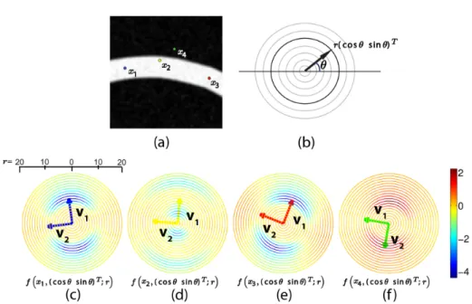
Fig. 5 The plots of the values of f (x, v; r) obtained from the synthetic image shown in the top, at four different positions with various radii and projection axes. (a) Four interesting positions, denoted as x1, x2, x3 and x4 are shown along with the original synthetic image.
(b) An illustration regarding the polar coordinate system used in (c)-(f). (c)-(f) The plots of the values of f (·) and the corresponding eigenvectors, computed at the four different positions shown in (a), using various values of r and different projection axes (cos θ sin θ)T.
two local minima, when v is parallel to the vessel centerline and for the two possible scales, see figure 5-(d). Finally, if the point is outside the vessel and near its boundary, the estimated vessel direction, i.e v2, which is the eigenvector associated to the largest
eigenvalue is perpendicular to the vessel direction.
In the 3D case, if the point is on the centerline, the two eigenvectors associated to the first eigenvalues (λ1, λ2) represent the directions orthogonal to the vessel direction.
v3goes along the vessel, see figure 6. On the same figure, one can see that if the point
x is on the centerline, the minimal response of the function f is obtained when the radius r is equal to the exact radius of the tube. If the point is inside the tube but not on the centerline, v3is parallel to the tube orientation, and the other eigenvectors
depends on the scale r. If the point is outside the tube (last line), then the vector v3,
corresponding to the red area, is oriented toward the centerline.
3.2 OOF as a steerable filter
In this section, we will demonstrate that the Optimally Oriented Flux function f can be interpreted in terms of steerable filters [17]. Steerable filters are useful to detect edges or ridges (vessel-like structures) at any orientation. Steerable filters are filters for which the response at different orientations can be synthesized from linear combination of rotated versions of itself (this is called steerability relation). More precisly a filter
Fig. 6 Plot of f (x, v; r) superimposed on the original 3D synthetic image for three different points (on each line) and different values of the radius : r = 4, . . . , 7 from left to right. The radius of the tube on the top half side image is equal to 4, and equal to 6 on the bottom half side. Similarly to figure 5, the visualization of the normalized flux function is done using a spherical coordinate system (instead of the polar one used in 2D). The first point is on the centerline of the tube. The second point is inside the tube but not on the centerline. The third point is outside the tube. The reader should zoom on each image. Notice that the colormaps are different for each point.
F : R2→ R is said to be steerable if F (Rθx) = M X i=1 ki(θ)F (Rθix) (13)
where Rθis the rotation matrix:
Rθ=
„ cos(θ) sin(θ) − sin(θ) cos(θ) «
and x = (x, y) is a point in R2. Inspired by the steerability property of the Hessian filter presented in [25], we will show that the oriented flux filter is steerable as well. We will compare the associated template features of the Hessian and the oriented flux in order to justify qualitatively our choice.
Jacob and Unser [25] showed that the popular ridge filter based on the Hessian matrix [16, 53, 43, 41] can be interpreted as a steerable filter and that this filter can be synthesized by a template which is ∂xxgr(the second derivative along x direction of a
Gaussian grat scale r). The steerability relation can be expressed in a matrix form as follows: ∂xxgr(Rθx) = uTθ „∂xxgr(x) ∂xygr(x) ∂yxgr(x) ∂yygr(x) « uθ (14)
= cos2(θ)∂xxgr(x) + sin(2θ)∂xygr(x) + sin2(θ)∂yygr(x),
where uθ= (cos(θ), sin(θ))T. Hence three representative directions of the Hessian filter
are (θ1= 0, θ1= π4, θ2=π2) associated to the fonction basis: (∂xxgr, ∂xygr, ∂yygr) (see
equation (13)).
It has been shown by Law and Chung [32], and rewritten by equation (12) that the response given by the optimally oriented flux can be expressed as a convolution of the image I with vTFrv, called here oriented flux filter. At a given orientation v = uθthe
oriented flux filter can be synthesized as follows:
uTθFr(x)uθ= {∂xxG ∗1r} (Rθx). (15)
We conclude that the oriented flux filter is a steerable filter and that an associated template is ∂xxG ∗1r. This result is straightforwardly extensible to higher dimensions.
Fig. 7 Feature templates associated to the Hessian (on the left) and to the oriented flux (on the right) at the same scale r. The yellow dotted line simulates the vessel direction. σ is the variance of G.
In figure 7, the templates associated to both the Hessian filter and the oriented flux filter are shown. Hence, we can qualitatively justify that the OOF is more suited for vessel enhancement and orientation detection. Indeed, unlike the Hessian template, the oriented flux template profile is more localized around the vessel boundaries. Thus, adjacent features to the vessel, like heart chambers or other organs, will most likely not be included by the OOF. In the next section we will highlight a link between the OOF and the Hessian-based filters in order to justify again the choice of the OOF for our medical application.
3.3 Unifying Flux Based and Hessian Based vessel enhancement
Let us recall the optimally oriented flux, and the Hessian formulations. It has been shown that the flux of the image gradient projected along a direction v through a sphere of radius r can be written as follows,
f (x, v; r) = Z ∂Sr ((∇(G ∗ I)(x + h) · v)v) · h |h|da = v T Q(x; r)v where Q(x; r) = “ `∂i,jG ´ i,j∗1Sr∗ I ” (x) (16)
where (∂i,jG) is the Hessian matrix of function G and 1Sr is the indicator function
inside the sphere (or circle) Sr, and G is a Gaussian with a scale σ equal to the size
of a voxel (or a pixel). The vesselness measure proposed by Law and Chung in [32] is based on the eigenvalues of Q.
The Hessian-based vesselness measures proposed in [16, 53, 43, 41] are based on the eigenvalues of the scaled Hessian of the image:
H(x; r) = ((∂i,jGr)i,j∗ I)(x),
where (∂i,jGr)i,j is the Hessian of the Gaussian function Grwith scale r. Finding the
eigenvalues of H is similar to find optimal directions of the associated quadratic form. For a vector v, the quadratic form associated to the Hessian matrix is:
h(x, v; r) = vTH(x; r)v = vT˘((∂i,jGr)i,j∗ I)(x)¯ v
= vT Z Rd ∂i,jGr(h)I(x + h)dh ff i,j v. Using integration by parts one can show that:
Z Rd ∂i,jGr(h)I(x + h)dh = − Z Rd ∂Gr ∂xj (h)∂I ∂xi (x + h)dh, hence, h(x, v; r) = vTH(x; r)v = − Z Rd ((∇I(x + h).v)v).∇Gr(h)dh.
Recall that the Gaussian function is spherically symmetric. Thus, one can write Gr(h) =
gr(khk) = gr(R) = (r√12π)dexp(−
R2
2r2), yielding to ∇Gr(h) = g0r(khk)n, where n is
the outward normal to the sphere of radius R. Therefore, using reduction formulae, one can show that:
h(x, v; r) = − Z+∞ 0 gr0(R) „Z ∂SR ((∇I(x + Rn).v)v) .nda « | {z } (I) dR, (17)
where da in term (I) is the infinitesimal area (or length) on the surface sphere ∂SR.
One can recognize the term (I) of equation (17) as the oriented flux introduced by Law and Chung in [32] (without the smoothing term). As a matter of fact, one can interpret function h as a pondered flux of the projected image gradient along direction v toward spheres. In figure 8 the normalized weight function associated to the Hessian is presented. One can see that contrary to the Hessian, the OOF weight function (which is
the indicator function for Sr) takes into account only the values of the image gradient
on the circle of the desired scale. That explains the behavior of the Hessian based vesselness measure, as shown in figure 4 of [32], which misses vessels of weak intensity especially when they are adjacent to other structures (arrows 5 and 6). Indeed, if one considers that the influence of adjacent objects is significant until some threshold T of the weight function (for example the red line in figure 8 corresponds to T = 0.5), then all objects in the vicinity of the desired point with distance to the desired point in [βr, αr] are taken into consideration. This is the weak point of the Hessian based vesselness measures, that is, adjacent structures are taken into consideration, and hence distort the measure. As an example, for T = 0.5, we have α ≈ 0.32 and β ≈ 1.9. One can conclude that the Hessian based vesselness measure is not an appropriate choice when the desired vessels are adjacent to other features in the image, which usually happens in nature.
Fig. 8 Profile of the normalized flux weighting function g 0 r(R) g0 r(r) = Rgr(R) rgr(r) associated to the Hessian.
We showed here, that the Hessian based vesselness measures may include adjacent structures yielding to bad results. The point is that the flux weighting function (see figure 8) associated to the Hessian matrix is too much extended around the desired scale, i.e. when R/r = 1. Meanwhile, the weighting function associated to the Optimally oriented flux is the indicator of R = r, hence it assumes that vessels response on the image is perfectly contrasted and with uniform intensity. On natural images, this assumption is obviously not satisfied.
In order to improve the vesselness measure response, one has to choose a flux weighting function that is in between the very discontinuous indicator function and the very extended profile given by the derivative of the Gaussian (see figure 8). Obviously, flux weighting function has to depend on the response of tubular structures on the image which depends on many parameters like image modality, type of vessels (coronary, pulmonary or other arteries), the used contrast agents...etc. An important question to raise here is the following: Is there an optimal way to define a weighting function for some desired arteries on a given image ? And therefore, what are these meaningful
optimality conditions one can impose on the weighting function ? These questions remain open. One perspective of this work is to define a set of meaningful optimality conditions and to find the optimal weighting function associated to them as a learning step.
3.4 How to design the metric
Our main contribution is to impove Li and Yezzi method [38, 39] (see section 1.2 above) by adding to it an anisotropic formulation, and the anisotropic metric is constructed by extension of the OOF descriptor presented by Law and Chung [32].
We consider (d + 1)D minimal path that minimizes the following energy: Z
γ
nq
γ0(s)TM(γ(s))γ0(s)ods, (18)
where M is the (d + 1)D anisotropic metric we want to construct. It is not natural to consider orientations on the (d + 1)thdimension, i.e the radius dimension. Thus we propose to decompose by blocks the matrix M as follows:
M(x, r) = „ ˜ M(x, r) 0 0 Pradius(x, r) « (19)
where ˜M(x, r) is a d×d symmetric definite positive matrix giving the spatial anisotropy and Pradius(x, r) is the radius potential (also strictly positive).
Since the result given by the anisotropic minimal path method is very dependent on the metric, results inherit advantages and drawbacks of the constructed metric, and we should be very careful with its construction. First, let us fix conditions on the desired metric. The spatial metric M has to be well oriented along the vessel˜ centerline. And the radius potential Pradiushas to be small for the adequate scale for
any point of the image.√Pradius corresponds to the inverse velocity along the radius
dimension. SinceM is symmetric definite positive, one can decompose it as follows:˜ ˜
M(.) =Pd
i=1mi(.)ui(.)ui(.)T, where 0 < m1≤ · · · ≤ mdare the eigenvalues and ui
are the associated eigenvectors. The velocity of the propagating front along direction ui is equal to 1/
√
mi. In order to design the metric, let us recall that the oriented
flux matrix is symmetric (but not necessarily positive), and it can be decomposed as follows: Q(.) =Pd
i=1λi(.)vi(.)vi(.)T. The metric M has to be definite positive, and
we want to make the propagation faster along the estimated vessel direction, i.e vd.
Therefore, we combined the OOF’s eigenvalues and eigenvectors to construct the metric as follows: 8 > > > < > > > : ˜ M(.) = d X i=1 exp α P j6=iλj(.) d − 1 ! vi(.)vi(.)T, Pradius(.) = β exp „ α Pd i=1λi(.) d « . (20)
The choice of the spatial metric M is motivated by the fact that the propagation˜ velocity along direction vi is given by νi:= exp
“ −α2 P j6=iλj(.) d−1 ” and therefore9 νd ≥
· · · ≥ ν1. The radius potential Pradius is based on the OOF vesselness, proposed in
9 This can be easily verified using the fact that λ
the original paper [32] by Law and Chung, which is the trace of the oriented flux matrix: Tr(Q) =P
iλi. We proposed a formula coherent with the spatial metric M˜
and we added parameter β > 0 in order to control the radius propagation velocity, i.e νradius:= 1/
√
Pradius, according to the spatial velocities νi.
Here, we introduced two parameters: α and β. α is controlled by an intuitive pa-rameter, which is the maximal spatial anisotropy ratio, noted µ. It corresponds to the maximal spatial speed ratio one wants to impose. In the 2D case:
µ = max x,r s exp(αλ2(x, r)) exp(αλ1(x, r)) = exp„ 1 2α max x,r(λ2(·) − λ1(·)) ff« , and in 3D: µ = max x,r v u u u t exp“αλ2(x,r)+λ3(x,r) 2 ” exp“αλ1(x,r)+λ2(x,r) 2 ” = exp „ 1 4α max x,r(λ3(·) − λ1(·)) ff« .
Geometrically, µ corresponds to the maximal ratio between the major and minor axis of ellipsoids displaying ˜M as in figure 9.
By choosing the maximal spatial anisotropy ratio µ, the constant α is fixed. And by doing so, the anisotropy descriptor M becomes affine contrast invariant because the OOF is linear on the image. The parameter β controls the radius speed. If νradius≥ νd
then the Fast Marching propagation is faster along the radius direction than the spatial directions. If νradius ≤ ν1 then the propagation is slower. One can tune parameter
β depending on the tubular structure one wants to extract. If its radius changes a lot then β should be chosen such that the propagation on the radius dimension is faster. Otherwise, β is chosen such that the propagation is less sensitive on the radius dimension.
On figure 9 the constructed metric of figure 5 is shown at different scales. Since we chose the same color range for the visualization, we can see that the directions are well detected, and that the optimal values are obtained along the centerline of the tube when the scale is equal to the tube radius. For our experiments, we took µ = 5 and β such that the radius speed is at least twice as high as the best spatial propagation speed. We did so, because we wanted our algorithm to be sensitive to the radius dimension.
4 Experimental Results 4.1 Advantages of anisotropy
First, let us compare the results obtained by the anisotropic model we propose and the original isotropic model proposed by Li and Yezzi in [38, 39]. Again, the choice of the isotropic potential is crucial. As shown in the previous section, the proposed radius potential Pradius given by equation (20) has the good property of taking its
smallest values along the centerline of a tubular shape when the scale r is equal to its radius. Therefore, a reasonable choice of a potential that drives the propagation along the centerline for the right radius is Pradius itself. Nevertheless, in order to make a
Fig. 9 The constructed metric for different scales r = 5, 10, 15 from left to right. The original image is shown in figure 5 (a), the radius of the structure is equal to 10. We used the same color range for all images, so one can see that the optimal anisotropy is obtained along the centerline of the tubular structure when the scale r is equal to the exact radius of the tube. On the top, we show a display of ˜M(x, r)−1. On the bottom, responses of P
radius are shown.
be P =√Pradius. Indeed, according to notations of section 2, the metric associated to
the isotropic case is M = P2Id, where Id is the identity matrix.
For the example of figure 10, we took µ = 6. As expected, the anisotropy model is more robust than the isotropic one by avoiding the shortcut. We also tried the isotropic method using the two other components of the anisotropic metric M, namely exp(αλ1)
and exp(αλ2), and we obtained a similar shortcut.
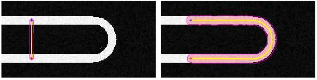
Isotropic model with P =√Pradius Anisotropic model with metric M
Fig. 10 Comparing segmentation results, on a synthetic “U” shape, when using isotropic and anisotropic models. Here, we took µ = 6.
4.2 Results on synthetic data
Our method is minimally interactive. First, the user has to decide if the desired vessels are darker or brighter than the background. So, we can consider different criteria on the signs of the eigenvalues. Then the scale range [rmin, rmax], which corresponds to
the range of radii of the vessel one wants to extract, is given by the user. In practice the user has to provide only the minimal radius value rminand the maximal one rmax.
Using the spatial image spacing, i.e hx, hy and hz, we chose a radius spacing equal
to 12min(hx, hy, hz) in order to respect the Nyquist sampling rate. Finally, few points
are required as source points or end points of the Fast Marching algorithm. We used the metric described in the previous section to find the minimal anisotropic path (as described in section 2) between two or more selected points (see figure 11). For any selected point, the associated initial radius is equal to the minimal radius rmin given
by the user.
Fig. 11 The red cross points are source points given by the user, and the blue ones are endpoints. On each case the segmented centerlines are displayed as well as the envelope of the moving discs. The associated minimal action map U as well as the 3D minimal path between the two selected points are shown (transparent visualization).
On figure 11, segmentation results on synthetic 2D images are shown. On the first synthetic image, the source point and destination are selected on the centerline. The obtained tube is perfectly detected as well as the centerline. On the second image, the initial points are not centered. But the centerline obtained by our algorithm goes back fast to the real centerline. This makes our algorithm robust to initialization. The third synthetic image shows that our approach is robust to scale changing.
On figure 12, we defined a cylinder on a 3D volume, with two different radii (4 and 6 voxels) on each half side of the volume. First, we tried our method with a reasonable anisotropy ratio, µ = 3, and by choosing the source and destination on the centerline of the desired tube. One can see that the desired tube is well segmented. Moreover,
Fig. 12 On the left, original synthetic tube with changing radii. We added 10% of salt and pepper noise. On the middle, selected source and destination are well centered. On the right, decentered initialization.
in figure 13 the evolution of the radius along the obtained minimal path shows that the radii are well detected. Also, we gave a bad initialization of the source and the destination for the second example of figure 12, and obtained a reasonable result.
0 200 400 600 800 1 2 3 4 5 6 7
Fig. 13 Evolution of the ra-dius along the obtained mini-mal path of figure 12 middle, when the points are well cen-tered along the desired tube.
µ = 3 µ = 5
Fig. 14 Influence of the maximal anisotropy ratio µ on the obtained minimal tube. For µ = 3 a shortcut occurs.
In order to challenge our method, we initialized the source and destination far from the desired tubular shape, in a situation for which a shortcut likely occurs, see figure 14. The original image used here is the synthetic volume of figure 12. One can see that for a reasonably small maximal anisotropy ratio µ, a shortcut occurs. While choosing a slightly higher value of µ allows us to overcome this problem.
Finally, on the example of figure 15 we designed a synthetic helix with linearly increasing radius (from 3 to 5 voxels). Similarly to the example of figure 14, we increased the value of the maximal anisotropy ratio µ to 5, in order to overcome the shortcut
0 50 100 150 200 0 1 2 3 4 5 6
Fig. 15 On the left, original synthetic helix with linearly changing radii. We added 10% of salt/pepper noise. On the middle, obtained segmentation. The blue line is the obtained centerline and the red one is the theoretic centerline. On the right, evolution of the radius along the obtained minimal path.
issue. The chosen radii range is [1, 6]. One can point out that the obtained centerline (the blue one) is slightly different than the theoretic one specifically near the source and the destination points. This is due to a boundary effect. Indeed, the source and destination are on the boundary of the volume and the computation of the OOF (on spatial or even on the Fourier domain) requires a special care for points near the boundary. For the spatial implementation of the OOF, when an image value for a point outside the domain is needed, we choose to use the nearest value on the domain. This choice has no effect on the orientation given by the OOF on the image of figure 12, while it can changes considerably the estimation of the vessel orientation for points in the vicinity of the domain boundary in general and particularly for the example given in figure 15. Also, on the same figure one can see the evolution of the radius along the obtained minimal path. Due to the voxelization, the radius evolution behaves almost like a piecewise constant function rather than a linear function.
4.3 Results on real images
In this section we are going to show some segmentation results on real images obtained by our method. For 2D images, see figure 16, we took a maximal anisotropy ratio µ = 5, and as said before, β is chosen such that the propagation speed along the radius dimension is at least twice the best propagation spatial speed. One can claim that our algorithm is robust to highly curved tubular structures, noise and bifurcations.
In figure 17, segmentation results are shown on real medical images. First, right coronary arteries (RCA) are segmented. Second, left anterior descending (LAD) ar-teries are segmented. One can see that the obtained radius on the principal coronary branches are larger than those of the secondary. Thus, our approach is robust to scale changing and bifurcations. The results presented here are encouraging but obviously not sufficient. A clinical validation is presented in the next section.
Fig. 16 On the left, original images. On the right, the red cross points are source points given by the user, and the blue ones are endpoints. On each case the segmented centerlines are displayed as well as the envelope of the moving discs.
Fig. 17 First line : RCA segmentation using the tubular anisotropy approach shown on the whole image and on the selected sub-volume. Second line : LAD segmentation shown on the whole image and on the selected sub-volume. Only few points are required (the extremities of the paths). The tubular anisotropy method provides the centerline as well as vessels boundaries.
4.4 Clinical validation
In order to make a genuine validation, we participated to “The Carotid Bifurcation Algorithm Evaluation Framework ”10which took place during a workshop of the MIC-CAI’09 conference [21]. The goal of this framework is to evaluate and compare different algorithms for carotid bifurcation, lumen segmentation and stenosis grading from CTA data.
The tubular anisotropy method proposed in this paper, represents vessels with cir-cular cross sections. This may yield various inaccuracies in the provided datasets, which contain vessels exhibiting non circular lumen and strong lumen occlusions. Therefore, we proposed to refine the segmentation using a region based level set model, see [47] for more details.
The competition data consists of CT angiography images acquired at the Erasmus MC, University Medical Center Rotterdam, The Netherlands (36 datasets), Hˆopital Louis Pradel, Bron, France (10 datasets) and the Hadassah Hebrew University Medical Centre, Jerusalem, Israel (10 datasets). The datasets have been selected such that they contain a large range of stenoses: from fully open to severe stenotic. Each hospital provided three points on the main branches of the carotid, for the whole data sets, and a manually drawn lumen segmentation for the training data sets, see [21] for more details.
Organizers of the competition proposed four performance measures: 1. the Dice similarity index Dsi
Dsi=
2 × |pvr∩ pvp|
|pvr| + |pvp|
,
where pvrand pvp are the reference and a participants partial volumes, the
inter-section operation is the voxelwise minimum operation, and |.| is the volume, i.e. the integration of the voxel values over the complete image.
2. the mean surface distance Dmsd,
Dmsd= 1 2× R Sr|sdmp|ds |Sr| + R Sp|sdmr|ds |Sp| ! ,
where sdmrand sdmp are the signed distance maps of the reference and a
partic-ipants segmentation, and Sr and Sp are the lumen boundary surfaces (isosurfaces
of the signed distance map at the value 0), and |Si| is the surface area of surface
Si, i.e. |Si| =RSids.
3. the root mean squared surface distance Drmssd,
Drmssd= 1 2× 0 @ sR Sr|sdmp| 2ds |Sr| + s R Sp|sdmr| 2ds |Sp| 1 A
4. maximum surface distance Dmax.
Dmax= 1 2× „ max x∈Sr |sdmp(x)| + max x∈Sp |sdmr(x)| « . 10 http://cls2009.bigr.nl/
All distance measures are symmetric, and all these measures are only evaluated in a the region of interest, see [21] for more details.
A summary of lumen segmentation scores is presented in Table 1. Averages lumen scores are presented in Table 2. The average processing time for a single data set was approximately 2 minutes. Our dice mean score is 83.6%, making our method relatively robust. Over nine teams that have participated to the contest, our method is fourth. As said previously, this might be explained by the fact that the Tubular Anisotropy method proposed in this paper detects vessels with circular cross sections yielding to inaccuracies on strong lumen occlusions. Moreover, for numerical reasons, we did not take advantage of the tubular anisotropy method by increasing as much as possible the anisotropy ratio µ. This point has been discussed in section 2.3.
Table 1 Summary lumen [47]
Measure % / mm rank
min. max. avg. min. max. avg. L dice 43.3% 93.6% 83.6% 3 4 3.97 L msd 0.20mm 3.98mm 0.80mm 3 4 3.97 L rmssd 0.29mm 6.50mm 1.57mm 3 4 3.97 L max 1.11mm 17.50mm 6.47mm 4 4 4.00
Total (lumen) 3 4 3.98
Table 2 Averages lumen [47]
Team Total dice msd rmssd max Total name success % rank mm rank mm rank mm rank rank TubularAnisotropy 31 83.6 4.0 0.80 4.0 1.57 4.0 6.47 4.0 4.0
ObserverA 31 95.4 1.5 0.10 1.5 0.13 1.6 0.56 1.9 1.6 ObserverB 31 94.8 2.4 0.11 2.4 0.15 2.3 0.59 1.8 2.2 ObserverC 31 94.7 2.2 0.11 2.2 0.15 2.1 0.71 2.3 2.2
5 Conclusion
In this paper we have proposed a new general method for tubular structure extraction in 2D and 3D images. Our method exploits the orientation of the vessels by using the optimally oriented flux to construct a multi-resolution anisotropic metric that ex-tracts from the image the local geometry and describes the vessels orientation and scales. Combining this metric with anisotropic minimal path technique, we were able to find a complete description of the tubular structure, i.e the centerline as well as the boundary. To summarize, our method is minimally interactive, robust to initializa-tion, scale variations, and bifurcations. Moreover, obtained clinical validation results are encouraging.
Acknowledgements
We would like to thank Professor Anthony J. Yezzi and Max Wai-Kong Law for fruit-ful discussions. Also Eduardo Davila for his precious help for the implementation of the first interface and Julien Mille for his collaboration for the carotid contest. This work was partially supported by ANR grant SURF-NT05-2 45825 and ANR grant MESANGE.
References
1. Fethallah Benmansour. Minimal Path Method applied to medical imaging: Tubular Struc-ture and Surface Segmentation using Multi-Scaled Anisotropy and Recursive Keypoints Detection. PhD thesis, Universit´e Paris Dauphine, 2009.
2. F. Bornemann and C. Rasch. Finite-element discretization of static Hamilton-Jacobi equa-tions based on a local variational principle. Computing and Visualization in Science, 9(2), 2006.
3. V. Caselles, R. Kimmel, and G. Sapiro. Geodesic active contours. In IEEE International Conference in Computer Vision (ICCV’95), pages 694–699, 1995.
4. V. Caselles, R. Kimmel, and G. Sapiro. Geodesic active contours. International Journal of Computer Vision, 22:61–79, 1997.
5. T. F. Chan and L. A. Vese. Active contours without edges. IEEE Transactions on Image Processing, 10(2):266–277, 2001.
6. S.-S Chern. Finsler geometry is just Riemannian geometry without the quadratic restric-tion. Not. Amer. Math. Soc., 43:959–963, 1996.
7. D. L. Chopp. Replacing iterative algorithms with single-pass algorithms. Proc Nat Acad Sc USA, 98(20):10992–10993, 2001.
8. L. D. Cohen and R. Kimmel. Global minimum for active contour models: a minimal path approach. International Journal of Computer Vision, 24:57–78, 1997.
9. Laurent D. Cohen and Thomas Deschamps. Segmentation of 3D tubular objects with adaptive front propagation and minimal tree extraction for 3D medical imaging. Computer Methods in Biomechanics and Biomedical Engineering, 10(4):289 – 305, August 2007. 10. Chris A. Davatzikos and Jerry L. Prince. An active contour model for mapping the cortex.
IEEE TMI, 14(1):65–80, March 1995.
11. T. Deschamps and L. D. Cohen. Fast extraction of minimal paths in 3D images and applications to virtual endoscopy. Medical Image Analysis, 5:281–299, 2001.
12. T. Deschamps and L. D. Cohen. Fast extraction of tubular and tree 3D surfaces with front propagation methods. In IEEE International Conference on Pattern Recognition (ICPR’02), pages 731–734, 2002.
13. Maxime Descoteaux, Louis Collins, and Kaleem Siddiqi. A geometric flow for segmenting vasculature in proton-density weighted MRI. Medical Image Analysis, 12(4):497 – 513, 2008.
14. E. W. Dijkstra. A note on two problems in connection with graphs. Numerische Mathe-matic, 1:269–271, 1959.
15. C. Lawrence Evans. Partial Differential Equations. American Mathematical Society, 1998. 16. A.F. Frangi, W.J. Niessen, K.L. Vincken, and M.A. Viergever. Multiscale vessel enhance-ment filtering. In lecture notes in computer science, volume 1496, pages 130–137. Springer-Verlag, 1998.
17. W. T. Freeman and E. H. Adelson. The design and use of steerable filters. IEEE Trans-actions on Pattern Analysis and Machine Intelligence, 13(9):891–906, 1991.
18. A. Gooya, H. Liao, K. Matsumiya, K. Masamune, Y. Masutani, and T. Dohi. A variational method for geometric regularization of vascular segmentation in medical images. IEEE Trans. on Image Processing, 17(8):1295–1312, August 2008.
19. Ali Gooya, Takeyoshi Dohi, Ichiro Sakuma, and Hongen Liao. Anisotropic Haralick edge detection scheme with application to vessel segmentation. In MIAR ’08: Proceedings of the 4th international workshop on Medical Imaging and Augmented Reality, pages 430–438, Berlin, Heidelberg, 2008. Springer-Verlag.
20. Ali Gooya, Takeyoshi Dohi, Ichiro Sakuma, and Hongen Liao. R-PLUS: A Riemannian Anisotropic Edge detection Scheme for Vascular Segmentation. In MICCAI ’08: Proceed-ings of the 11th international conference on Medical Image Computing and Computer-Assisted Intervention - Part I, pages 262–269, Berlin, Heidelberg, 2008. Springer-Verlag. 21. R. Hameeteman, M. Freiman, M.A. Zuluaga, L. Joskowicz, S. Rozie, M.J. van Gils,
L. van den Borne, J. Sosna, P. Berman, N. Cohen, P. Douek, I. Snchez, M. Aissat, A van der Lugt, G. P. Krestin, W.J. Niessen, and T. van Walsum. Carotid lumen segmentation and stenosis grading challenge. In Workshop in International Conference on Medical Image Computing and Computer Assisted Intervention, September 2009.
22. M. Hern´andez Hoyos, J. M. Serfaty, A. Maghiar, C. Mansard, M. Orkisz, I.E. Magnin, and P. Douek. Evaluation of semi-automatic arterial stenosis quantification. Int J Comput Assisted Radiol Surg, 1(3):167–175, 2006.
23. M. Holtzman-Gazit, R. Kimmel, N. Peled, and D. Goldsher. Segmentation of thin struc-tures in volumetric medical images. IEEE Transactions on Image Processing, 15:354–363, 2006.
24. in J. Tavares and R. Jorge. Advances in Computational Vision and Medical Image Pro-cessing: Methods and Applications, volume 13, chapter Geodesic Methods for Shape and Surface Processing, pages 29–56. Springer, 2009.
25. M. Jacob and M. Unser. Design of steerable filters for feature detection using Canny-like criteria. IEEE Transactions on Pattern Analysis and Machine Intelligence, 26(8):1007– 1019, August 2004.
26. S. Jbabdi, P. Bellec, R. Toro, J. Daunizeau, M. P´el´egrini-Issac, and H. Benali. Accurate anisotropic fast marching for diffusion-based geodesic tractography. J Biomed Imaging, 2008(1):1–12, 2008.
27. R. Kimmel and A. Bruckstein. Regularized Laplacian zero crossings as optimal edge integrators. International Journal of Computer Vision, 53:225–243, 2003.
28. Cemil Kirbas and Francis K. H. Quek. A review of vessel extraction techniques and algorithms. ACM Computing Surveys, 36:81–121, 2004.
29. E. Konukoglu, M. Sermesant, O. Clatz, J.-M. Peyrat, H. Delingette, and N. Ayache. A recursive anisotropic fast marching approach to reaction diffusion equation: Application to tumor growth modeling. In Proceedings of the 20th International Conference on Infor-mation Processing in Medical Imaging (IPMI’07), volume 4584 of LNCS, pages 686–699, 2-6 July 2007.
30. K. Krissian. Flux-based anisotropic diffusion applied to enhancement of 3-D angiogram. IEEE Trans. on Medical Imaging, 21(11):1440–1442, 2002.
31. Karl Krissian, Gr´egoire Malandain, and Nicholas Ayache. Directional anisotropic diffusion applied to segmentation of vessels in 3D images. In SCALE-SPACE ’97: Proceedings of the First International Conference on Scale-Space Theory in Computer Vision, pages 345–348, London, UK, 1997. Springer-Verlag.
32. Max W. Law and Albert C. Chung. Three dimensional curvilinear structure detection using optimally oriented flux. In ECCV ’08: Proceedings of the 10th European Conference on Computer Vision, pages 368–382, Berlin, Heidelberg, 2008. Springer-Verlag.
33. Max W.K. Law and A.C.S. Chung. Weighted local variance-based edge detection and its application to vascular segmentation in magnetic resonance angiography. IEEE Transac-tions on Medical Imaging, 26(9):1224–1241, September 2007.
34. W. K. Law and Albert C. S. Chung. Segmentation of vessels using weighted local variances and an active contour model. In CVPRW ’06: Proceedings of the 2006 Conference on Computer Vision and Pattern Recognition Workshop, page 83, Washington, DC, USA, 2006. IEEE Computer Society.
35. Christophe Lenglet, Emmanuel Prados, Jean-Philippe Pons, Rachid Deriche, and Olivier Faugeras. Brain connectivity mapping using riemannian geometry, control theory and pdes. SIAM Journal on Imaging Sciences (SIIMS), 2(2):285–322, 2009.
36. David Lesage, Elsa D. Angelini, Isabelle Bloch, and Gareth Funka-Lea. Bayesian maximal paths for coronary artery segmentation from 3d ct angiograms. In Guang-Zhong Yang, David J. Hawkes, Daniel Rueckert, J. Alison Noble, and Chris J. Taylor 0002, editors, International Conference on Medical Image Computing and Computer Assisted Interven-tion, (1), volume 5761 of Lecture Notes in Computer Science, pages 222–229. Springer, 2009.
37. David Lesage, Elsa D. Angelini, Isabelle Bloch, and Gareth Funka-Lea. A review of 3D vessel lumen segmentation techniques: Models, features and extraction schemes. Medical Image Analysis, 13(6):819–845, August 2009.
38. H. Li and A. Yezzi. Vessels as 4D curves: Global minimal 4D paths to extract 3D tubular surfaces. In IEEE Conference on Computer Vision and Pattern Recognition (CVPR’06), Workshop MMBIA06, page 82, 2006.
39. H. Li and A. Yezzi. Vessels as 4-D curves: Global minimal 4-D paths to extract 3-D tubular surfaces and centerlines. IEEE Transactions on Medical Imaging, 26(9):1213–1223, 2007. 40. Qingfen Lin. Enhancement, extraction, and visualization of 3D volume data. PhD thesis,
Linkopings Universitet, 2003.
41. Tony Lindeberg. Edge detection and ridge detection with automatic scale selection. In-ternational Journal of Computer Vision, 30:465–470, 1998.
42. P. L. Lions. Generalized solutions of Hamilton-Jacobi equations. Pitman, Research Notes in Mathematics, 69, Boston-London-Melbourne, 69, 1982.
43. Cristian Lorenz, I.-C. Carlsen, Thorsten M. Buzug, Carola Fassnacht, and J¨urgen Weese. Multi-scale line segmentation with automatic estimation of width, contrast and tangential direction in 2D and 3D medical images. In CVRMed-MRCAS ’97: Proceedings of the First Joint Conference on Computer Vision, Virtual Reality and Robotics in Medicine and Medial Robotics and Computer-Assisted Surgery, pages 233–242, London, UK, 1997. Springer-Verlag.
44. R. Manniesing, M. A. Viergever, and W. J. Niessen. Vessel axis tracking using topology constrained surface evolution. IEEE Transactions on Medical Imaging, 26(3):309–316, 2007.
45. R. Manniesing, M. A. Viergever, and W.J. Niessen. Vessel enhancing diffusion: A scale space representation of vessel structures. Medical Image Analysis, 10(6):815–825, 2006. 46. J. Melonakos, E. Pichon, S. Angenent, and A. Tannenbaum. Finsler active contours. IEEE
Trans. Pattern Analysis and Machine Intelligence, 30(3):412–423, March 2008.
47. Julien Mille, Fethallah Benmansour, and Laurent D. Cohen. Carotid lumen segmentation based on tubular anisotropy and contours without edges. In Insight Journal, 2009. 48. Vandana Mohan, Ganesh Sundaramoorthi, John Melonakos, Marc Niethammer, Marek
Kubicki, and Allen Tannenbaum. Tubular surface evolution for segmentation of the cingu-lum bundle from DW-MRI. In Mathematical Methods in Computational Anatomy, 2008. 49. Delphine Nain, Anthony Yezzi, and Greg Turk. Vessel segmentation using a shape driven flow. In Medical Imaging Copmuting and Computer-Assisted Intervention (MICCAI’04), pages 51–59, 2004.
50. O. Nemitz, M. Rumpf, T. Tasdizen, and R. Whitaker. Anisotropic curvature motion for structure enhancing smoothing of 3D MR angiography data. Journal of Mathematical Imaging and Vision, 27(3):217–229, April 2007.
51. Maciej Orkisz, Leonardo Fl´orez Valencia, and Marcela Hern´andez Hoyos. Models, algo-rithms and applications in vascular image segmentation. Mach Graph Vision, 17(1):5–33, 2008.
52. E. Rouy and A. Tourin. A viscosity solution approach to shape from shading. SIAM Journal on Numerical Analysis, 29:867–884, 1992.
53. Y. Sato, S. Nakajima, N. Shiraga, H. Atsumi, S. Yoshida, T. Koller, G. Gerig, and R. Kiki-nis. Three-dimensional multi-scale line filter for segmentation and visualization of curvi-linear structures in medical images. Med Image Anal, 2(2):143–168, 1998.
54. J. A. Sethian. A fast marching level set for monotonically advancing fronts. Proceedings of the National Academy of Sciences, 93:1591–1595, 1996.
55. J. A. Sethian and A. Vladimirsky. Fast methods for the eikonal and related Hamilton-Jacobi equations on unstructured meshes. Proceedings of the National Academy of Sci-ences, 97(11):5699–5703, May 2000.
56. Kaleem Siddiqi and Alexander Vasilevskiy. 3d flux maximizing flows. In EMMCVPR ’01: Proceedings of the Third International Workshop on Energy Minimization Methods in Computer Vision and Pattern Recognition, pages 636–650, London, UK, 2001. Springer-Verlag.
57. Ganesh Sundaramoorthi, Anthony Yezzi, Andrea C. Mennucci, and Guillermo Sapiro. New possibilities with sobolev active contours. Int. J. Comput. Vision, 84(2):113–129, 2009. 58. J. N. Tsitsiklis. Efficient algorithms for globally optimal trajectories. IEEE Trans.
Au-tomat. Contr., 40:1528–1538, 1995.
59. Ofir Weber, Yohai S. Devir, Alexander M. Bronstein, Michael M. Bronstein, and Ron Kimmel. Parallel algorithms for approximation of distance maps on parametric surfaces. ACM Trans. Graph., 27(4), 2008.
60. Joachim Weickert. Coherence-enhancing diffusion filtering. Int. J. Comput. Vision, 31(2-3):111–127, 1999.