Urban Poverty Dynamics in Peru and Madagascar 1997-1999: A Panel Data Analysis
Javier Herrera*, François Roubaud**
Abstract
The limits of the welfare-type anti-poverty policies promoted in the eighties in order to counter the effects of structural adjustments programs (SAP) have led to an awareness of the need to reflect on interactions among anti-poverty programs and, more importantly, to conceive and put in place anti-poverty policies adapted to the different existing types of poverty, as well as to draw attention to the factors associated to exits from poverty.
However, the small number of studies on poverty dynamics in developing countries and methodological differences among them have made it difficult to identify what the implications are for anti-poverty policies. Are the factors associated to chronic poverty and vulnerability the same from one country to the next? What are the features that characterize exits from poverty?
Based on a large sample of Peruvian and Madagascan urban households (1997-1999), the importance of poverty transitions was examined, as well as the characteristics of the temporarily and the chronically poor, with respect to those of non-poor households. Then, through a multinomial logit model, the specific contribution of household characteristics (demographics, human and physical capital), but also of shocks –related to both demographics and job market– experienced by these households, on chronic poverty and poverty entries and exits was highlighted. In this analysis, the impact of « geographic » variables linked to neighborhoods (provision of public goods, income levels, human capital and employment structure, among others) on poverty transitions was also considered. The two latter groups of variables are rarely considered in empirical research on developing countries (shocks are set aside in analyses because of the simultaneity biases that exist when no more than two years of observation are available). Result comparability was ensured by defining the variables and formulating the econometric model in a rigorously identical manner in both countries.
The factors associated to permanent poverty amply cover the characteristics generally identified in analyses on « static » poverty correlates. Nevertheless, these results do not confirm the idea that only shocks are relevant to temporary forms of poverty. The type and quality of entry on the job market, as well as the features of the residence neighborhood, turn out to be equally relevant in the analysis of poverty dynamics. These results suggest that the spatial « inequality » dimension should be added to analyses on income and poverty transition dynamics.
Themes : welfare, poverty, income distribution
Keywords : poverty dynamics, inequality, Peru, Madagascar, multinomial logit, panel data JEL: I32, D63, D31
*
Researcher at IRD-INEI, UR 047 , CIPRE; E-mail: [email protected]
2 Introduction
In recent years, the fight against poverty has become the main objective of development policies. The mixed results produced by two decades of stabilization and structural adjustment on the standard of living of households in developing countries have led the international financial community, encouraged by the Bretton Woods Institutions, to rethink its strategy and develop new instruments to conduct what has now taken the shape of a real crusade. The Economic Policy Framework Papers (EPFP), which defined the accessibility conditions to financial assistance to development agencies are now titled Poverty Reduction Strategy Papers (PRSP). The World Bank’s traditional « Structural Adjustment Credit » (SAC) has been replaced with the « Poverty Reduction Support Credit » (PRSC). Even the IMF, which had been rather uninvolved on that front, has followed suit by transforming its « Enhanced Structural Adjustment Facility » (ESAF). A new debt reduction mechanism was introduced to complement prior debt write-off and rescheduling agreements (Paris Club; Toronto, Naples, Lyon Terms; etc.) through the Heavily Indebted Poor Countries (HIPC) Initiative. To signal their commitment, the main donors have set eight Millenium Development Goals (MDG), the first of which is to reduce the incidence of extreme poverty by half from 1990 to 2015. Although the priority of the fight against poverty is focused, above all, on the least developed countries, it also concerns middle-income countries, in order to include all developing and transition countries.
This new direction in development policy poses a formidable challenge for the scientific community, and economists in particular, as shown by the World Bank in its report on world development titled, « Attacking Poverty » (World Bank, 2000). The objective of the present study is to contribute to this vast reflection by means of a comparative analysis of individual poverty dynamics in two developing countries, Madagascar and Peru, in the late nineties. The interest of this research lies in a rigorous comparison of the factors that determine poverty transitions, based on two panels of urban households, over a three-year period, in two very different contexts. The first case looks at one of the poorest countries in the world as it finds itself in a phase of rapid recovery, and the second, an at an emerging country engaged in a recession.
Judgements on the disappointing progress made in the fields of living standards and international inequalitiy are generally founded on a static perspective, based on comparing the indicators of a given year to those of past years. Only net poverty balances are considered, but households’ trajectories over time are ignored. Conclusions drawn from static approaches on whether or not poverty persists imply that the poor constitute a set category of households with the same specific features and permanent in nature. This therefore implies that there is no (or little) income redistribution to the benefit of the lowest segments of income distribution.
Monitoring a panel of households allowed addressing important questions, which had remained unanswered in Developing Countries until then. What proportion of the population is in a situation of chronic poverty? In a given year, what percentage of the poor corresponds to transient poor? What is the significance of the economic mobility of households and, particularly, between poor and non-poor? Do the permanent poor display characteristics different from those of the transient poor ? Are the factors that determine entry into poverty the same as those that determine exit from it? What are the changes in the features of households and their environment that are associated with upward and downward mobility? How does this dynamic approach to poverty lead to a reconsideration of anti-poverty policies and an assessment of their efficiency? Few developing countries are equipped to tackle these issues, as this involves conducting large-scale monitoring of the same households over time, and such surveys are extremely rare in these countries.
The different forms of poverty that exist may be understood more subtlety through the study of the features and determining factors of poverty and non-poverty, especially by distinguishing between the chronically poor and the temporarily poor and, hence, result in the implementation of differentiated policies linked to the specific risk factors of each of the two categories. This would be quite apart from targeting problems (« filtering » and « exclusion ») due to a high degree of social mobility between poverty and non-poverty.
Although abundant in developed countries, the literature on the issue of economic mobility and poverty dynamics based on panels of households (for example, see Jenkins, 1998) remains very scarce in developing countries. The main reason for this is the lack of longitudinal data. Yacub (1999) stated that only 5 of the 44 low human development countries, and 7 of the 66 countries with intermediate human development, according to the UNDP classification, had available panel data. In a recent publication on the issue, Baulch and Hoddinot (2000) confirmed this panel data shortage. The book they edited, which includes 6 original studies (Ethiopia, South Africa, China, Pakistan, Zimbabwe and Chile), constitutes the first attempt to draw lessons from this type of approach. However, the extreme diversity of the panels used (in terms of geographic extension, reference timeframe, type of sampling, welfare indicators, poverty line, etc.) considerably limits the analytical scope of these different case studies, particularly with respect to their comparison dimension.
Following the same thematic line, the present article constitutes, to our knowledge, the first attempt at a comparative analysis of poverty dynamics, based on a shared methodological approach and the same choices. By mobilizing two high-quality panels and adopting homogenous procedures for constructing analytical variables, the best
3 conditions are achieved to conduct a study of the risk factors for entering poverty and those associated with chronic poverty. The issue is therefore to find out if the level of development and the existing economic situation affect the intensity of poverty « flows » In addition, the fact that the study was conducted over three consecutive years allowed the inclusion of shocks on households (demographic and economic) among variables that explain poverty transitions, while preventing endogeneity problems that cannot be solved when only two points in time are available. Finally, we have attempted to broaden the field of factors that explain poverty transitions by adding variables associated with residence neighborhoods to the traditional individual features of households, in order to assess the possible effects of geographic location on poverty.
The macroeconomic context in place during the three-year period of the study (1997-1999) is introduced in the first section by examining the period in a historical perspective, as well as the main features of the data used and the methodological choices made. A summary of the evolution of poverty and inequality by means of a cross-section analysis is the subject of the second section. An estimate of confidence intervals and analysis in terms of stochastic dominance confirm the robustness of the results based on comparing traditional FGT indexes. A growth/inequality decomposition of the evolution of poverty has also been carried out. The third section focuses on a descriptive analysis of poverty transitions, which are modeled in the fourth section. Finally, the concluding section provides a summary of the study’s main results and examines some of their implications regarding policies designed to fight poverty.
I.- General Overview
The macroeconomic context of the nineties
Despite very different development levels – the per capita GDP of Peru is ten times that of Madagascar (US $2 400 and US $250, respectively–, both countries applied very similar policies in the nineties. Following the failures of past economic policies and, as many developing countries did, both Peru and Madagascar attempted to redirect their growth model by banking on the liberalization of the economies and opening to the world economy. The change was adopted as early as the mid-eighties in Madagascar, while it waited until 1990 to come about in Peru, when president Fujimori came to power.
Peru
The nineties were years of profound institutional reforms and macroeconomic shocks that broke with the previous regime based on political favors, whose economic « heterodoxy » had plunged the country into chaos (hyperinflation, etc.). While most public and parapublic corporations were being privatized, and subsidies and price controls eliminated, the government carried out unprecedented labor market reforms. Job stability was practically abolished and dismissal costs greatly reduced. Financial incentives convinced 150 000 public employees to leave their jobs, while, simultaneously, labor market deregulation resulted in the spread of precarious work. In this context, the proportion of stable jobs in the capital dropped from 65% in 1989 to 42% in 1994, and to 23% in 1997 (Vedera, 2000). Over the same period, the rate of unionization plummeted: from 58% in 1989, it fell to under 13% in 1997.
After the first phase of the harsh recession that followed the « Fujishock » (the GDP lost 5% in 1990), Peru underwent a period of vigurous expansion from 1993 to 19971. Its GDP per capita grew by more than 6% annually. However, since the second half of 1997, Peruvian economic growth has slowed down sharply, and became negative following the Asian crisis, as happened in most Latin American economies. The short-term capital inflow dried up and main export prices fell, which was compounded by the devastating effects of El Niño. In the end, when examined from a long-term perspective, the GDP leap of more than 50% observed under president Fujimori’s administration has only resulted in a return to the level reached in 1972.
In 1998 and 1999, the Peruvian GDP per capita registered drops of 2,1% and 0,3%. The dualism of the Peruvian economy, in which growth is driven by a dynamic primary-products export sector, has hidden the magnitude of the crisis for households, who suffer first and foremost from domestic market shrinkage. Per capita private consumption fell by 2,7% in 1998 and 1,9% in 1999, after having grown 2,4% under the impulse of resumed public spending during the previous year, which had risen 7,6% that year. Household survey results confirmed the extent of the decline in consumption registered in national accounts, in which real per capita spending dropped 8% between 1997 and 1999.
Such a downturn in economic activity meant a worsening unemployment rate (from 7,2% to 9% between 1996 and 1999), even though it was not readily affected by macroeconomic shocks (mostly due to the absence of unemployment insurance and to a high proportion of independent informal workers). Workers’ wages in companies employing over 10 workers decreased by 0.5% from 1997 to 1998, and by 1,3% the following year. The decline in
1 Interestingly, the final years of the government of Alan García did far more harm to economic growth than the "Fujishock": between 1987 and
4 living standards is shown indirectly by the strategies households used to counter the crisis. Hence, the participation rate in the capital city has gone from 59,7% in 1996 to 64% in 1999.
In this unfavorable context, the incidence of poverty at the national level significantly increased from 1998 to 1999 (from 37,7% to 42,2%)2. Poverty became more urban as three quarters of the increase in the number of poor people was concentrated in urban areas. The poverty rate rose 7 points in the capital and on the coast, whereas it remained stable in rural regions. Between 1997 and 1999, 43% of the one and a half million additional poor people were from the capital and 30% from coastal cities. By contrast, the incidence of extreme poverty declined by 15,6% to 13,2% between 1997 and 1999, thanks especially to a 10 point decrease in its incidence in rural regions, while it stayed relatively stable in urban areas. The contrasting evolution of poverty in different areas was certainly not unaffected by the reform policies implemented. These were more likely to have an effect on the modern and urban sector of the economy. At the same time, the government launched a program to fight poverty and initiated an unprecedented increased social spending, which tripled from 1993 to 1998, from US $63 to US $174 per capita, and was largely directed to the country’s poorest rural regions.
Table 1
Madagascar and Peru in numbers (1999)
Madagascar Peru Madagascar Peru
Area (1 000 km2)
587 1 285 GDP (billions US$) 3,7 51,9
Population (millions) 14,6 25,2 GDP per capita (US$) 250 2 130 Population growth rate (%) 2,8 1,7 Investment rate (% GDP) 12 22
Urban population (%) 29 72 Tax burden (% GDP) 11 12
Life expectancy (years) 58 69 Foreign debt (% GDP) 123 61
Madagascar
For nearly 15 years, Madagascar has been engaged in a process of economic adjustment. Although the first phase focused on financial stability, the limits of the policy quickly came to light. The second phase intended to establish in-depth changes in the economic regulation mode. Regardless of hesitations, the authorities undertook a wide range of reforms to promote a market economy. Among the measures taken were:
- the elimination of export taxes;
- a significant decrease in import duties and taxes;
- the liberalization of marketing channels and previously administered prices; - the establishment of a regime of free export companies;
- the application of a floating exchange rate;
- government disengagement from production activities, particularly from the banking sector.
Even though difficulties in pursuing sectorial reforms persisted in certain areas (public corporation privatization, public service reform, etc.), the progress made reflected an advanced degree of commitment in the process of establishing a market economy opened to the outside world. In fact, since the early nineties, Madagascar has carried out a double transition: economic, of course, but also political. The country successfully scrapped a two-decade, socialist-type experiment in favor of a democratic regime (free elections, freedom of the press, emerging civil society, etc.). Strengthened by such progress, Madagascar reestablished ties with the international financial community in 1996 and was allowed to benefit from numerous loans and debt write-offs (SAC, ESAF, Paris Club, etc.)
However, despite the magnitude of the reform program, the Madagascan economy stagnated during the first half of nineties. The ongoing political instability that prevailed over that period was largely to blame for this growthless adjustment phase. It was finally only in 1997 that the recovery began to be felt: for the first time in many years, the GDP per capita improved slightly (+1%). Since then, the process has quickened, and growth neared 5% in 2000. This bright spell is exceptional in Madagascar’s economic history. To find such a favorable situation, one must go back to the sixties. Inflation is now under control, following its spiraling in 1994-96, which had been generated by exchange rate liberalization. Although overall, the integration of Madagascar within the world economy has not substantially improved, due to the inertia of traditional primary-products exports and the stagnation of external private capital flow, a few sectors have managed relatively well. This is the case of tourism, fishing and, most importantly, the industrial duty-free export processing zone, where exceptional dynamism contrasts with the slump that characterizes Madagascar’s counterparts in sub-Saharan Africa (except for Mauritius).
The macroeconomic evolution displayed by data from the country’s national accounts does not adequately reflect household income dynamics, mostly because of their poor quality. Suveys conducted with households showed an unprecedented boom in the urban economy, whereas rural areas stagnated. In cities, informal jobs, which had progressively taken over the labor market were in decline, while real wages and households’ per capita income registered increases of 43% and 35%, respectively, from 1995 to 1999 (Razafindrakoto, Roubaud, 1999). This exceptional improvement, which benefited every household category, was spurred by a very generous policy of public
2
Both for Peru and Madagascar, poverty levels mentioned in this section agree with official data. They do not compare with those calculated in the rest of the study due to different data sources and methodological choices (geographic coverage, poverty line, income versus consumption, etc.).
5 and private wages. On the other hand, rural regions, massively excluded from the market, did not benefit from returns on growth. Such dualism generated rising inequalities between urban and rural areas, as pockets of poverty are massively concentrated in the countryside (84% of the poor).
The evolution of poverty has followed households’ income fluctuations. According to the results of EPM surveys conducted in 1993, 1997 and 1999, the incidence of poverty at the national level slightly decreased from 1997 to 1999 (-2 points). However, this global observation conceals different dynamics in urban and rural areas. While levels of rural poverty remained high (76% and 76,7%), they declined by over 11 points in the cities (63,2% and 52,1%). In both cases, the incidence of poverty was always above that registered in 1993 (Razafindravonona, Stifel, Paternostro, 2001). From a longer-term point of view, households’ standards of living remained far below those observed in the early seventies, since, between 1971 (the best year) and 1996 (when the lowest point was reached), per capita consumption fell by half. In the case of the capital city, where data has been available since independence, the standard of living was seen to have dropped by 30% from 1961 to 1998 (Ravelosoa, 2001). The impact of specific policies to fight poverty (transfers, social spending, etc.) remained marginal due to insignificant budgetary allocations (the tax rate could hardly reach 10% of the GDP).
Figure 1
Per capita GDP Evolution 1960-2000
60 70 80 90 100 110 120 130 140 150 M adagascar Peru 1960=100
Sources: INSTAT, Madagascar, Banco Central de Reserva (Central Reserve Bank), Peru, authors’ calculations.
The Data
In order to carry out the analysis of individual poverty transitions, panel data was required. In addition, the comparative perspective adopted here implied that the surveys and processing procedures has to be harmonized. Both these constraints explain why, to our knowledge, no such research had previously been conducted. The data used are briefly introduced below, as well as the main methodological options chosen.
ENAHO research in Peru
In 1996, with the support of the Inter-American Development Bank, the Peruvian National Statistics and Data Processing Institute (INEI) set up a system of household surveys (ENAHO), as part of the MECOVI Program. Through these surveys, the population’s living conditions, among other things, could be monitored. The constitution of a large national panel of households was one of the major innovations of this Program. Besides their national coverage, the surveys allowed the decomposition of results according to seven geographic domains, in addition to the distinction between urban and rural areas. Four quarterly surveys were involved, each focusing on a specific issue (violence, employment, health, education, household expenditures). In the present case study, only waves in the last quarter of each year have been used, as they are the only ones with a panel dimension.
The panel on hand was composed of 1720 urban households and of almost 8 000 individuals present every year over the 1997-99 period. Two biannual sub-panels, made up of 2709 households in 1997-98 and 1872 households in 1998-99, were also available. The households present in the panel for all three consecutive years represented a little over 40% of the total in 1997 and 1998, and nearly 78% in 1999. In addition to the information on individuals’ housing and demographic features, the surveys included sections on education, health, expenditures, income, employment, etc.
6 The MADIO Employment Survey in Madagascar
Since 1995, the National Statistics Institute (INSTAT), with the support of the MADIO Project, had run a 1-2-3 household survey system in the city of Antananarivo (Roubaud, 2001; Rakotomanana, Ravelosoa, Roubaud, 2001). It was based on an employment survey (phase 1), carried out every year, on a sample of 3000 households and approximately 15 000 individuals. This survey was the basis of phases 2 (informal sector) and 3 (consumption, poverty), conducted every three years (1995, 1998, 2001), according to the survey-grafting principle. In 2000, the survey was extended to the country’s 7 largest cities. It must be underlined that such a mechanism was unheard of in sub-Saharan Africa. Specifically, since strict control procedures were used at every step (collecting, screening, processing), the quality of the Madagascan data was by far superior to that found in most household surveys in Africa.
The results analyzed in this paper were taken from 1995-2000 employment surveys. They specifically include the 1997-99 panel data. In fact, since 1997, the principle of renewing a third of the sample each year (that is 1000 households) has been adopted. Nonetheless, taking into account the loss observed between 1997 and 1998, the total 1998 sample was surveyed in 1999. Finally, the 1997-99 panel was based on a usable sample of 2 676 households: 1 551 surveyed in 1997 and 1998, and 2 371 in 1998 and 1999, including 1249 for which data was available over the three years of the study. Because information was gathered individually from all household members, 13 539 individuals belonging to 2 676 households were involved: 8 149 in 1997 and 1998, and 12 138 in 1998 and 1999, including 6 478 over the three-year period. Besides the traditional socio-demographic data and housing features, the survey addressed the individuals’ situation vis-à-vis the labor market (inactivity, unemployment, job type), as well as income. Tableau 2 Samples used 1997-1999 Madagascar Peru Number of households 1997 1998 1999 1997 1998 1999 Total Sample 3 000 3 002 3 002 4 022 4 044 2 218 1997-1998 Panel 1 551 1 551 - 2 709 2 709 - 1998-1999 Panel - 2 371 2 371 - 1 872 1 872 1997-1998-1999 Panel 1 249 1 249 1 249 1 720 1 720 1 720
Sources: Employment surveys 1997-1999, MADIO, Enaho 1997-1999, INEI, authors’ calculations. Measuring Welfare and Constructing Poverty Lines
Unlike in many studies, welfare levels and the monetary poverty measurements derived from them are based on the per capita income of households. This choice responded chiefly to the need to be able to compare both countries –expenditure estimates for the Madagascan panel were not available–, but was also founded on a certain number of analytical considerations. First, the argument often put forth to favor the approach that refers to expenditure instead of income is based on the idea that, in surveys, the former is grasped better than the latter. This argument did not seem systematically justified to us and is probably quite overestimated. Nothing ensured that errors in consumption measurement (valorization of self-consumption, complexity of consumption reconstituting procedures over a year, memory effect, etc.) were fewer than errors in income3. In fact, this observation was corroborated in the case of developed countries (Verger, 2001). It led Verger to conclude that, "In the end, it is not easier to measure expenditures than income: it may even be more difficult and one must recognize that the individual consumption distribution drawn from surveys on household budgets has hardly any value at all at the individual level, and could not provide the basis for an approach on inequalities or poverty." This is the reason why, in Europe, poverty measurements are based on income rather than expenditures.
Second, since the objective of the study was to link macroeconomic shocks to changes in households’ living standards over a short period, the use of the consumption variable –often interpreted as a measure of permanent income– did not seem the most appropriate. On the other hand, income seemed more closely connected to existing conditions on the labor market, which was also under the direct influence of the macroeconomic situation. Furthermore, in terms of economic policy, it is easier to act on income than on consumption, since the later is actually only a result of the former. Finally, the fact that we limited the field of our study to urban households also ensured that exogenous shocks due to the weather were minimized. In fact, in late 1997, the El Niño phenomenon severely affected agricultural activities in Peru. Both entries into poverty (in 1998) and exits from poverty (in 1999) in rural areas are associated to the fall and subsequent recovery of agricultural production due to that natural phenomenon, in proportions difficult to assess. This is obviously much less common in the case of urban income, which is more closely linked to the evolution of the domestic market.
The "income" variable used in this study corresponded to the sum of all incomes (monetary and non-monetary) of each household member, except for capital income. They included wages from work in the main and secondary,
3 For example, the consumptopn of households involved in the 1993 survey in Madagascar represented only one third of private consumption in the
7 formal and informal activities, as well as benefits in kind, social assistance benefits and pensions. Although not including capital income introduced a bias in the measurement of total income, this was not a priori likely to affect the results obtained, due to the little weight they have in developing countries, particularly among the poor. To establish inter-temporal and geographic comparisons, we adopted an absolute poverty line common to both countries. According to classic works in this field (Ravallion, 1996), the threshold used corresponded to the amount needed to achieve a food consumption norm of 2 300 calories per capita, per day, to which a complementary amount was added for non-food expenses. Calculated for 1998, when consumption surveys were available for both countries, these lines were retropolated and extrapolated using the corresponding consumer price index, that is, 140 300 Madagascan francs and 198 new soles, respectively, equivalent to 2 and 4 current dollars.
From the start, both panels were systematically controlled and outliers eliminated. In addition, the study of attrition biases ensured that the panels used were good-quality panels and represented well the reality to be examined in both countries. Finally, in order to be able to make a comparison, only variables common to both series of surveys were used in the analysis. These variables were constructed by using strictly identical definitions and calculation methods.
II.- Poverty, Growth and Inequalities in the Second Half of the Nineties
Urban Poverty Evolution and Levels (1995-2000)
From 1995 to 2000, poverty fell over 12 points in the Madagascan capital. It was reduced from 86% to 74%. 1997 and 2000 were the two best years in this regard. This decline was not limited to the incidence of poverty, but also affected FGT indicators, particularly poverty gap and severity (P1 et P2), for which it was even more spectacular (-16 points in 5 years). This considerable drop was all the more significant because it constituted an actual trend reversal, as poverty had continuously increased over a long period of time, that is, at least since the early seventies. Despite such improvement, in 2000, nearly three out of four residents of the capital, Antananarivo, were still poor. In the case of Peru, the trend is not as clear. Following a sharp, 6-point decrease between 1994 and 1997, poverty levels stabilized during the next period (1997-1999). Neither the slight, 2-point decline observed between 1997 and 1998, nor the upturn the following year are statistically significant.
In terms of levels, the comparison of both countries’ urban poverty incidence sheds a bright light on the gap between the two. There was a 50-point difference in the mid-nineties. In spite of the exceptional dynamism of the Madagascan economy, the gap still reached 47 points in 1999. At such a pace, twenty years will be required for Madagascar to equal the standard of living currently registered in Peru.
Table 3
Evolution of Monetary Poverty, 1995-2000
Madagascar Peru 1995 1996 1997 1998 1999 2000 1994 1997 1998 1999 P0 85,8 [82,6-89,0] 85,6 [82,9-88,2] 80,5 [78,1-83,0] 79,6 [77,3-81,8] 77,3 [74,8-79,9] 73,6 [70,3-76,8] 35,9 [32,6-39,3] 30,2 [27,8-32,5] 28,6 [25,7-31,5] 30,3 [27,2-33,5] P1 52,5 [49,1-55,8] 50,7 [48,1-53,2] 44,7 [42,7-46,7] 44,3 [42,2-46,4] 42,6 [40,5-44,7] 36,1 [33,6-38,7] 12,5 [10,9-14,0] 10,4 [9,4-11,3] 10,4 [8,9-11,8] 10,2 [8,8-11,6] P2 36,7 [33,7-39,7] 34,8 [32,6-36,9] 29,3 [27,6-30,9] 29,3 [27,5-31,1] 28,1 [26,3-29,9] 21,8 [19,8-23,8] 6,0 [5,1-6,9] 5,1 [4,5-5,6] 5,4 [4,4-6,3] 5,2 [4,1-5,8] Sources: Employment surveys 1995-2000, MADIO, Enniv 1994, Enaho 1997-1999, authors’ calculations. 5% confidence intervals in parentheses
The study of the evolution of extreme poverty –the threshold of which corresponds to a subsistence food basket– confirms the diagnosis presented above. In 1995, 61% of Antananarivo’s residents lived in this situation of extreme hardship. However, the proportion of the extremely poor continued to decrease, reaching 39% in 2000. The gap and severity of extreme poverty followed similar trends: they fell by half over the same period (from 30 to 15% for P1 and 18 to 8% for P2). In Peru, no change occurred between 1994 and 1999. The incidence of extreme poverty was about 9%, 3% gap and a little over 1% severity. Toward the end of the period, the incidence of extreme poverty remained 5 times higher in Madagascar than in Peru.
Juxtaposing income distributions per capita (expressed in real terms) provides a graphic view of the evolution in progress. In particular, it relaxes the constraints imposed by the choice of a poverty line, which is arbitrary by nature. Figure 2 clearly illustrates the decline of poverty in both countries. For Madagascar, the curves shift toward the right from one year to the next (except in 1995 and 1996, where they intersect), especially in the area between the thresholds of extreme poverty (lower limit) and poverty (upper limit). In the case of Peru, two distinct groups of years are visible: 1994, when the situation was the least favorable, and 1997-99, when the relative position of the distributions varied according to the considered line.
8 Figure 2
Income Distributions Per Capita, 1995-2000
Sources: Employment surveys 1995-2000, MADIO, Enniv 1994, Enaho 1997-1999, authors’ calculations.
An analysis in terms of stochastic dominance, based on the above distribution comparison, tested the robustness of the conclusions drawn above, regardless of the poverty line chosen. In Madagascar, the analysis confirmed the substantial decline of poverty over the entire period. At the 5% threshold, Kolmogorov-Smirnov tests show that, every year, income distribution per capita "dominates" that of the previous year, with the sole exception of 1997 and 1998, when the hypothesis of equal distributions cannot be rejected. In other words, the incidence of poverty decreased systematically, in a statistically significant manner, from one year to the next, regardless of the poverty line chosen. The disconnection observed in 1997 and 2000 with respect to the incidence of poverty is found over the entire income distribution. Improvements in the situation of households actually affected all living conditions, whether assessed from a monetary (income, consumption) or non-monetary (housing comfort, access to public services, schooling, etc.; Razafindrakoto, Roubaud, 1999) point of view. In Peru, the conclusions are more ambiguous. Although the 1994 distribution is significantly "dominated" (by 5%) by those of 1997-1999, which means that the incidence of poverty declined, the diagnosis over the three years cannot distinguish them.
Table 4
Evolution of Poverty: First Order Stochastic Dominance Tests, 1995-2000 Madagascar Peru 1994 1995 1996 1997 1998 1999 2000 1994 - - - 1995 - - M M M M M 1996 - - - M M M M 1997 P - - - ns M M 1998 P - - ns - M M 1999 P - - ns ns - M 2000 - - -
Sources: Employment surveys 1995-2000, MADIO, Enniv 1994, Enaho 1997-1999, authors’ calculations. Reading: results for Peru (P) are in the
first diagonal. Those for Madagascar (M) above. M: The cumulative distribution for year t (in columns) dominates that of year t-n (in rows); and conversely for P. Kolmogorov-Smirnov Tests significant at 5%.
Poverty, Growth and Inequalities
The evolution of poverty must be linked to growth dynamics and inequalities. Globally, the second half of the nineties corresponded to a growth phase in both countries, which was significant in Madagascar and more erratic in Peru. The real per capita income of households rose 50% in the Madagascan capital, and 25% in Peruvian urban areas. At the same time, no clear trend took shape on the inequality front. In Peru, up until 1998, the Gini coefficient increased, but its variations were not significant. Overall, both countries’ levels are comparable, at around 0,50. Such a figure displays the mark of societies characterized by extreme disparities, which is in fact a continental reality: Africa and Latin America are the two regions of the world with the greatest inequalities.
Comparing macroeconomic aggregates and survey data demonstrates the degree to which the first wrongly reflect the real dynamics at play at the household level. The gaps are particularly flagrant in the case of Madagascar. While the GDP per capita increased by 2,3% between 1995 and 2000, Antananarivo residents experienced a 50% growth of their purchasing power. This divergence is the result of a combination of two factors. On one hand, the Madagascan capital probably benefited more than any other region from the favorable upturn in the country’s economic situation (creation of duty-free companies, wage raises, etc.). But, on the other hand, the divergence is also largely the
1999 1994 P.T. P.E. % c u m u le de popul ati o n 1997
revenu reel per capita (nuevos soles)
0 200 400 600 800 1000 1200 1400 1600 .1 .2 .3 .4 .5 .6 .7 .8 .9 1 1998 2000 P.T. P.E. 1995
revenu reel per capita (FMG)
% c u m u le de popul at io n 0 50 100 150 200 250 300 350 400 450 500 .1 .2 .3 .4 .5 .6 .7 .8 .9 1 1999 1996 1997
9 result of the poor quality of national accounts, due to their more than doubtful reliability (Razafindrakoto, Roubaud, 1998). In Peru, in turn, the macroeconomic evolution is more coherent with regard to survey results. From 1994 to 1999, the GDP per capita exhibited a 13,8% growth, as opposed to 24,4% for urban households’ per capita income. In this case, the gap may reasonably be attributed to real differences among urban and national dynamics, to the benefit of cities, rather than to measurement mistakes in official figures.
The evolution of poverty may be decomposed in two effects, one linked to income growth and another resulting from the variation in inequalities. We will therefore attempt to see whether poverty variations from a period to the next are strictly due to growth effects or whether they may also be attributed to distribution changes, in other words, to which degree did the poor benefit from growth. To answer this question, we will use the method proposed by Mahmoudi (1998), which, unlike prior suggestions by Datt and Ravallion (1992), has the advantage of providing a precise decomposition of both effects, without any residual term. We will restrict our analysis to the variation in the incidence of poverty (P0). The decomposition is obtain from the following formula:
Pt+n - Pt = [P(cdf2, z) – P(cdf1, z) ] = cdf1(zµt /µt+n) - cdf1(z) (1) where:
cdf is the cumulative density function z is the absolute poverty line
µis the mean income per capita
In Madagascar, the steady increase of the average purchasing power of households contributed to the decline of the incidence of poverty. However, the redistributing effect varied along the years. Rising disparities in 1997, 1998 and, to a lesser degree, in 2000, interfered with the dynamics of growth. However, tensions due to inequalities were limited enough not to cancel the growth effect. In total, over the entire period, both factors jointly contributed to poverty reduction. But, of the observed 12,2 point decline, almost 97% could be attributed to income growth, and the remaining 3% to a slight reduction of disparities. Consequently, considering the relatively high level of inequality, there is a significant margin of maneuver for increasingly redistributive public policies. In Peru, movements were more contrasted. Decreasing poverty from 1994 to 1997, and from 1997 to 1998, was associated with a simultaneous rise in incomes. However, the latter is partially offset by a negative redistribution effect. In 1999, the decline in the average income fully impacted on the poor, since the distributive effect was neutral.
In conclusion, two interesting results may be drawn. For each of the considered periods, growth had a positive effect on poverty reduction. On average, the apparent elasticity of poverty to growth was 0,25 in Madagascar (a 4% increase in average income brings about a 1-percentage point reduction of the incidence of poverty) and 0,20 in Peru. Even though this relation is not very robust because of a limited number of observations, it does confirm the numerous studies that have established a strong link between growth and poverty (Chen, Ravallion, 1997; Roemer, Gugerty, 1997; Dollar, Kray, 2000). Moreover, the elasticity obtained for both countries is about the same as that estimated econometrically by Squire (1993) from a large sample of countries (0,24). On the other hand, growth tends to generate unegalitarian tensions, as both effects operate in opposite directions. It is as if a "redistributive recall force" existed and limited the impact of income reductions on poverty. It is difficult to uncover the complex mechanisms at play here, but they certainly owe more to individual strategies or market adjustments –such as job offer behavior, prices and wage dynamics– than to deliberately remedial government policies, since these are extremely deficient.
Table 5
Decomposition of the Evolution of Poverty: Growth and Inequalities, 1995-2000
Madagascar Peru 1995 1996 1997 1998 1999 2000 1994 1997 1998 1999 Growth 100 100,7 124,9 132,5 135,3 149,9 100 123,4 128,6 124,4 Gini 0,49 [0,47-0,51] 0,47 [0,45-0,49] 0,49 [0,47-0,51] 0,51 [0,49-0,53] 0,50 [0,49-0,52] 0,46 [0,45-0,48] 0,45 [0,43-0,48] 0,48 [0,46-0,50] 0,51 [0,47-0,54] 0,50 [0,47-0,54] Growth - -0,1 pts -6,3 pts -2,1 pts -1,0 pts -3,9 pts - -10,1 pts -2,3 pts +1,7 pts Inequality - -0,1 pts +1,2 pts +1,2 pts -1,3 pts +0,2 pts - +4,4 pts +0,7 pts 0,0 pts Variation - -0,2 pts -5,1 pts -0,9 pts -2,3 pts -3,7 pts - -5,7 pts -1,6 pts +1,7 pts
10
III.- Individual Poverty Dynamics 1997-1999
Poverty transitions
In Madagascar, in a context of increasingly fast poverty decline, slightly more than 10% of individuals exit poverty every year. But, reciprocally, between a third and over 40% of the non-poor enter poverty the following year, demonstrating the fact that not being identified as poor at a given time is no guarantee at all that this favorable situation will be maintained over a longer period. In Peru, where the economic situation underwent a first phase of poverty reduction, followed by a severe degradation the following year, transitions into and out of poverty were also intense. In this case, nearly 40% of the poor escape their situation every year, while 13% to 20% take the opposite route. In both cases, the transition matrices display structures that are surprisingly stable over time in each country, although the overall rise (resp. decline) of poverty tends to inflate (resp. reduce) flows into (resp. flows out of) poverty and limit exits (resp. entries). In total, 17% of individuals change categories in Madagascar every year. In Peru, these « defectors » represent between a quarter and a fifth of Peruvians.
Table 6
Poverty Transition Matrices 1997-1999
Madagascar Peru
1998 1998
1997 Poor Non-poor Total 1997 Poor Non-poor Total
Poor 88,7 11,3 100 (81,2) Poor 62,4 37,6 100 (29,2)
Non-poor 42,7 57,3 100 (18,8) Non-poor 13,6 86,4 100 (70,8)
Total 80,1 19,9 100 Total 27,9 72,1 100
1999 1999
1998 Poor Non-poor 1998 Poor Non-poor Total
Poor 87,6 12,4 100 (80,1) Poor 63,0 37,0 100 (27,9)
Non-poor 33,5 66,5 100 (19,9) Non-poor 19,4 80,6 100 (72,1)
Total 76,9 23,1 100 Total 31,6 68,4 100
Sources: Employment surveys 1995-2000, MADIO, Enaho 1997-1999, authors’ calculations.
The chart below is a reconstruction of all flows into and out of poverty over the three-year period of the study. It displays three interesting results. First, it gives an exact idea of the complexity of poverty transitions, which cross-section data do not exhibit. Second, the chart confirms that the "poverty halo" goes far beyond the category of the poor perceived though a cross-section analysis. Whereas the poverty rate in 1999 was 77%, 91% of Antananarivo residents had gone through at least one episode of poverty in the two previous years. In Peru, the proportions were 32% and 48%, respectively. However, regardless of the significance of these changes, a hard core of poverty remaind (chronic poverty), which, based on the three-year panel of our study, may be estimated to 13% in Peru and 65% in Madagascar. Finally, it appears that the poverty phenomenon is a process linked to memory. Having been in poverty at a given time actually increases the probabilities of remaining poor, and inversely.
In 1999, in both countries, the probability of staying poor was 24 points higher, depending on whether or not one had been poor in 1997 (respectively 71% and 47% in Peru, and 90% and 66% in Madagascar). Symmetrically, individuals who had not been poor in 1998 had a notably greater chance of remaining out of poverty the following year, whether or not they had been poor in 1997. The difference in probabilities was 28 points in Peru (respectively 85% and 57%) and reached 40 points in Madagascar (85% and 45%).
Two not necessarily competing interpretations may be called upon to explain this phenomenon. On one hand, being temporarily identified as poor could perform as a "signal" to detect structurally fragile households (unstable family or employment situation, health problems, etc.). On the other hand, having gone through periods of poverty may weaken households (deschooling, illness, under-investment, aversion to risk) and lead them to real poverty traps from which it is difficult to escape. These hypotheses are tested in the upcoming section.
Mobility between poverty and non-poverty is not at all specific to these two countries. A recent World Bank publication (2000) compiled ten or so studies using household panels that give the distribution of the chronic poor and transient poor in developing and transition countries. They may therefore be compared with our results. Although poverty levels in the various countries are not comparable, due to poverty lines that were not harmonized and geographic coverage that varied from country to country, it appears that in all cases transient poverty constitutes a substantial part of poverty (Table 7). Except for Madagascar, and, to a lesser degree, the Ivory Coast, the incidence of transient poverty was systematically higher than chronic poverty, in a ratio ranging from 1 to 1,2 in Ethiopia, to 1 to 9 in Pakistan. The hard core of poverty was all the more reduced since the panel considered was long. The level of absolute poverty in Madagascar, which was much higher to that registered in the other countries, explains the relative weakness of the transient poverty component in that country. Be as it may, in all the cases considered, not taking into account the two categories of poor people risks rendering policies to fight poverty inoperative, as different instruments may be required for each of the two sub-populations.
11 Figure 3
Flows Into and Out of Poverty from 1997 to 1999
1997 1998 1999 Total 1999 Poor 29,2% Poor 18,2% Non-poor 70,8% Non-poor 61,1% Non-poor 51,8% Non-poor 5,3% Non-poor 6,3% Non-poor 11,0% Poor 9,7% Poor 9,3% Non-Poor 5,1% Poor 31,6% Non-poor 68,4%
National panel, 1717 households. ENAHO 97, 98, 99
Poor 4,7% Poor 13,0% Poor 4,6% 1997 1998 1999 Total 1999 Poor 81,2% Poor 72,1% Non-poor 18,8% Non-poor 10,7% Non-poor 9,1% Non-poor 7,2% Non-poor 4,2% Non-poor 9,2% Poor 8,1% Poor 5,4% Poor 76,9% Non-poor 23,1%
National panel, 1214 households. MADIO 97, 98, 99
Poor 5,0% Poor 64,9%
Non-poor 2,7% Poor 1,6%
12 Table 7
Chronic and Transient Poverty in Various Countries
Country Period Permanent Poor Transient Poor Never Poor
Madagascar 1997-99 64,9 26,0 9,1 Peru 1997-99 13,0 35,2 51,8 China 1985-90 6,2 47,8 46,0 Ivory Coast 1987-88 25,0 22,0 53,0 Ethiopia 1994-97 24,8 30,1 45,1 Pakistan 1986-91 3,0 55,3 41,7 Russia 1992-93 12,6 30,2 57,2 South Africa 1993-98 22,7 31,5 45,8 Zimbabwe 1992/93-95/96 10,6 59,6 29,8
Sources: Attacking Poverty, World Bank 2000 (draft), p.21 and authors’ estimates for Madagascar and Peru.
Analysis of Poverty Profiles
Comparing poverty profiles provides a first glance at the differential features of households according to their status with respect to poverty. From the 1997-1999 panel of households that took part over the entire period, we constructed three categories of households: the "chronic poor" (those who remained poor over the three-year period), the "transient poor" (those who were poor for one or two years) and the "never poor." The variables were sorted into three groups: variables regarding household heads, household structure and, finally, neighborhood of residence. These variables were measured for the baseline year, that is 1997. This first descriptive approach is complemented by statistical tests, in order to grasp the degree of significance of the differences observed among the distributions.
The first observation that may be drawn from Table 8 is the stunning similarity between the socio-demographic features of both countries’ sample. Madagascar households were slightly larger than Peruvian households (5,8 as opposed to 5,4 in Peru), and its population was slightly younger and less educated. The relative youth of Antananarivo residents was reflected in terms of employment by a higher dependency rate (inactive/active ratio) for Madagascar. Employment structure clearly differentiated the two countries. Jobs were more highly qualified in Peru (proportion of white-collar workers) and the industrial sector more developed, while the Madagascan capital was characterized by the massive prevalence of services and of the informal sector. Paradoxically, the primary sector (peri-urban agricultural activities, mining, fishing) weighed more in employment in Peru. This is probably due to the presence of other smaller cities in the Peruvian sample, whereas only the capital city made up the Madagascan sample. It is actually in the areas of housing and access to public infrastructure services that the differences come to light. These indicators clearly reflect uneven development levels, especially the fact that Madagascar has fallen far behind in matters of public investment over a long period of time. While, in Peru, over nine out of ten urban households had access to electrical power and three quarters enjoyed running water, these proportions drop to only 60% and 14% respectively in the Madagascan capital.
On examining the variables associated with the different forms of poverty, those that perform similarly in both countries may be identified, as well as the variables that correspond to specific national features. In both countries, the size of households, demographic weight of young children, age of the household head, low level of education of the household head and, more broadly, the stock of human capital of the entire household, are many of the factors associated with a high incidence of poverty, and particularly chronic poverty. The type of housing and access to basic infrastructure (water, electrical power) also clearly divide the three household categories. The level of economic dependency, the proportion of public sector jobs and the degree to which households are equipped are significantly linked –positively in the first case, negatively in the others– to status with respect to poverty. In more original terms, residence neighborhoods differentiate the diverse forms of poverty. The poor tend to live in disadvantaged neighborhoods, as regards both individual characteristics (the average income of residents is lower and the informal rate is higher) and access to public services (access to water, electrical power, etc.). In both cities, the poverty phenomenon therefore involves a spatial component. To go further, the direction of causality must be identified: Are the poor led to gather in "poor" neighborhoods or rather is it that living in "poor" neighborhoods reinforces or leads to poverty ? This question will be addressed in the coming section. This concludes our analysis of factors common to both countries.
13 Tableau 8
Profils de pauvreté suivant le type de pauvreté
Madagascar Pérou Pauvre permanent Pauvre transitoire Jamais pauvre
Total Total Pauvre permanent Pauvre transitoire Jamais pauvre Total 64,9 26,0 9,0 100 100 12,5 32,7 54,8 Chef du ménage Age 43,9*** 46,7+++ 47,6 44,9 47,5 43,5*** 47,6+++ 48,3 Sexe Homme 86,2 83,6* 89,8 85,9 83,6 76,5** 84,6++ 84,6 Femme 13,8 16,4 10,2 14,1 16,4 23,5 15,4 15,4 Niveau d’éducation Sans niveau/primaire 51,6*** 27,4*** +++ 10,0 41,5 35,2 48,4*** 46,4*** 25,5 Secondaire 45,6 52,8** 38,4 46,8 40,8 45,1 43,5 38,3 Universitaire 2,8*** 19,9*** +++ 51,6 11,7 24,0 6,5*** 10,0*** 36,3 Expérience 31,7** 31,6* 28,4 31,4 33,3 31,2 34,9** ++ 32,8 Statut matrimonial Marié 76,2** 73,8** 83,9 76,3 60,0 49,7*** 56,4** 64,4 Union libre 7,4*** 3,5++ 1,4 5,8 19,8 26,2** 27,2*** 13,8 Célibataire/veuf/divorcé 16,4 22,6* 14,8 17,9 20,2 24,0 16,4** + 21,8 CSP Cadre/patron 11,0*** 26,8*** 68,0 19,8 30,7 7,1*** 19,3*** +++ 42,9 Non cadre/ouvrier 45,7*** 41,2*** 22,1 42,7 32,1 33,9 41,3*** 26,0 Indépendant 43,3*** 31,3*** 9,9 37,5 37,2 59,0*** 39,4** +++ 31,1 PEA Occupé 80,6 77,0 82,6 80,2 Chômeur 4,0 4,6 4,3 3,7 Inactif 15,4 18,4 13,1 16,1 Secteur institutionnel Public 17,1*** 27,6+++ 37,5 21,4 12,1 4,6*** 8,7*** 16,0 Privé formel 27,2*** 35,8*** +++ 50,4 31,3 36,1 22,7*** 26,2*** 45,2 Informel 55,7*** 36,6*** +++ 12,1 47,3 51,8 72,7*** 65,1*** 38,8 Branche d'activité Primaire 8,5 3,7++ 3,5 6,9 11,9 24,5*** 15,9*** ++ 6,6 Secondaire 34,7** 33,6* 24,1 33,5 51,2 49,9 57,3** 47,9 Services 56,9*** 62,6* 72,5 59,6 36,9 25,6*** 26,8*** 45,6 Emploi secondaire Oui 17,3 12,0++ 13,2 15,6 13,3 14,4** 11,3 14,3 Non 82,7 88,0 86,6 84,4 86,7 85,6 88,7 85,7 Ménage Taille 6,3*** 5,0* +++ 4,5 5,8 5,4 6,6*** 6,1*** 4,8 Composition démo. Nombre de membres # membres 0-9 ans 1,89*** 1,08*** +++ 0,70 1,57 1,2 2,1*** 1,4*** +++ 0,9 # membres 10-15 ans 1,11*** 0,57 +++ 0,49 0,91 0,8 1,2*** 1,0*** + 0,5 # membres 16-60 ans 3,11 3,13 3,11 3,11 3,1 3,1 3,3** 3,0
# membres plus de 60 ans 0,17 0,27++ 0,20 0,20 0,3 0,2 0,3 0,4
Structure %
% membres 0-9 ans 29,6*** 19,1** +++ 14,3 25,5 20,5 31,6*** 22,2*** +++ 16,9
% membres 10-15 ans 15,9*** 9,6+++ 8,5 13,6 13,1 18,0*** 15,9*** 10,4
% membres 16-60 ans 50,1*** 64,1** +++ 70,0 55,5 58,5 46,1*** 55,0*** +++ 63,5
% membres plus de 60 ans 4,4* 7,1++ 7,2 5,3 7,9 4,4*** 6,8* + 9,3
ménage nucléaire
Oui 69,7 64,1 73,0 68,6 62,4 64,7 57,4* 64,8
Non 30,3 35,9 27,0 31,4 37,6 35,3 42,6 35,2
% percepteurs de revenu 37,2*** 42,4*** +++ 53,4 40,0 47,9 32,4*** 44,2*** +++ 53,7
% des actifs occupés 41,4*** 45,4*** ++ 55,9 43,8 46,4 34,5*** 44,3*** +++ 50,4
Taux de capital humain 0,36*** 0,50*** +++ 0,63 0,42 0,49 0,39*** 0,45*** +++ 0,54
Secteur institutionnel Emploi public/PET 5,6*** 10,8*** +++ 23,8 8,6 6,9 2,1*** 5,3*** +++ 9,0 Emploi formel/PET 21,6*** 25,5*** + 35,6 23,8 22,7 15,0*** 17,3*** 27,7 Emploi informel/PET 43,5*** 26,6*** +++ 12,7 36,3 34,6 44,8*** 42,6*** 27,5 Chômeurs, inactifs/PET 29,4 37,2*** +++ 27,9 31,3 35,8 38,1 34,8+++ 35,8 Logement Statut d'occupation
propriétaire avec titre 36,8** 45,1++ 48,2 40,0 72,7 71,5 67,6** 76,0
propriétaire sans titre 14,7** 9,8++ 8,1 12,8 6,2 6,3 11,2*** + 3,2
Locataire, autres 48,5 45,1 43,7 47,2 21,1 22,1 21,1 20,8 Eau courante 3,5*** 23,9*** +++ 65,9 14,5 75,1 59,5*** 64,2*** 85,2 Electricité 46,5*** 81,0*** +++ 96,7 60,0 92,7 80,0*** 88,6*** + 98,0 Murs en dur 61,6 36,9*** 48,8*** + 74,9 WC à l’intérieur 1,5*** 16,3*** +++ 50,0 9,8 67,2 37,2*** 54,0*** +++ 81,8 Nombre d'actifs 1,2*** 2,4*** +++ 4,9 1,8 3,8 1,7*** 2,6*** +++ 5,0 Quartier Revenu moyen 77,3*** 95,9*** +++ 113,7 85,5 405,6 194,9*** 280,0*** +++ 528,7
Ménages avec eau 10,3*** 20,9*** +++ 33,4 15,1 74,6 63,6*** 64,8*** 82,9
Ménages avec électricité 55,6*** 70,7*** +++ 78,9 61,7 92,2 81,4*** 89,6*** ++ 96,3
Taux d'informalité 53,3*** 44,8*** +++ 38,6 49,8 50,9 64,9 58,7 43,1
Let’s now look into the differences between the two countries. In Peru, men seemed to be relatively advantaged, while the sex of household heads was irrelevant in Madagascar, a more egalitarian society with respect to gender. However, the most interesting result was the effect of private employment on poverty. Typically, in both countries, the more household members are involved in the informal sector, the poorer they are (and inversely, regarding the formal private sector). However, while in Madagascar, these two variables clearly distinguished the two different forms of poverty, this was not the case in Peru, where no significant difference between the permanent poor and transient poor was registered. This result could reflect the intense movement of formal-sector wage employment toward precariousness over the past two decades, which led to the massive impoverishment of households that had belonged to the middle class. Finally, and paradoxically, the characteristics of the residence neighborhood seemed more discriminating in Madagascar than in Peru, at least in differentiating chronic poverty form transient poverty, whereas spatial polarization (in terms of residents’ incomes) was lower. This phenomenon cannot be explained a priori by less social mixing in the Madagascan capital, but rather by the lack of more polarized urban infrastructure policies in Madagascar.
IV.- Factors Determining Poverty Transitions
Review of the Literature on the issue regarding Developing Countries
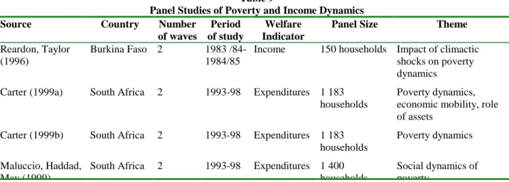
As underlined by Baulch and Hoddinott (2000:2), there are very few studies on individual poverty dynamics in developing countries, although developments in this field of research have recently begun (Table 9). Most of the work on the inter-temporal aspects of poverty has been conducted within a static comparative perspective. However, Chaudhuri and Ravallion (1994) demonstrated that static poverty indicators only distinguish quite inadequately the chronic poor from the transient poor. As mentioned in the introduction, the main cause for this shortcoming is the absence of longitudinal household surveys in most developing countries.
Table 9 lists the different studies conducted on poverty dynamics in developing countries. Half of them examine a few hundred households, and about 40% include only two points in time. The limited data available weakens the robustness of their results (limited sample representativeness, difficult identification of forms of the poverty, whether chronic and transient, and of the shocks experienced by the households).
These studies are different not only with respect to the length of time analyzed (and number of waves), but also to the geographic coverage. They also present a great diversity of methodological options and issues addressed. An important point is how to define chronic poverty and transient poverty, as two types of approaches co-exist. The first approach, the most common and the one we have adopted is based on crossings the poverty line, in a direction or another, which allows the definition of poverty states. Instead of distinguishing individuals or households in chronic or transient poverty, the second approach aims at isolating a chronic component and a transient component of income4. This approach was first used by Jalan and Ravallion (1998, 2000) in their study on rural households in Southern China, and then, for example, by McCulloch and Baulch (1998, 1999) in Pakistan. As pointed out by Yaqub, these two ways of defining poverty, as chronic or transient, are not equivalent. In this sense, in the case of a study on India by Gaiha and Deolikar (1993), among households whose permanent income was below the poverty line, only a third had current incomes below that line for each of the 9 periods covered by the survey (Yaqub, 2000:4). In the end, the extreme heterogeneity of the data and methods makes it difficult to compare results, identify patterns and, therefore, formulate policy proposals, differentiated according to the chronic or transient nature of the poverty encountered.
Table 9
Panel Studies of Poverty and Income Dynamics
Source Country Number
of waves
Period of study
Welfare Indicator
Panel Size Theme Reardon, Taylor
(1996)
Burkina Faso 2 1983 /84- 1984/85
Income 150 households Impact of climactic shocks on poverty dynamics
Carter (1999a) South Africa 2 1993-98 Expenditures 1 183 households
Poverty dynamics, economic mobility, role of assets
Carter (1999b) South Africa 2 1993-98 Expenditures 1 183 households
Poverty dynamics
Maluccio, Haddad, May (1999)
South Africa 2 1993-98 Expenditures 1 400 households
Social dynamics of poverty
4
Chronic poverty is defined as the gap between the poverty line and the average income over the entire period observed, while transient poverty is the remainder of total poverty minus chronic poverty.
May (1999) households poverty Dearcon, Krishnan
(2000)
Ethiopia 3 1994-95 Expenditures 1 450 households
Poverty dynamics and nutrition Gaiha (1989) India 3 1968/69-1970/71 Income 4 118 households Characteristics of the chronic poor Gaiha (1988) India 3 1968/69-1970/71 Income 4 118 households
Poverty transitions and economic mobility Gaiha, Deolalikar
(1993)
India 9 1975/76-1983/84
Income 170 households Chronic poverty according to different approaches Chaudhri, Ravallion (1994) India 8 1975/76-1982/83 Income, expenditures
170 households Methodological aspects in targeting policies aimed at the chronic poor Lanjouw, Stern
(1991)
India 4 1957/58- 1983/84
Income 143 households Poverty transitions
Walker, Ryan (1990)
India 10
1975/76-1984-85
Expenditures 240 households Socioeconomic dynamics
Grootaert, Kanbur (1995)
Ivory Coast 2 1985-86 Expenditures 700 households Poverty transitions
Grootaert, Kanbur, Oh (1997)
Ivory Coast 2 1987-88 Expenditures 700 households Factors determining per capita spending variations Herrera (1999) Peru 4 1985, 1990, 1994, 1996
Expenditures 460 households Factors determining poverty transitions, economic mobility
Herrera (2000a) Peru 3 1997-
1999 Expenditures 3 100 households Factors determining poverty transitions Cumpa, Webb (1999) Peru 3 1991, 1994, 1996
Expenditures 676 households Poverty transitions
Glewwe, Hall (1995)
Peru 2
1985/86-1990
Expenditures 699 households Factors determining per capita spending variations Jalan, Ravallion (1998) China 6 1985-90 Expenditures 38 000 individuals
Transient and chronic poverty and targeting the poor Jalan, Ravallion (2000) China 6 1985-90 Expenditures 38 000 individuals Factors determining transient and chronic poverty McCulloch, Calandrino (2002) China 5 1991-95 Income 3 311 households Poverty dynamics, vulnerability McCulloch, Baulch (1998) Pakistan 1986/87- 1990/91
Income 686 households Poverty transitions
McCulloch, Baulch (1999)
Pakistan 5 1986/87-
1990/91
Income 686 households Factors determining transient and chronic poverty
Mroz, Popkin (1995)
Russia 4 1992-94 Income 6 300 housing units
Poverty and employment transitions
Scott, Litchfield (1994)
Chile 2 1967/69-1985/86
Income 146 households Factors determining economic mobility and inequality
Scott (2000) Chile 2 1967/69-1985/86
Income 146 households Poverty transitions
Glewwe, Gragnolati, Zaman (2000) Vietnam 2 1992-93, 1997-98 Expenditures 4 281 households Factors determining transient and chronic poverty
Freire, S. (2000) Venezuela 2 1997-98 Income 7 744 households
Economic mobility and poverty transitions Sources: prepared by authors from Yaqub (2000a), Baulch, Hoddinott (2000: 7).
To our knowledge, the approach proposed here is the first comparative study on the factors that determine poverty transitions in two developing countries. To ensure result comparability, the data were treated strictly in the same manner: construction of the welfare indicator, definition of the poverty line, types of households, equal numbers of panel waves, study periods, estimation model and method and, lastly, independent variables. Regarding the latter, our study is distinct form the others, as it considered, besides the usual individual socioeconomic features of household heads and of the households to which they belong, the non-current shocks suffered by these households (labor market shocks, demographic shocks)5. Finally, this study is different from the ones presented above because of the fact that it took into account variables linked to the spatial location of households.
The Econometric Model
In the previous section on poverty transition profiles, we examined the unconditional risk that households with given characteristics may experience any of the poverty transition states. Through this, variables potentially relevant to policies to fight chronic and transient poverty were identified. A more analytical approach, however, requires that the specific effect of each variable be isolated, while maintaining the impact of the other variables constant. The present section will focus on modeling the factors associated with entries into and exits from poverty, as well as the conditions of « chronic poor » and « never poor. »
We chose to model poverty transitions rather than income dynamics.6 Our attention is therefore focused on discrete income variations on both sides of the poverty line. The dependent variable corresponds to the four states of poverty transition (chronic poverty7, exits from poverty, entries into poverty and non-poverty) observed from 1998 to 1999. The type of estimated model is multinomial logit, so the same variable may have a differentiated impact according to the type of poverty transition:
Pij (yi = 1 | xi) = 1/
∑
=4 2 j eβ(j)Xi Pij (yi = m | xi) = eβ(j)Xi /∑
j=42 1+ eβ(j)Xi pour 4>m>1Where Pij is the probability that household i is in poverty transition state j
Four groups of variables were used: three of them had to do with structural features concerning household heads, households and their neighborhood, and the fourth corresponded to variables related to shocks experienced by households, divided in two subgroups: demographic and economic shocks. To avoid the simultaneity and endogeneity problems mentioned above, the structural variables are those from the beginning of the period (1998) and the shock variables are those of the prior period (1997-1998), by taking advantage of the three observation points in time available. Variables were introduced block after block, which enabled us to assess the robustness of our results. The choice of this type of modeling requires several comments.
First, the choice of four states, in particular the distinction between entry into and exit from poverty within transient poverty, is justified by two types of related reasons. From the economic point of view, factors that may throw a household into poverty are not necessarily the same which, in the opposite direction, may enable it to exit poverty. The consideration of the potential existence of poverty traps should be enough to explain such asymmetry. In such a case, the policies to be implemented would therefore be different. This hypothesis is confirmed statistically, since, in both countries, Wald tests rejected the hypothesis that different transition states could be combined; the variables chosen therefore properly differentiate the four poverty states analyzed.
5
Therefore avoiding the problem of simultaneous bias found in certain studies in which panels only include two time periods (see Glewwe et al. 2000 on that point).
6