HAL Id: tel-00558768
https://tel.archives-ouvertes.fr/tel-00558768
Submitted on 24 Jan 2011HAL is a multi-disciplinary open access archive for the deposit and dissemination of sci-entific research documents, whether they are pub-lished or not. The documents may come from teaching and research institutions in France or abroad, or from public or private research centers.
L’archive ouverte pluridisciplinaire HAL, est destinée au dépôt et à la diffusion de documents scientifiques de niveau recherche, publiés ou non, émanant des établissements d’enseignement et de recherche français ou étrangers, des laboratoires publics ou privés.
K0s K0s K0s decays with the BABAR experiment
Simon Sitt
To cite this version:
Simon Sitt. Time-dependent analysis and amplitude analysis of B0 ! K0s K0s K0s decays with the BABAR experiment. Physique [physics]. Université Pierre et Marie Curie - Paris VI, 2010. Français. �tel-00558768�
École doctorale 517 "Particules, Noyaux et Cosmos "
THÈSE
Spécialité: Physique des particules
Présentée par
SITT Simon
Pour obtenir le grade de Docteur de l’Université Paris VI
Time-dependent analysis and amplitude analysis of
B
0→ K
0sK
0sK
0sdecays with the
B
AB
ARexperiment
Soutenue le 29 Septembre 2010
Jury :
Rapporteurs:
Stéphane Monteil
Christian Weiser
Examinateurs:
Tim Gershon
Emi Kou
Reynald Pain (Président du jury)
Abstract
Two independent analyses of the decay channel B0 → K0
sK0sK0s have been performed on a
data sample of 468 millions of B¯B pairs recorded by the BABAR detector at the PEP-II B
factory at SLAC National Laboratory.
The first analysis is a phase-space-integrated time-dependent analysis to extract the CP
vio-lation parameters S and C from the two sub-modes B0 → 3K0
s(π+π−) and
B0 → 2K0
s(π+π−)K0s(π0π0) simultaneously and to compare them to the charmonium
mea-surements. The result is
• S = −0.94+0.24−0.21± 0.06
• C = −0.17+0.18
−0.18± 0.04 ,
where the first uncertainty is statistical and the second is systematical. The result is com-patible within uncertainties with the Standard Model prediction and the charmonium modes measurements.
The second analysis is a time-integrated amplitude (or Dalitz plot) analysis to extract the in-clusive branching fraction and the branching fractions of the resonant modes that contribute to the decay. The result of the first amplitude analysis of this decay channel is
• B(B0 → K0 sK0sK0s) = (6.18 ± 0.47 ± 0.14 ± 0.06) × 10−6 • B(B0 → f 0(980)K0s; f0(980) → Ks0K0s) = (2.69+1.25−1.18± 0.35 ± 1.87) × 10−6 • B(B0 → f 0(1710)K0s; f0(1710) → Ks0K0s) = (0.50+0.46−0.23± 0.04 ± 0.12) × 10−6 • B(B0 → f 2(2010)K0s; f2(2010) → Ks0K0s) = (0.54+0.21−0.20± 0.03 ± 0.44) × 10−6 • B(B0 → Nonresonant; K0 sK0sK0s) = (13.31+2.23−2.30± 0.55 ± 2.77) × 10−6 • B(B0 → χ c0K0s; χc0→ K0sK0s) = (0.46+0.25−0.16± 0.01 ± 0.19) × 10−6,
where the first uncertainty is statististal, the second is systematical and the third corresponds
to Dalitz plot model uncertainties. No significant contribution of the controversial fX(1500)
resonance has been found. dummy
dummy dummy dummy dummy
Key words:
BaBar B mesontime-dependent CP asymmetry penguin
Dalitz plot analysis K meson
Branching ratio B0 → K0
Abstract
Deux analyses indépendantes du canal de désintegration B0 → K0
sK0sK0s ont été effectuées,
utilisant un échantillon de 468 millions de paires B¯B enregistrées par le détecteur BABAR
auprès de l’usine à B PEP-II à SLAC National Laboratory.
La première analyse est dépendant du temps et integrée sur l’espace de phase. Son but est
d’extraire simultanément des deux sous-canaux B0 → 3K0
s(π+π−) et
B0 → 2K0
s(π+π−)K0s(π0π0), les paramètres S et C de violation de CP . Il est intéressant de
comparer les valeurs mesurées avec les mesures des modes charmonium. Le résultat obtenu est
• S = −0.94+0.24
−0.21± 0.06
• C = −0.17+0.18−0.18± 0.04 ,
où la première incertitude est statistique et la deuxième est systématique. Ce résultat est compatible avec la prédiction du modèle standard et les mesures des modes charmonium. La deuxième analyse est une analyse en amplitude (ou dans le plan de Dalitz). Elle est intégrée sur le temps. Son but est d’extraire le rapport de branchement total, ainsi que les rapports de branchement des modes résonnants partiels. C’est la première fois que cette analyse est effectuée pour le canal étudié. Le résultat est
• B(B0 → K0 sK0sK0s) = (6.18 ± 0.47 ± 0.14 ± 0.06) × 10−6 • B(B0 → f 0(980)K0s; f0(980) → Ks0K0s) = (2.69+1.25−1.18± 0.35 ± 1.87) × 10−6 • B(B0 → f 0(1710)K0s; f0(1710) → Ks0K0s) = (0.50+0.46−0.23± 0.04 ± 0.12) × 10−6 • B(B0 → f 2(2010)K0s; f2(2010) → Ks0K0s) = (0.54+0.21−0.20± 0.03 ± 0.44) × 10−6 • B(B0 → Nonresonant; K0 sK0sK0s) = (13.31+2.23−2.30± 0.55 ± 2.77) × 10−6 • B(B0 → χ c0K0s; χc0→ K0sK0s) = (0.46+0.25−0.16± 0.01 ± 0.19) × 10−6,
où la première incertitude est statistique, la deuxième est systématique et la troisième est liée au modèle de l’amplitude. Aucun signal statistiquement significatif de la résonance
controversée fX(1500) n’a été observé. dummy
dummy dummy dummy
Mots clés:
BaBar méson Basymmetrie de CP dépendante du temps penguin
analyse en amplitude méson K
Rapport d’embranchement B0 → K0
Résumé en français
Le contexte théorique
Le modèle standard (MS) décrit les interactions fondamentales en dehors de la gravitation, à savoir les interactions électro-faible et forte. La physique des saveurs joue un rôle par-ticulier, puisque la saveur est conservée dans l’interaction forte mais pas dans l’interaction faible. Des particules à saveur non nulle (étranges, charmées, belles ...) peuvent être pro-duites (par paires) par les interactions fortes ou électro-magnétiques, mais ne peuvent se dés-intégrer que par l’interaction faible. Dans le MS les quarks ne sont pas en même temps des états propres de masse et de saveur, et la matrice unitaire de Cabbibo-Kobayashi-Maskawa (CKM) décrit les couplages faibles dans la base des états propres de masse. La matrice CKM peut être décrite par quatre paramètres, dont trois paramètres réels et une phase. La phase permet d’accommoder la violation de CP dans le MS. Cette dernière a été observée pour la première fois en 1964 dans la désintégration des kaons neutres et pourrait partiellement expliquer l’asymétrie entre matière et antimatière dans l’Univers. Une fois mesurés ces qua-tre paramèqua-tres, la théorie devient prédictive et permet de comparer les résultats de mesures expérimentales indépendantes avec leur prédictions théoriques. Ceci permet de tester les hy-pothèses qui ont été admises en construisant le MS, par exemple l’existence d’ exactement 3 familles de particules. L’unitarité de la matrice CKM de traduit par 6 relations qui peuvent être interprétées géométriquement comme reliant les côtés de triangles. Un de ces triangles, dont les angles sont appelés α, β et γ, n’est pas plat et est appelé triangle d’unitarité. La
rai-son d’être des usines à B, dontBABARet Belle, est la mesure de ce triangle, et en particulier
de l’angle β par le biais de la violation de CP dans le secteur des mésons B neutres. Les
mé-sons neutres portant de la saveur (K0, D0, B0) peuvent se transformer en leur anti-particule
(K0, D0, ¯B0) par le biais de diagrammes en boîte. Dans le cas des mésons B neutres, certains
couplages aux vertex de ces diagrammes portent la phase β. En mesurant la violation de CP dépendant du temps on peut avoir accès a cette phase : on observe l’interférence entre des
B0 qui se désintègrent dans un état final propre de CP, f
CP, et des B0 qui oscillent d’abord
en ¯B0 et se désintègrent ensuite dans le même état final f
CP. Au cas où un seul diagramme
contribue à ces désintégrations, ce qui est le cas avec une bonne approximation dans la
dés-intégration B0 → J/ψ K0
s, le paramètre S correspond à −ηCPsin(2β), où ηCP est la valeur
propre de fCPpour l’opérateur CP .
Avec davantage de données, une approche permettant de tester le MS consiste à mesurer in-dépendamment les côtés et les angles du triangle d’unitarité dans des processus différents, et à vérifier que toutes ces observables sont compatibles avec un seul triangle. Une incompatibi-lité pourrait signer la manifestation d’une nouvelle physique (NP). Cette thèse s’inscrit dans le contexte de ces recherches en analysant un canal supprimé dans le MS et qui pourrait être sensible à une nouvelle physique, car l’amplitude de désintégration dominante passe par
dans le MS.
Le cadre de travail: L’expérience B
A
B
AR
Le travail de recherche exposé dans cette thèse a été réalisé dans le cadre de l’expérience
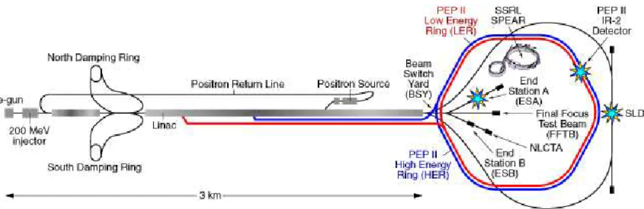
BABAR, collaboration internationale regroupant des institutions de dix pays. Le détecteur
BABAR est placé auprès du collisionneur PEP-II du SLAC National Laboratory, en
Cali-fornie (Etats-Unis). PEP-II est une usine à B, constituée d’un double anneau de stockage d’électrons et positrons. Les énergies des faisceaux sont ajustés à la résonance Υ (4S), dont
la masse est très légèrement supérieure au seuil de production des paires B¯B ; des mésons B
sont ainsi produits à un taux très élevé. La production dans un état cohérent et le fait que le
Υ (4S) est boosté dans le système du laboratoire, permettent la réalisation de mesures
dépen-dant du temps en étiquetant la saveur des mésons B. Le détecteurBABARa été conçu pour
enregistrer les produits des désintégrations des mésons B avec d’excellentes performances
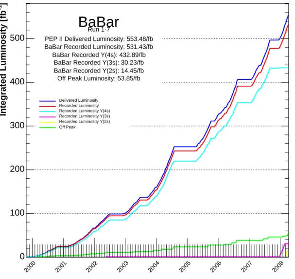
en termes d’efficacité et de résolution. La période de prise de données de l’expérienceBABAR
a commencé en 1999, s’est prolongée jusqu’en 2008 et a permis d’enregistrer 465 millions
de paires B¯B. La richesse et la qualité de la production scientifique de la collaboration
BABARcontribuent grandement aux succès actuels de la physique des saveurs. Cette thèse
comprend d’une part deux analyses de physique complémentaires du canal de
désintégra-tion B0 → K0
sK0sK0s et rend compte de deux études concernent la performance du détecteur
BABAR. Il s’agit d’une part d’une étude des effects de l’irradiation du détecteur de traces
en silicium (SVT), qui utilise des mesures de bruit en fonction de la tension de dépletion pour en déduire la dose absorbée, et d’autre part d’une étude de la différence entre
simula-tion et données dans la reconstrucsimula-tion dee π0, qui utilise des données et des désintegrations
D0 → K±π±π0 et D0 → K±π± simulées. Les deux analyses de physique sont détaillés
ci-dessous.
Analyses de physique
Aspects théoriques et expérimentaux du mode B
0→K
s0K
s0K
s0L’angle β a été mesuré avec une haute précision par les expériences BABAR et Belle dans
les modes B → c¯cK(∗) qui sont insensibles à des contributions possibles d’une nouvelle
physique. L’intérêt de l’analyse dépendant du temps est de comparer cette valeur a celle
obtenu dans le canal B0 → K0
sK0sK0s qui est supprimé dans le MS et qui procède par un
diagramme en boucle, dit "pingouin". Cette boucle pourrait inclure des contributions de particules virtuelles venant d’une "nouvelle physique", qui, par un couplage avec une phase différente, pourraient modifier la valeur de β. Comme l’état final est état propre de CP , il est possible d’extraire les paramètres S et C sans prendre en compte les résonances
intermédi-aires dans K0K0. Cependant il n’y a a priori aucune raison d’avoir les mêmes S et C pour tous
les états intermédiaires, qui son aussi états propres de CP (par exemple f0(980)K0s). Dans
La façon d’extraire le plus d’information possible des données, consite à faire deux analyses complémentaires : une analyse dépendant du temps mais intégrée sur le plan de Dalitz afin d’extraire les paramètres S et C inclusifs, et une deuxième analyse en amplitude intégrée sur le temps qui nous indique pour quelles contributions on a moyenné dans l’analyse dépendant du temps. Un autre aspect de l’analyse en amplitude est qu’elle peut contribuer à élucider le
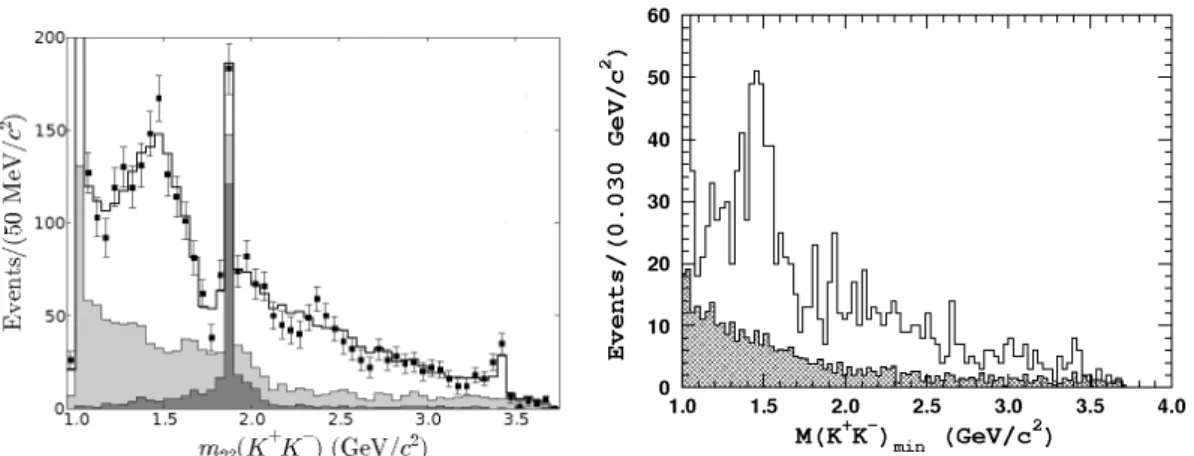
statut de la résonance controversée fX(1500) qui a été observée parBABARet Belle dans les
canaux B0 → K+K−K0
s et B+→ K+K−K+: du fait de la conservation du moment
ciné-tique, il ne peut y avoir que des résonances intermédiaires de spin pair. En conséquence, une
observation de cette résonance dans B0 → K0
sK0sK0s serait en faveur d’une résonance scalaire
et une non-observation en faveur d’une résonance vectorielle, comme cela a été suggéré par l’observation d’une résonance vectorielle par BES.
Un point particulier de ce canal avantageux pour l’analyse, mais nécessitant l’utilisation de techniques non-standard, est la présence de trois bosons identiques dans l’état final im-posant la symétrisation de l’amplitude. Cela mène à un plan de Dalitz avec une densité d’évènements six fois plus élevée que dans le cas de trois particules différentes. Il en ré-sulte une beaucoup plus grande sensibilité aux interférences entre résonances et malgré la statistique très limitée l’analyse reste faisable.
Analyse dépendant du temps du canal B
0→ K
0sK
0sK
0sL’analyse utilise un ajustement de vraisemblance généralisé. La fonction de vraisemblance contient une description du temps propre ∆t qui dépend de la saveur d’étiquetage et qui est fonction de S et C, et des variables qui servent à mieux séparer statistiquement signal et bruits de fond. Une sélection préalable permet d’enrichir les données en signal. De plus la
masse invariante de la résonance χc0 est exclue afin d’éviter une contribution charmée. Le
point crucial de l’analyse est la reconstruction précise du vertex de désintégration du B côté
signal afin de mesurer ∆t. Comme les K0
s ont un temps de vie non-négligeable et sont
neu-tres, ce vertex est reconstruit de façon indirecte en à l’aide d’un ajustement global des trois
K0
s en utilisant des contraintes géométriques. Pour assurer une bonne qualité d’ ajustement,
nous demandons qu’au moins un de ces K0
s soit de bonne qualité, evaluée par le nombre
d’impacts des pions chargés provenant de sa désintégration dans le détecteur de vertex. Nous
analysons les deux modes B0 → 3K0
s(π+π−) et B0 → 2K0s(π+π−)K0s(π0π0) simultanément
pour extraire les paramètres communs S et C. L’analyse est réalisée en aveugle, ce qui veut dire que l’outil d’analyse est complètement validé en utilisant des données simulées avant
de d’y passer les données. L’analyse de 3261 candidats dans le canal B0 → 3K0
s(π+π−) et
de 7209 candidats dans le canal B0 → 2K0
s(π+π−)K0s(π0π0) permet de trouver
respective-ment 201+16
−15évènements et 62+14−13évènements de signal. Les paramètres de violation de CP
trouvés dans les données sont
S = −0.935+0.238−0.214± 0.06 ,
C = −0.166+0.180
−0.178± 0.03
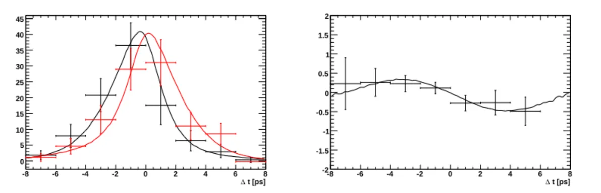
t [ps] ∆ -8 -6 -4 -2 0 2 4 6 8 0 5 10 15 20 25 30 35 t [ps] ∆ -8 -6 -4 -2 0 2 4 6 8 -2 -1.5 -1 -0.5 0 0.5 1
Figure 0.1:sPlots pour ∆t côté signal. A gauche sont montrées les distributions du temps
propre ∆t pour des mésons B côté signal (étiquetés comme B0 en noir et des
mésons B étiqueté comme ¯B0 en rouge). La figure de droite montre l’asymétrie
dépendant du temps.
correspond à l’incertitude systématique et inclut des incertitudes dûes à la statistique limitée des données simulées, aux différences entre simulations et données, au biais de l’ajustement, à l’incertitude des paramètres de violation de CP des bruits de fond et au veto utilisé pour rejeter les contributions de charmonium. L’incertitude dominante qui est due au vertexing sans traces directes venant du vertex de désintégration du méson B, est évaluée en estimant
les différences entre simulation et données dans un échantillon de contrôle B0 → J/ψ K0
s.
Analyse en amplitude du canal B
0→ K
0 sK
0sK
0sAfin d’étudier le contenu résonant, nous réalisons une analyse en amplitude du canal B0 →
K0
sK0sK0s en utilisant le modèle isobar pour extraire les modules et phases des amplitudes qui
contribuent. Contrairement à l’analyse dépendant du temps, on n’utilise que des événements
B0 → 3K0
s(π+π−) afin de réduire les bruits de fond et les événements de signal qui ne sont
pas correctement reconstruits. Comme mentionné plus haut, l’amplitude est symétrisée, ce qui est réalisé en construisant le plan de Dalitz avec les variables non ambigües de la masse
minimale smin et la masse maximale smax. Comme c’est la première analyse en amplitude
de ce canal, les contributions résonantes ne sont pas connues. Pour trouver un modèle du signal qui prend en compte toutes les contributions statistiquement significatives, on com-mence par un modèle de base qui inclut toutes les contributions de spin pair trouvées dans
l’analyse BABAR de B0 → K+K−K0s, sauf le fX(1500) controversé: f0(980), χc0 et
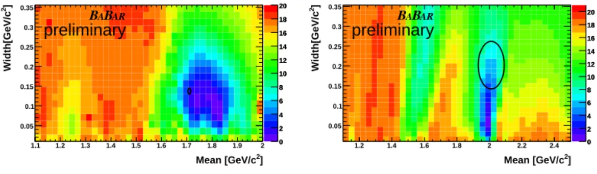
contri-bution non résonante. On utilise ensuite une méthode de vraisemblance dans laquelle on balaye l’espace bidimensionel des paramètres (masse et largeur) d’une résonance supplé-mentaire. On cherche des régions de vraisemblance accrue qui correspondent à la masse et à la largeur de résonances connues. On applique d’abord cette méthode pour une
réso-nance scalaire supplémentaire et on trouve une contribution de la f0(1710), illustré par la
Fig. 0.2. Aucune contribution de fX(1500) n’est visible. Ensuite f0(1710) est ajoutée au
modèle et on répéte la procédure pour une éventuelle résonance tensorielle. On trouve une
main-0 2 4 6 8 10 12 14 ] 2 Mean [GeV/c 1.1 1.2 1.3 1.4 1.5 1.6 1.7 1.8 1.9 2 Width[GeV/c 0.05 0.1 0.15 0.2 0.25 0 2 4 6 8 10 12 14 0 2 4 6 8 10 12 14 16 ] 2 Mean [GeV/c 1.2 1.4 1.6 1.8 2 2.2 2.4 Width[GeV/c 0.05 0.1 0.15 0.2 0.25 0 2 4 6 8 10 12 14 16
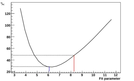
Figure 0.2: Vraisemblance traduite en χ2(−2∆logL) en fonction de la masse et de la largeur
d’une résonance scalaire additionnelle (à gauche) et d’une résonance tensorielle (à droite). Des régions de vraisemblance accrue correspondent à des petites valeurs de −2∆logL (le maximum correspond à −2∆logL = 0). Les ellipses
indiquent les valeurs mesurées des résonances f0(980) et f2(2010) issus de la
Ref. [1].
tenant f0(980), χc0, f0(1710), f2(2010) et une contribution non résonante nous effectuons
l’ajustement final aux données. L’utilisation de la vraisemblance généralisé avec 505
can-didats fournit 200 ± 15 événements de signal B0 → K0
sK0sK0s et 305 ± 18 événements de
bruit de fond (les incertitudes sont statistiques seulement). Les projections du résultat de l’ajustement sur les axes du plan de Dalitz sont montrées sur la Fig. 0.3. Nous traduisons les
] 2 [GeV/c min s 1 1.2 1.4 1.6 1.8 2 2.2 2.4 2.6 2.8 3 3.2 -4-2 0 2 4 0 10 20 30 40 50 60 70 80 BABAR preliminary ] 2 [GeV/c max s 3.2 3.4 3.6 3.8 4 4.2 4.4 4.6 -4-2 0 2 4 0 10 20 30 40 50 60 70 BABAR preliminary
Figure 0.3: Projections du résultat de l’ajustement sur les axes du plan de Dalitz( smin à
gauche et smax à droite). Les données sont indiquées avec leurs barres d’erreur.
La ligne rouge tireté (pointillée bleue) correspond au signal (bruit de fond) et la ligne noire correspond au modèle total.
magnitudes et phases des contributions au modèle en fractions isobares (FF), les valeurs étant résumées dans le Tab. 0.1. I existe une deuxième solution à l’ajustement, différant de celle qui correspond au maximum par presque deux écart-types. Les valeurs correspondantes sont également montrées. En utilisant les fractions et le rapport de branchement inclusif obtenu par le nombre d’évènements signal nous calculons les rapports de branchement individu-els. Les valeurs obtenues pour la meilleure solution sont montrées dans le Tab. 0.2. Les
seulement. La signification statistique a été évaluée par la variation de la
vraisem-blance quand la contribution est retiré du modèle (Significance = √−2∆logL).
Tous les modes résonants ont une signification statistique de moins de 5 écart-types.
Mode Solution 1 Solution 2
FF f0(980)K0s 0.44+0.20−0.19 1.03+0.22−0.17 Phase [rad]f0(980)K0s 0.09 ± 0.16 1.26 ± 0.17 Significance [σ]f0(980)K0s 3.3 -FF f0(1710)K0s 0.07+0.07−0.03 0.09+0.05−0.02 Phase [rad] f0(1710)K0s 1.11 ± 0.23 0.36 ± 0.20 Significance [σ]f0(1710)K0s 3.7 -FF f2(2010)K0s 0.09+0.03−0.03 0.10 ± 0.02 Phase [rad] f2(2010)K0s 2.50 ±0.20 1.58 ± 0.22 Significance [σ]f2(2010)Ks0 3.3 -FFχc0K0s 0.07+0.04−0.02 0.07 ± 0.02 Phase [rad]χc0K0s 0.63 ± 0.47 -0.24 ± 0.52 Significance [σ]χc0Ks0 4.2 -FF NR 2.15+0.36 −0.37 1.37+0.26−0.21 Phase [rad] NR 0.0 0.0 Significance [σ]NR 8.2 -Total FF 2.84+0.71−0.66 2.66+0.35−0.27
en multipliant les fractions isobars correspondantes, obtenus dans la meilleure
solution, avec le rapport de branchement inclusif de B0 → K0
sK0sK0s. La première
incertitude est statistique, la deuxième est systématique et la troisième correspond aux incertitudes liées au modèle du plan de Dalitz.
Mode B(B0 → Mode)[10−6] Inclusive B(B0 → K0 sK0sK0s) 6.186 ± 0.475 ± 0.145 ± 0.067 f0(980)K0s, f0(980) → K0sK0s 2.696+1.250−1.188± 0.357 ± 1.874 f0(1710)K0s, f0(1710) → K0sK0s 0.502+0.461−0.235± 0.043 ± 0.129 f2(2010)K0s, f2(2010) → K0sK0s 0.543+0.214−0.204± 0.034 ± 0.440 NR, K0 sK0sK0s 13.315+2.234−2.302± 0.554 ± 2.779 χc0K0s, χc0 → K0sK0s 0.462+0.252−0.165± 0.015 ± 0.197
incertitudes systématiques comprennent des incertitudes liées aux paramètres de la fonction de vraisemblance, à l’efficacité de reconstruction, aux bruits de fonds négligés, au biais de
l’ajustement et au nombre de paires de B¯B produits dans PEP-II . Les incertitudes liées au
modèle de l’amplitude sont dues aux erreurs sur les mesures des masses et des largeur des contributions résonantes et aux contributions résonantes statistiquement non-significatives qui n’ont pas été incluses dans le modèle. La plus grande incertitude dans le modèle est dûe
à la mesure peu précise de la f2(2010).
Discussion des résultats physiques
L’analyse dépendant du temps a permis de trouver des paramètres S et C qui sont compatibles à un écart-type avec la prédiction du MS. L’analyse en amplitude a permis de mesurer pour
la première fois les modes résonants contribuant à la désintégration B0 → K0
sK0sK0s et trouve
des contributions de f0(980), χc0, f0(1710), f2(2010) et une contribution non resonante. Les
deux analyses sont statistiquement très limitées : dans l’analyse dépendante du temps cela
se traduit par le fait que la limite du domaine physique (S2 + C2 ≤ 1), est à moins d’un
écart-type de l’incertitude. Dans l’analyse en amplitude, aucune contribution résonante n’a une signification statistique supérieur a 5 écart-types.
I thank Stéphane Monteil and Christian Weiser for having accepted to be referees and Tim Gershon, Emi Kou and Reynald Pain for having accepted to be members of the jury for my thesis.
I am grateful to Pacal Debu and Reynald Pain for hosting me at the LPNHE during my thesis. I want to especially thank my supervisor Eli, who was always available, for exceptional three years, for the very friendly and efficient working atmosphere (even when deadlines are close) and for all he taught me.
A special thanks goes to my collaborator at SLAC, Matt Graham, for his help, his very effi-cient way of doing things and for the great atmosphere we had in our small analysis group.
I would also like to thank:
The BABAR group at LPNHE: Jacques Chauveau, Eli Ben-Haim, José Ocariz, Alejandro
Perez, Jennifer Prendki, Pablo del Amo Sanchez, Giovanni Calderini and Giovanni Mar-chiori. Jacques who was always there for advice and willing to do the final reading of this document. José for the many interesting discussions and his inputs. Alejandro for his help and the great time we spent together at SLAC and elsewhere. Pablo for his help, in particular
for the π0efficiency study, the many physics and non-physics discussions over lunch and his
inputs to the analyses. Giovanni C., with whom I did the SVT radiation damage study, for giving me the chance to do a hardware-related study.
The whole BABAR collaboration, in particular the Charmless 3-Body B Decays Analysis
Working Group, and Tim Gershon, Tom Latham and Enrico Robutti for their attention and valuable comments during the internal review of the analyses.
The theorists and experimentalist who helped us when we got confused with quantum me-chanics: Sébastien Descôtes-Genon, Emi Kou, Patrick Roudeau, Alain Le Yaouanc and Zoltan Ligeti.
Achille Stocchi for his inputs to the SuperB study.
The whole staff of the LPNHE, in particular fellow graduate students and my "parrain" Jean-Michel.
Contents
I
Introduction
21
1.1 CP violation . . . . 23
1.2 Flavor physics and charmless-3-body B decays . . . 24
1.3 Overview . . . 24
II
Theoretical and experimental context
27
2 Quark mixing and CP violation 29 2.1 Quark Mixing and CKM matrix . . . 292.2 CP violation in the B meson system . . . 31
2.2.1 Introduction . . . 31
2.2.2 The neutral B system, mixing and time dependent CP asymmetry . 32 2.2.3 Different types of CP violation in the B mesons system . . . . 33
2.2.4 Experimental status of the CKM parameters . . . 36
3 Charmless 3-body B decays and B0→K0 sKs0Ks0 39 3.1 Search for new Physics in b →s Penguin dominated modes . . . . 39
3.2 Particularities of the decay B0→K0 sKs0Ks0 . . . 40
3.2.1 Theoretical predictions for TDCPV parameters of the decay B0→K0 sKs0Ks0 42 3.2.2 Restrictions on the final state due to angular momentum conservation 43 3.2.3 The controversial fX(1500) resonance . . . 44
3.3 3-body decays . . . 45
3.3.1 Kinematics and Dalitz plot formalism . . . 45
3.3.2 The isobar model . . . 47
3.3.3 Mass term description . . . 48
3.3.4 Barrier factors . . . 50
3.3.5 Angular distribution . . . 50
3.3.6 Symmetrized amplitude . . . 50
3.3.7 Square Dalitz plot (SDP) . . . 53
3.3.8 Observables . . . 55
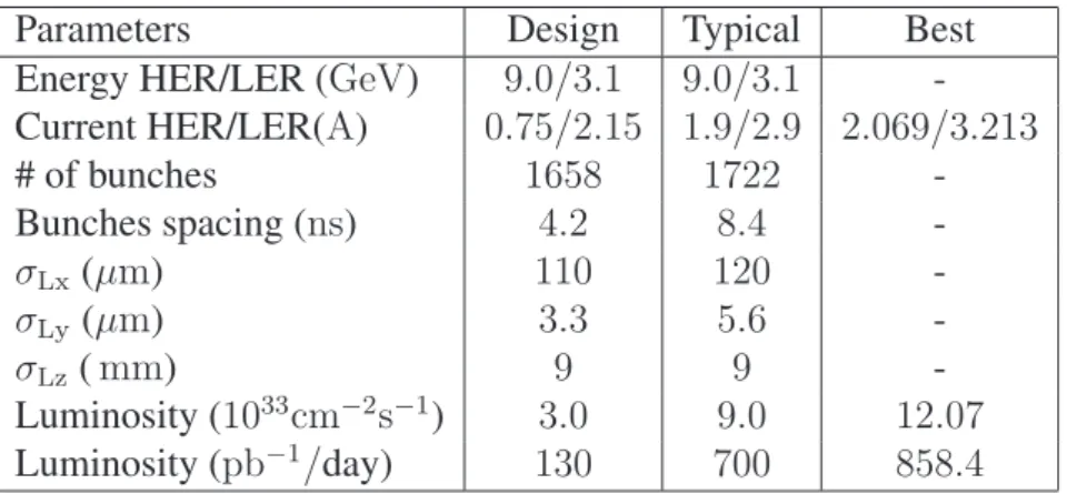
4 The PEP-II 2 B-Factory and the BABARDetector 57 4.1 An asymmetric e+e−collider as a B factory . . . . 57
4.2 PEP-II and the B Factory . . . . 58
4.2.1 The Interaction Region . . . 59
4.2.2 Machine backgrounds . . . 60
4.2.3 Trickle injection . . . 60
4.2.4 Performance . . . 61
4.3 TheBABARdetector . . . 62
4.4 Silicon Vertex Tracker . . . 63
4.4.1 Physics requirements . . . 63 4.4.2 Design . . . 63 4.4.3 Performance . . . 65 4.5 Drift Chamber . . . 65 4.5.1 Physics requirements . . . 65 4.5.2 Design . . . 67 4.5.3 Performance . . . 68
4.6 Detector of Internally Reflected Cerencov light . . . . 69
4.6.1 Physics requirements . . . 69 4.6.2 Design . . . 69 4.6.3 Performance . . . 70 4.7 Electromagnetic Calorimeter . . . 71 4.7.1 Physics requirements . . . 71 4.7.2 Design . . . 71 4.7.3 Performance . . . 72
4.8 Instrumented Flux Return . . . 72
4.8.1 Physics requirements . . . 72
4.8.2 Design . . . 73
4.8.3 Performance . . . 75
4.8.4 Limited streamer tubes . . . 75
4.9 Trigger . . . 75
4.9.1 Level-1 trigger . . . 76
4.9.2 Level-3 trigger . . . 76
4.10 Data Aqcuisition . . . 77
4.11 Online Prompt Reconstruction . . . 77
5 Radiation damage study of the SVT 79 5.1 Introduction . . . 79
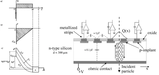
5.2 Theoretical aspects of radiation damage in silicon detectors . . . 79
5.2.1 Selection of basic features of silicon detectors . . . 79
5.2.2 Damage mechanism . . . 82
5.3 Measurement and analysis . . . 85
5.3.1 Overview and analysis strategy . . . 85
5.3.2 Extraction of Vdepfrom noise measurements . . . 86
5.3.3 Data analysis . . . 87
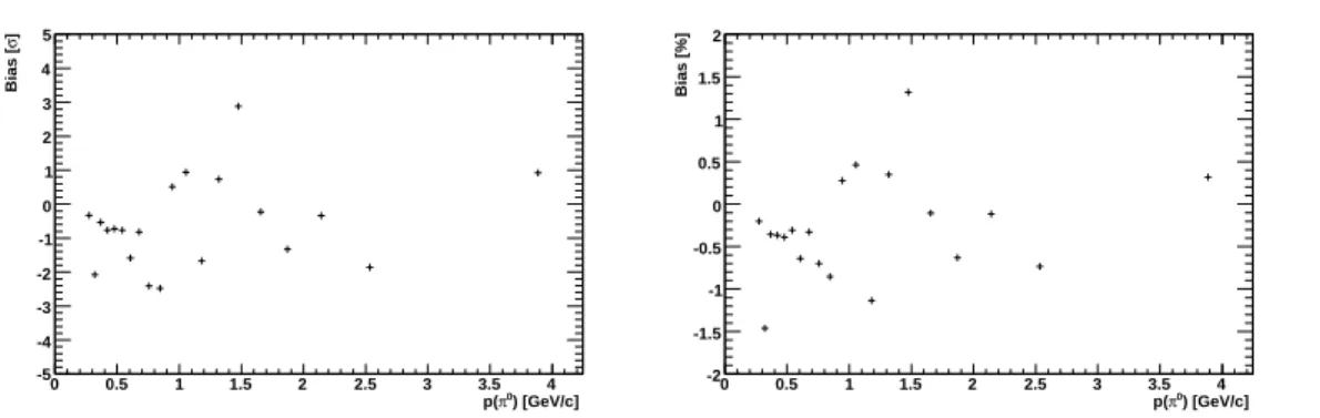
6 Study of the π0 reconstruction efficiency 93
6.1 Introduction . . . 93
6.1.1 Motivation for the study . . . 93
6.1.2 Analysis strategy . . . 94
6.2 Reconstruction . . . 95
6.2.1 Data samples . . . 95
6.2.2 Reconstruction . . . 95
6.3 Selection and backgrounds . . . 96
6.3.1 Selection for D0 → Kπ . . . . 96
6.3.2 Additional selection for D0 → Kππ0 . . . . 96
6.3.3 Candidate selection . . . 97
6.3.4 Signal and background categories . . . 98
6.4 The likelihood fits . . . 101
6.5 Fit validation . . . 105
6.6 Systematic uncertainties . . . 106
6.7 Results . . . 106
III Analysis of B
0→K
0 sK
s0K
s0111
7 Reconstruction and analysis techniques 113 7.1 Introduction . . . 1137.2 Data Samples . . . 113
7.2.1 On-peak and off-peak data samples . . . 113
7.2.2 Simulation (Monte Carlo) data samples . . . 114
7.3 Reconstruction . . . 116
7.3.1 Tracking . . . 116
7.3.2 Calorimeter algorithms . . . 117
7.3.3 Particle identification (PID) . . . 118
7.3.4 Flavor tagging . . . 118
7.3.5 Vertexing . . . 121
7.4 The ∆t measurement . . . 122
7.4.1 The ∆z measurement . . . 122
7.4.2 The ∆t determination . . . 123
7.4.3 The ∆t resolution model . . . 124
7.5 Discriminating variables . . . 124
7.5.1 B meson kinematic variables . . . 124
7.5.2 K0 s kinematic variables . . . 125
7.5.3 Event-shape variables and Neural Network (NN) . . . 125
7.6 Maximum likelihood fits . . . 129
7.6.1 General aspects of likelihood fitting . . . 129
7.6.2 The likelihood scan technique . . . 130
8 Time Dependent B0 → K0
sK0sK0s Analysis 133
8.1 Introduction . . . 133
8.2 Selection and backgrounds . . . 133
8.2.1 Common selection criteria in the two submodes . . . 133
8.2.2 Event selection for the B0 → 3K0 s(π+π+) submode . . . 134
8.2.3 Event selection for the B0 → 2K0 s(π+π−)Ks0(π0π0) submode . . . 135
8.2.4 Vertex requirements . . . 138
8.2.5 Continuum background . . . 138
8.2.6 Background from B Decays . . . . 140
8.2.7 Charmonium Vetoes . . . 142
8.3 Maximum likelihood fit . . . 144
8.3.1 Likelihood function . . . 144
8.3.2 The PDF . . . 145
8.4 Validation studies . . . 148
8.4.1 Fits to MC . . . 148
8.4.2 Pure toy studies . . . 151
8.4.3 Embedded toys . . . 152
8.5 Results . . . 153
8.6 Systematic uncertainties . . . 157
8.6.1 Statistical uncertainty of PDFs taken from simulation . . . 159
8.6.2 MC-data differences for PDFs taken from simulation . . . 160
8.6.3 Statistical uncertainty of PDFs taken from data . . . 162
8.6.4 Fit Bias . . . 162
8.6.5 Uncertainty in the B and CP content of the B-background . . . . . 162
8.6.6 Bias linked with the charmonium vetoes . . . 163
8.6.7 Miscellanea . . . 163
8.7 Summary . . . 163
9 Amplitude Analysis 165 9.1 Introduction . . . 165
9.2 Selection and backgrounds . . . 165
9.2.1 Selection and Selection Efficiencies . . . 165
9.2.2 Continuum background . . . 166
9.2.3 Background from B decays . . . 169
9.3 Maximum likelihood fit . . . 169
9.3.1 Likelihood function . . . 169
9.4 Determination of the signal model . . . 173
9.4.1 The "baseline" model . . . 173
9.4.2 Likelihood scans . . . 173
9.4.3 Variation of the likelihood as function of single events . . . 177
9.4.4 Add/remove . . . 177
9.5 Validation tests . . . 179
9.5.1 Validation of baseline model . . . 179
9.6 Results . . . 182
9.7 Systematic uncertainties . . . 187
9.7.1 PDF parameters and non-parametric PDFs of discriminating variables 187 9.7.2 B background . . . 190 9.7.3 Fit bias . . . 191 9.7.4 Reconstruction efficiency . . . 191 9.7.5 Model uncertainties . . . 192 9.7.6 Uncertainty on NBB. . . 193 9.8 Summary . . . 193
IV SuperB prospective of B
0→K
0 sK
s0K
s0195
10 Super B-factory prospective 197 10.1 Introduction . . . 19710.2 Error projection using theBABARsetup . . . 197
10.3 The SuperB experiment . . . 200
10.3.1 The SuperB factory . . . 200
10.3.2 The SuperB detector . . . 201
10.4 SuperB studies using FastSim . . . 203
10.4.1 What is FastSim? . . . 203
10.4.2 Efficiencies and beam backgrounds . . . 204
10.4.3 Vertex measurement . . . 206 10.5 Summary . . . 208
V Appendix
211
A π0 efficiency 213 B TD analysis 237 C DP analysis 247Part I
1.1 CP violation
When a particle and a antiparticle are created in pair from energy, it is intuitive to think that they behave and decay in the same way. Why wouldn’t they? They are exactly the same, except the quantum numbers have changed signs. The quantum mechanical operator that transforms a particle into its anti-particle is the charge conjugation C. It changes the sign of all internal quantum numbers (charge, baryon number, lepton number, strangeness, charm, beauty, truth) while leaving the mass, energy, momentum and spin untouched. While C is conserved in the strong and electromagnetic interaction, this is not the case for the weak interaction. For instance, if one applies C on a left-handed neutrino, as the spin is conserved in the transformation, the result is a left-handed anti-neutrino, but left-handed anti-neutrinos do not exist and C is therefore maximally violated.
An operation that turns a left-handed neutrino into a right-handed anti-neutrino does not only need to invert the internal quantum numbers, but also the spin of the particle. This is done by the parity operator P that does the transformation ~x → −~x, i.e. the spin is inverted. The combined operation of charge conjugation and parity (CP ) reproduces what we observe in nature: it turns left-handed particles into right-handed anti-particles. While C and P are maximally violated in the weak interaction, their combination was expected by most physicists to be an exact symmetry. This assumption has been proven wrong in 1964 when
Cronin, Fitch, Christenson and Turlay [2] showed experimentally that neutral K0
L mesons
do not always decay to CP eigenstates with a CP eigenvalue of -1 (three pions in the final state) as expected, but that a small fraction also decays to final states with CP eigenvalue of +1 (two pions).
If CP is not an exact symmetry of nature, particles and anti-particles can decay differently. This is why CP violation (CPV) is a candidate to explain cosmological observations that find no sign of free anti-matter, while the Big Bang theory assumes creation of an equal amount of matter and anti-matter out of energy [3].
In the standard model of particle physics (SM), CP violation can be accommodated by a non-zero weak phase in the Lagrangian (see Sec. 2.1). In the SM picture, CP violation is an interference effect that can be measurable when several amplitudes with different phases contribute to the transition amplitude of a decay (see Sec. 2.2.3). In the case of neutral flavored mesons, a second amplitude that can lead to interference is engendered by "mixing"
(see Sec. 2.2.2). In the case of the neutral B mesons, the oscillation frequency between B0
and it’s anti-particle ¯B0 is of the same order of magnitude as the lifetime of these particles.
As a result the interfering amplitudes are of comparable sizes which makes the B0B¯0system
a privileged laboratory for measuring CP violating effects. From an experimental point of
view, to measure a difference between the decays of B0 and ¯B0, one needs to identify the
flavor of the B meson under study, as both neutral B mesons have access to the same final state. The experimental setup in the B factories is optimized for this kind of measurement,
as the B0B¯0 system is produced in a coherent L=1 state through the decay of the Υ(4S)
resonance. In this coherent state, there is always exactly one B0 and one ¯B0. When one of
them, Btag, decays to a flavor specific state, the other one, BCP, has at the same moment
the opposite flavor. As neutral B mesons oscillate as a function of time, one also needs to
of ∆t (see Sec. 7.4) the B factories have been designed as asymmetric e+e− colliders. Her the Υ (4S) is boosted in the laboratory frame and the short-lived B mesons (∼1.5 ps) travel an average distance of 256 µm, which is measurable in the detector. As the boost in known,
∆t can be measured through the distance between the decay vertices of Btagand BCP.
1.2 Flavor physics and charmless-3-body B decays
The flavor sector of the SM is strongly constrained by the CKM formalism that describes flavor couplings. The unitarity of the CKM matrix implies relations between the matrix ele-ments that can be geometrically interpreted as unitarity triangles (UT). This means once two angles or sides of a UT are measured, the theory becomes predictive. CP violation in the B meson system is directly linked to the flavor coupling and gives access to UT properties (see Sec. 2.2.3). Together with other measurements [4] [5], the UT can be over constrained and used to test the SM (see Fig. 2.5). If the different measurements are not compatible with one single UT, this can be a sign of new physics (NP) contributions (see Sec. 3.1). Given that all current measurements agree with the SM, NP contributions are expected to be small. This is why the search of NP is most promising in processes where the SM contribution is small. b → s charmless-3-body B decays are good candidates for the search of NP, as they are suppressed in the SM and dominated by loop diagrams (penguin diagrams, see Sec. 3.1) that could have virtual contributions from NP particles.
B0 → K0
sK0sK0s is a privileged channel for the search of NP: not only it is experimentally
clean (see Sec. 7.3) but also it is impaired by small theoretical uncertainties (see Sec. 3.2.1). Additionally the final state is CP definite (see Sec. 3.2.2) and the CP violation parameters can be measured without an amplitude analysis. Independently, an amplitude analysis can
provide information on the mKK spectrum. In particular, the unclear nature for the
con-troversial fX(1500) resonance (see Sec. 3.2.3) can be constrained because only even-spin
resonances are permitted due to angular momentum conservation. An observation of this resonance would make a scalar nature more likely and in case of non-observation a vector nature would be favored. Our reconstruction method is common to both the time-dependent
CP violation analysis (TDCPV) and the amplitude analysis, and so are also most analysis
techniques (Chap. 7).
1.3 Overview
In part II we describe the theoretical and experimental context of this work. A general introduction to CP violation in the B meson system in the context of the SM is given in
Chap. 2, while more detailed information on charmless 3-body B decays with focus on B0 →
K0
sKs0Ks0 can be found in Chap. 3. In the following Chap. 4, the BABAR detector and the
PEP-II collider are presented. This part also includes detector-related studies: in Chap. 5 we present a radiation damage study oft the silicon vertex detector and in Chap. 6 a study of the
π0reconstruction efficiency.
Part III represents the core of this work, where the analysis techniques are presented in Chap. 7 while the time-dependent analysis is described in Chap. 8 and the amplitude analysis
is described in Chap. 9.
Part IV concludes this work with the prospectives of the time-dependent analysis in the context of the SuperB project.
Part II
2 Quark mixing and CP violation
2.1 Quark Mixing and CKM matrix
In the SM1, interactions between elementary particles are mediated by gauge bosons. These
gauge bosons are associated with the invariance of the Lagrangian under abelian and non-abelian gauge transformations [6].
The weak interaction is mediated by the W± and Z0 bosons that are generated by the
non-abelian SU(2) flavor group. The quark content of the SM are three left-handed flavor doublets and six right-handed flavor singlets. Each doublet consists of one up-type quark and one
down-type quark. µ u d ¶ µ c s ¶ µ t b ¶ . (2.1)
The part of the Lagrangian that describes flavor changing charged currents between quarks is LCC = −g 2 · ¡ ¯u ¯c ¯t¢LγµVCKM ds b L W+µ + h.c. , (2.2)
where (u,c,t) are the up-type left-handed quarks, (d,s,b) are the down-type left-handed quarks,
g is the SU(2)L coupling constant and Wµ is the W boson field operator. Flavor changing
neutral currents are not allowed in the SM and right-handed quarks are not subject to flavor changing transitions as they are singlets. By convention one works with mass eigenstates, but the couplings between quarks mix flavors, and the quark mass eigenstates are not the
quark flavor eigenstates. The matrix VCKM
VCKM= VVudcd VVuscs VVubcb Vtd Vts Vtb (2.3)
is the unitary matrix that describes quark mixing in the Cabbibo-Kobayashi-Maskawa
for-malism [7]. In other words VCKM gives the SU(2) flavor couplings in the basis where the
quark mass matrix is diagonal and real. The non-diagonal terms of the matrix allow flavor changing transitions between quarks, i.e. transitions between quarks from different flavor doublets.
A priori a 3x3 unitary complex matrix has 9 degrees of freedom, i.e. it can be parameterized with three angles and 6 phases. By redefining the phases of the quark fields, this parameter-ization can be reduced to three mixing angles and a single phase.
1This section is non-exhaustive, a detailed description of the Standard Model of particle physics (SM) can be found in [6]
With such a particular quark field phase convention, the mixing matrix can be written in the so-called "standard parameterization" [8]:
VCKM = c12c13 s12c13 s13e −iδ −s12c23− c12s23s13eiδ c12c23− s12s23s13eiδ s23c13 s12s23− c12c23s13eiδ −c12s23− s12c23s13eiδ c23c13 . (2.4)
This single phase δ allows the possibility of CP violation in the SM [7] but CP violation is not a necessary feature of the SM. There could be further "accidental" symmetries such as two quarks of the same charge could have the same mass, or the value of one of the angles could be zero or π/2 or the phase itself could be zero. In these scenarios, the number of parameters could be reduced even further and CP violation would no longer be possible. Experimental data shows that there is a hierarchy among the matrix elements and that the matrix is dominated by its diagonal terms. This means that transitions inside flavor doublets are preferred. An experimentally more convenient parameterization has been proposed by Wolfenstein [9]: VCKM = 1 − λ2 2 λ Aλ3(ρ − iη) −λ 1 −λ2 2 Aλ2
Aλ3(1 − ρ − iη) −Aλ2 1
+ O(λ4) , (2.5)
where the parameters A, λ, ρ and η are defined with respect to the standard parameterization as follows
s12 ≡ λ ,
s23 ≡ Aλ2,
s13e−iδ ≡ Aλ3(ρ − iη) ≡ Aλ
3
1−λ2/2(¯ρ − i¯η) .
(2.6) The advantage is that we know from experimental data that the λ parameter is small (λ '
|Vus| ' 0.22), and the Taylor development of the matrix elements that is shown in Eq. 2.5
is sufficiently accurate for most experimental and phenomenological considerations. The
unitarity of the CKM matrix (VV† = V†V = 1) implies 9 constraints among the matrix
elements, 3 that result from the normalization of the columns and 6 that result from the vanishing product of pairs of different columns and rows.
Three of them are of particular interest for the study of CP violation, as they are more sensitive to the non-reducible CKM phase:
VudV∗us+ VcdV∗cs+ VtdVts∗ = 0 , (2.7)
VusV∗ub+ VcsV∗cb+ VtsV∗tb = 0 , (2.8)
VudV∗ub+ VcdV∗cb+ VtdVtb∗ = 0 . (2.9)
A null sum of three complex numbers can be interpreted geometrically as a triangle in the complex plane. Equations 2.7, 2.8 and 2.9 are the basis of the so-called unitarity triangles. In
the following we concentrate on the third triangle as it is related to B0B¯0mixing (via V
tdV∗tb,
see 2.2.2), charmed semileptonic and charmless B decays. If we divide 2.9 by VcdVcb∗ we
get a convention-independent definition of the unitarity triangle (UT)
VudV∗ub
VcdV∗cb
+ 1 + VtdV∗tb
VcdV∗cb
Using 2.5 it can be shown that all sides of this triangle are of the same order of magnitude.
The vertices are exactly (0,0), (1,0) and (¯ρ,¯η), where ¯ρ + i¯η = −VudV∗ub
VcdV∗cb is phase definition
independent. The triangle is shown in Fig. 2.1.
Figure 2.1: Sketch of the unitarity triangle. The coordinates ¯ρ and ¯η are defined in Eq. 2.6
The angles α, β and γ are defined as
α ≡ arg ³ −VtdVtb∗ VudVub∗ ´ , β ≡ arg ³ −VcdV∗cb VtdV∗tb ´ , γ ≡ arg ³ −VudV∗ub VcdV∗cb ´ , (2.11)
The UT is of particular experimental and theoretical interest, as it can be over-constrained by independent measurements. There are three sides and three angles that can be measured, but a triangle is already well defined with three out of this six constraints. One of the main goals of the B factories is to make as many independent measurements as possible: If the SM is valid, all these independent measurements should be compatible with the same triangle, whereas if this is not the case, this is a sign of non-SM contributions to the decay amplitudes. We show the current experimental constraints of the UT in Sec. 2.2.4.
2.2 CP violation in the B meson system
2.2.1 Introduction
B mesons have the heaviest quark that forms bound states, the b quark, as valence quark. Studying decays of heavy flavored mesons, e.g. in semi-leptonic decays, can give yield in-formation of CKM elements [6]. Another way to measure CKM elements is through mixing induced phenomena. The neutral B mesons have a lifetime τ = 1.530 ± 0.009 ps that is of
the same order of magnitude as their oscillation period (T = 1
∆md =
1
0.51 ps−1 = 1.96ps).
2.2.2 The neutral B system, mixing and time dependent CP
asymmetry
Mixing in the neutral B system
The neutral B0meson and its CP conjugate the ¯B0meson are defined by their flavor contents
(¯bd) and (b¯d), respectively. While the B0 and ¯B0 mesons are produced via the strong and
electro-magnetic interactions, we know from their lifetime that the decay proceeds via the
weak interaction. Before its decay, the development in time of the physical B meson B0
phys
is governed by its effective Hamiltonian. As there are flavor-non-conserving weak processes
that connect the flavor eigenstates, the effective Hamiltonian is non-diagonal in the {B0, ¯B0}
base [10]: Heff = µ H0 H12 H21 H0 ¶ = M − i 2Γ = µ M0 M12 M∗ 21 M0 ¶ − i 2 µ Γ0 Γ12 Γ∗ 21 Γ0 ¶ (2.12) The assumption of CPT invariance constrains the diagonal terms of the matrices to be the same. The effective Hamiltonian is not Hermitian to take into account the decay of the particle. The real part describes oscillation between flavor eigenstates and the imaginary
part the decay. Feynman representations of weak transitions between B0and ¯B0are shown in
Fig. 2.2. It results that the mass eigenstates of the neutral B meson system are a superposition
d b W W t,c,u u , c , t d b d b t,c,u t,c,u W W d b
Figure 2.2: Box Feynman diagrams weakly mediated transitions between B0and ¯B0 flavour
eigenstates
of B0 and ¯B0 flavor eigenstates. They are called B
L(ight) and BH(eavy) with mass eigenvalues
MLand MHand width eigenvalues ΓL and ΓH.
|BL ® = p|B0®+q| ¯B0®, |B H ® = p|B0®−q| ¯B0®, (2.13)
where p and q are complex numbers that satisfy |p|2 + |q|2 = 1. The mass and width
differences are defined as follows:
∆md= MH− ML, ∆Γ = ΓH− ΓL, (2.14)
where ∆md is positive by definition and corresponds to the mixing frequency. The ratio of
the q and p parameters is given by q
p = −
∆md− 2i∆Γ
2(M12−2iΓ12)
All the information of the time development of the system is contained in the Hamiltonian,
i.e the oscillation of the physical B meson B0
physbetween flavor eigenstates through weak
in-teraction can be described by the eigenvalues of the Hamiltonian and the q and p parameters.
|B0 phys(t)i = g+(t)|B0i − q pg−(t)|¯B 0i (2.16) |¯B0phys(t)i = g+(t)|¯B0i − p qg−(t)|B 0i (2.17) with g±(t) ≡ 1 2(e −iMHt−12ΓHt± e−iMLt−12ΓLt) (2.18)
Eq. 2.16 describes that a B0 meson of definite quark content at a time t=t’, will oscillate
with a definite probability amplitude into its CP conjugate ¯B0 at a time t=t”. By doing so,
the amplitude picks up the weak phase contained in q
p. This weak phase comes from the
complex coupling constants between quarks corresponding to the CKM matrix elements in the box diagram Fig. 2.2. All three up-type quarks should contribute, as they all couple with
a factor ∼ λ6. When integrating over the internal degrees of freedom it turns out that each
contribution is weighted by its mass [11]. As a result the non-top-quark contributions can be
neglected and the weak phase in pq corresponds to the phase in (VtdVtb∗ )2,
q
p = e
−i2β (2.19)
where β is the angle of the unitarity triangle given in Eq. 2.11. This phase can be measured
when both B0 and ¯B0 decay to a common CP definite final state, e.g. J/ψ K0
s or f0(980)K0s ,
by measuring the time-dependent CP asymmetry, as described in Sec. 2.2.3.
2.2.3 Different types of CP violation in the B mesons system
In Sec. 2.1 we have seen that there is a non-reducible phase in weak coupling. In the follow-ing we show how this phase generates observable CP violatfollow-ing effects in particle decays. If we look at a transition amplitude with a phase from strong coupling δ (CP even) and phase from weak coupling φ (CP odd), it transforms as follows:
A1ei(δ+φ)CP−→ A1ei(δ−φ) . (2.20)
This phase shift is not observable as the probability is ∝ A2
1before and after transformation.
Single phases have no physical meaning; they are chosen arbitrarily. The situation is different when several amplitudes with different weak phases contribute to a transition. Only one of the phases can be chosen arbitrarily, but the phase difference has physical meaning and can lead to observable effects. If we look at the sum of two amplitudes
A = A1ei(δ1+φ1)+ A2ei(δ2+φ2), (2.21)
and its CP conjugate
¯
the expectation values of A and ¯A are not the same:
|A|2− | ¯A|2 = −4|A
1||A2|sin(δ1− δ2)sin(φ1− φ2). (2.23)
The decay rate of a particle is proportional to the square of the magnitude of the underlying transition amplitude. To observe CP asymmetry in particle decays, at least 2 amplitudes with different weak phases need to contribute to the decay. Eq. 2.23 also tells us that to ob-serve direct CP asymmetries, the strong phases and their difference need to be non-zero. To measure CP asymmetries, one can reconstruct the decay of particles from a flavor eigenstate to a final state f that is a CP eigenstate. The decay amplitudes of a particle P and its CP
conjugate ¯P to a multi particle final state f and its CP conjugate ¯f are defined as
Af = hf|H|Pi , ¯Af = hf|H|¯Pi , A¯f= h¯f|H|Pi , ¯A¯f= h¯f|H|¯Pi, (2.24)
where H is the Hamiltonian governing weak interactions.
CP violation in decay or direct CP violation is defined by
¯ A¯f
Af
6= 1 . (2.25)
Direct CP violation can be observed by measuring decay rates, in other words by counting events. The direct CP asymmetry is defined as
ACP= B(¯B → ¯f) − B(B → f) B(¯B → ¯f) + B(B → f) = | ¯A¯f/Af|2− 1 | ¯A¯f/Af|2+ 1 . (2.26)
This is the only possible source of CP asymmetries for charged mesons as there is no mixing. There are two other types of CP asymmetry that can be observed in neutral meson systems only. The difference is that in neutral meson systems weakly mediated box diagrams (see. Fig. 2.2 in Sec. 2.2.2) can generate a second amplitude. The first of the mixing-induced types of CP violation is CP violation in mixing and is defined as:
|q|
|p| 6= 1 . (2.27)
It can be observed if the probability of a B0 to oscillate to a ¯B0 is different from the
proba-bility of the ¯B0 to oscillate to a B0. This type of CP violation was observed in the neutral K
system [12] [13]. In the case of neutral B and K mesons |q||p| ≈ 1 to good approximation and
CP violation in mixing is negligible with respect to the sensitivity of the B factories.
The CPV observed in the neutral B meson system is in the interference between decay
with-out mixing and decay with mixing, i.e. in the interference between B0 → ¯B0 → f
CP and
B0 → f
CPwhere B0and ¯B0can decay to the same CP definite final state fCP. The three types
of CP violation are presented schematically in Fig. 2.3. If we want to measure CP asym-metry in the interference between decays with and without mixing of neutral B mesons, we need to take into account that the neutral B mesons oscillate over time. If we know the flavor of the B meson under study at a given time before or after its decay, we have all the infor-mation for a complete description of the oscillation according to Eq. 2.16. The B factories
Figure 2.3: Schematic representation of the 3 types of CP violation: Direct CP violation (A),
CP violation in mixing (B) and CP violation in the interference between decays
with and without mixing (C).
are optimized for this kind of measurement, as they produce pairs of B0B¯0 via the Υ (4s)
resonance and the pairs are created in a coherent L=1 state S:
S(t = 0) = B
0B¯0− ¯B0B0
√
2 . (2.28)
In other words, in this coherent quantum state, there is always exactly one B0 and one ¯B0. If
one of the mesons decays in a flavor-dependent way, the flavor of the other meson is known at the exact same instant; it is flavour tagged (see Sec. 7.3.4). In the following we call the B
meson that decays in a flavor specific way Btagand the B meson that decays to an exclusive
CP definite final state BCP.
What the B factories measure in this context is ∆t, the time between the decay of the Btag
and the BCP. ∆t is measured by a precise vertex measurement, a schematic presentation is
shown in Fig. 2.4, for more detailed information see Sec. 7.4. Using the flavor-tag and the ∆t measurement, the time-dependent CP asymmetry can be defined as:
ACP(∆t) =
B(Btag=B0(∆t) → fCP) − B(Btag= ¯B0(∆t) → fCP)
B(Btag=B0(∆t) → fCP) + B(Btag= ¯B0(∆t) → fCP)
. (2.29)
Using the time-dependent decay rate of a tagged neutral B meson [14]
Rqtag(∆t) =
e−|∆t|/τ
4τ [1 +
qtag
2 + qtag(Ssin(∆md∆t) − Ccos(∆md∆t))], (2.30)
where qtag = +1(−1) when the Btag is identified as B0( ¯B0), this expression can be written
in a simpler form
Figure 2.4: Schematic presentation of the ∆t measurement. The time measurement is done
via precise measurements of the decay vertices of the signal BCPthat decays into
a CP eigenstate and the Btagthat decays in a flavor specific way. The separation
in space along the boost direction ∆z can then be used to calculate the proper
time ∆t ≡ tCP− ttag, as the boost of the B0B¯0 system is known from the beam
energies. The time development of the BCP between the time it is tagged and
its decay is described by Eq. 2.16. ∆t can be negative if the BCP decay occurs
before the Btagdecay.
with S = 2Imλ 1 + |λ|2 , C = 1 − |λ|2 1 + |λ|2 , λ = e −iΦmixA¯f Af , (2.32)
where Φmixis the mixing phase. The coefficients S and C describe mixing induced and direct
CP violation respectively. If C is non-zero, there is direct CP violation (C = −ACP). If S is
non-zero, there is mixing-induced CP violation. If we look at a decay that proceeds through a single diagram, CP violation being an interference effect, there is no direct CP violation and C is expected to be zero. The mixing-induced CP violation for the same scenario yields according to Eq. 2.19:
S = −ηCPsin(2β) , (2.33)
where ηCP is the CP eigenvalue of the final state. This means when only one Feynman
di-agram contributes to the decay, the mixing angle Φmix is given by the CKM angle 2β. In
reality, there is no B decay that proceeds through only one Feynman diagram and a compar-ison of measurements from different decay mode and with theory predictions is often done
using the "effective mixing angle" 2βeff [15]:
S =√1 − C2− η
CPsin(2βeff) (2.34)
2.2.4 Experimental status of the CKM parameters
The current status of the constraints on the CKM matrix is shown in 2.5. The best constraint on a parameter of the UT triangle comes from the β measurement of the B factories. The
so-called "golden channel" B0 → J/ψ K0
γ γ α α d m ∆ K ε K ε s m ∆ & d m ∆ ub V β sin 2 (excl. at CL > 0.95) < 0 β sol. w/ cos 2 excluded at CL > 0.95 α β γ ρ -1.0 -0.5 0.0 0.5 1.0 1.5 2.0 η -1.5 -1.0 -0.5 0.0 0.5 1.0 1.5
excluded area has CL > 0.95
ICHEP 10 CKM f i t t e r ρ -1 -0.5 0 0.5 1 η -1 -0.5 0 0.5 1 γ β α ) γ + β sin(2 s m ∆ d m ∆ ∆md K ε cb V ub V ρ -1 -0.5 0 0.5 1 η -1 -0.5 0 0.5 1
Figure 2.5: Global fit of the UT showing the current experimental and theoretical constraints on the sides and angles, by the CKMFitter group [4] on the left and by the UTFit group [5] on the right . The CKMFitter fit is updated with the results available at the ICHEP conference in 2010, the UTFit fit includes the summer 2010 results before ICHEP. The strongest experimental constraints on the UT come from the B factories, in particular with the β measurement. As can be seen all the currents constraints are compatible with the same triangle, all the allowed regions overlap around the apex of the triangle. This means that the current experimental data are compatible within the experimental and theoretical uncertainties with the SM picture.
large BF (∼ 4 · 10−4) and diagrams other than the one shown in Fig. 2.6 carry the same weak phase (compare Sec. 3.1).Also it is experimentally very clean due to the reconstruction of the
narrow J/ψ resonances from leptons and the clean experimental signature of the K0
s decay
into charged pions. The final BABARmeasurement is shown in Fig. 2.6. The world average
including other b → c¯cs channels (e.g. χc0K0s ) is
sin(2β)b→c¯cs= 0.672 ± 0.023, (2.35)
the error includes both statistical and systematical uncertainties.
d b 0 B + W 2 λ ~ * cb V ~1 cs V d s 0 K c cJ/Ψ
Figure 2.6: On the left: final result from BABAR[16] on the time-dependent CP asymmetry
in the B0 → J/ψ K0
s channel. In the top plot are the ∆t distributions for both
tags. In the bottom plot the resulting time dependent CP asymmetry. It clearly
can be seen that the time-evolution differs between B0 and ¯B0 mesons. On the
3 Charmless 3-body B decays and
B
0
→K
s
0
K
s
0
K
s
0
This chapter is divided into two parts. In the first one, in Sec. 3.1 and Sec. 3.2, we present
the theoretical and experimental interest in analyzing the decay channel B0 → K0
sK0sK0s and
put it in the larger context of the search for new physics in charmless 3-body B decays. The second part, Sec. 3.3, concentrates on the Dalitz plot (DP) formalism.
3.1 Search for new Physics in b →s Penguin
dominated modes
The CKM phase β has been measured to high precision in B → c¯cK(∗)decays by the means
of the time-dependent CP violation (TDCPV) parameter S in the decay of neutral B mesons. This is possible for decays that are dominated by only one amplitude, or, in case several decay amplitudes contribute, if all contributing amplitudes have the same CP -odd phase. The decay amplitudes of neutral B mesons can have contributions from "tree" diagrams where
a charged W± is radiated and then couples to quarks that contribute to the final state, or
from "penguin" diagrams where a W±is emitted and then reabsorbed by the same quark line
creating a loop in the diagram. In Fig. 3.1 are shown tree and penguin diagrams contributing
to the "golden mode" B0 → J/ψ K0
s. In penguin diagrams the contribution to the loop scales
d b 0 B + W 2 λ ~ * cb V ~1 cs V d s 0 K c cJ/Ψ d b 0 B d s 0 K + W t ~1 tb * V ~-λ2 ts V c c Ψ J/
Figure 3.1: Feynman diagrams of tree (right) and penguin (left) diagrams that contribute to
the amplitude of the decay B0 → J/ψ K0
s. As the loop in the penguin diagram
is dominated by the top quark contribution, the SM phase in the weak coupling is the same as for the tree diagram. As result the measurement of S provides a clean measurement of the UT angle β (Sec. 2.2.3).
with the mass of the virtual particle, i.e. the top quark dominates the loop in the SM picture. In a new physics scenario non-SM heavy particles could contribute as virtual particle to the
![Figure 2.6: On the left: final result from B A B AR [16] on the time-dependent CP asymmetry](https://thumb-eu.123doks.com/thumbv2/123doknet/2311639.26926/39.892.80.722.374.601/figure-left-final-result-ar-time-dependent-asymmetry.webp)