Mirror descent strategies for regret minimization and approachability

HAL Id: tel-02795606

https://hal.inrae.fr/tel-02795606

HAL is a multi-disciplinary open access archive for the deposit and dissemination of sci-entific research documents, whether they are pub-lished or not. The documents may come from teaching and research institutions in France or abroad, or from public or private research centers.

L’archive ouverte pluridisciplinaire HAL, est destinée au dépôt et à la diffusion de documents scientifiques de niveau recherche, publiés ou non, émanant des établissements d’enseignement et de recherche français ou étrangers, des laboratoires publics ou privés.

approachability

Joon Kwon

To cite this version:

Joon Kwon. Mirror descent strategies for regret minimization and approachability. Life Sciences [q-bio]. Université Pierre et Marie Curie - Paris 6, 2016. English. �tel-02795606�

THÈSE DE DOCTORAT

DE

MATHÉMATIQUES

PRÉSENTÉE PAR

Joon Kwon,

PORTANT SUR LES

STRATÉGIES DE

DESCENTE MIROIR

POUR LA MINIMISATION DU

REGRET

ET

L’ APPROCHABILITÉ,

DIRIGÉE PAR

MM. Rida Laraki & Sylvain Sorin

et soutenue le 18 octobre 2016 devant le jury composé de :

M. Gérard Biau Université Pierre-et-Marie-Curie examinateur, M. Rida Laraki CNRS & Université Paris–Dauphine directeur, M. Éric Moulines École polytechnique examinateur, M. Vianney Perchet École normale supérieure de Cachan examinateur, M. Sylvain Sorin Université Pierre-et-Marie-Curie directeur, M. Gilles Stoltz CNRS & HEC Paris rapporteur,

après avis des rapporteurs MM. Gábor Lugosi (Universitat Pompeu Fabra) &Gilles Stoltz (CNRS & HEC Paris).

Université Pierre-et-Marie-Curie

Université Pierre-et-Marie-Curie

École doctorale de sciences mathématiques de Paris–Centre Boîte courrier 290, 4 place Jussieu, 75 252 Paris Cedex 05

What I cannot create, I do not understand.

REMERCIEMENTS

Mes premières pensées vont évidemment à mes directeurs Rida Laraki et Sylvain Sorin, ainsi que Vianney Perchet. Je me sens très chanceux d’avoir effectué mes pre-miers pas dans la recherche sous leur tutelle. Ils m’ont laissé une grande liberté tout en maintenant un haut niveau d’exigence. Je les remercie aussi pour leur disponibilité, leur patience et leur tolérance. Rida a été le premier à me proposer le sujet de la mini-misation du regret et de l’approche en temps continu. Il a été pendant ces années de thèse d’une grande bienveillance, a toujours été accessible, et m’a prodigué de nom-breux conseils. De Sylvain, j’ai acquis une grande exigence de rigueur et de précision, et j’ai pu apprendre de sa très grande culture mathématique. Mais je souhaite aussi mentionner la chaleur humaine qui le caractérise : il partage toujours avec générosité sa passion pour la vie en général, et les huîtres en particulier. Enfin, l’accompagnement de Vianney a été décisif pour mon travail de thèse. Entre autres choses, il m’a fait dé-couvrir les sujets de l’approchabilité et des jeux à observations partielles, lesquels ont donné lieu à un chapitre important de la thèse. J’espère continuer à travailler avec lui à l’avenir.

Je remercie chaleureusement Gilles Stoltz et Gábor Lugosi d’avoir accepté d’être les rapporteurs de cette thèse. C’est un honneur que m’ont fait ces deux grands spécialistes du domaine.

Merci aussi à Panayotis Mertikopoulos avec qui j’ai effectué ma toute première collaboration, laquelle correspond à un chapitre de la thèse.

J’ai également une pensée pour Yannick Viossat avec qui j’ai effectué mon stage de M1, et qui m’a ensuite encouragé à prendre contact avec Sylvain.

Je suis aussi redevable des enseignants que j’ai eu tout au long de ma scolarité. En particulier, je tiens à citer Serge Francinou et le regretté Yves Révillon.

Ce fut un grand bonheur d’effectuer ma thèse au sein de l’équipe Combinatoire et optimisation de l’Institut de mathématiques de Jussieu, où j’ai bénéficié de condi-tions de travail exceptionnelles, ainsi que d’une très grande convivialité. Je remercie tous les doctorants, présents ou passés, que j’y ai rencontrés : Cheng, Daniel, Hayk, Mario, Miquel, Pablo, Teresa, Xiaoxi, Yining; ainsi que les chercheurs confirmés Ar-nau Padrol, Benjamin Girard, Daniela Tonon, Éric Balandraud, Hélène Frankowska, Ihab Haidar, Jean-Paul Allouche et Marco Mazzola.

Merci aux doctorants des laboratoires voisins, avec qui j’ai partagé d’excellents mo-ments : Boum, Casimir, Éric, Olga, Pierre-Antoine, Sarah et Vincent.

Je salue bien sûr toute la communauté française de théorie des jeux ou plutôt son adhérence, que j’ai eu le plaisir de cotoyer lors des séminaires, conférences, et autres écoles d’été : Olivier Beaude, Jérôme Bolte, Roberto Cominetti, Mathieu Faure, Gaëtan Fournier, Stéphane Gaubert, Fabien Gensbittel, Saeed Hadikhanloo, Antoine Hochard, Marie Laclau, Nikos Pnevmatikos, Marc Quincampoix, Jérôme Renault, Ludovic Renou, Thomas Rivera, Bill Sandholm, Marco Scarsini, Tristan Tomala, Xavier Venel, Nicolas Vieille, Guillaume Vigeral et Bruno Ziliotto.

Je n’oublie pas mes amis matheux (ou apparentés) qui ne rentrent pas dans les catégories précédentes : Guillaume Barraquand, Frédéric Bègue, Ippolyti Dellatolas, Nicolas Flammarion, Vincent Jugé, Igor Kortchemski, Matthieu Lequesne et Arsène Pierrot.

Ces années de thèse auraient été difficiles à surmonter sans l’immortel groupe de Lyon/PES composé de BZ, JChevall, La Pétrides, PCorre et moi-même, lequel groupe se retrouve au complet à Paris pour cette année 2016–2017!

Un très grand merci à mes amis de toujours : Antoine, Clément, David, Mathilde, Nicolas et Raphaël.

Et enfin, je remercie mes parents, mon frère, et bien sûr Émilie qui me donne tant.

RÉSUMÉ

Le manuscrit se divise en deux parties. La première est constituée des chapitres I à IV et propose une présentation unifiée de nombreux résultats connus ainsi que de quelques éléments nouveaux.

On présente dans le Chapitre Ile problème d’online linear optimization, puis on construit les stratégies de descente miroir avec paramètres variables pour la minimi-sation du regret, et on établit dans le Théorème I.3.1 une borne générale sur le re-gret garantie par ces stratégies. Ce résultat est fondamental car la quasi-totalité des résultats des quatre premiers chapitres en seront des corollaires. On traite ensuite l’ex-tension aux pertes convexes, puis l’obtention d’algorithmes d’optimisation convexe à partir des stratégies minimisant le regret.

Le ChapitreIIse concentre sur le cas où le joueur dispose d’un ensemble fini dans lequel il peut choisir ses actions de façon aléatoire. Les stratégies du Chapitre I sont aisément transposées dans ce cadre, et on obtient également des garanties presque-sûres d’une part, et avec grande probabilité d’autre part. Sont ensuite passées en re-vue quelques stratégies connues : l’Exponential Weights Algorithm, le Smooth Fictitious Play, le Vanishingly Smooth Fictitious Play, qui apparaissent toutes comme des cas par-ticuliers des stratégies construites au ChapitreI. En fin de chapitre, on mentionne le problème de bandit à plusieurs bras, où le joueur n’observe que le paiement de l’action qu’il a jouée, et on étudie l’algorithme EXP3 qui est une adaptation de l’Exponential Weights Algorithm dans ce cadre.

Le Chapitre IIIest consacré à la classe de stratégies appelée Follow the Perturbed Leader, qui est définie à l’aide de perturbations aléatoires. Un récent survey [ALT16] mentionne le fait que ces stratégies, bien que définies de façon différente, appartiennent à la famille de descente miroir du Chapitre I. On donne une démonstration détaillée de ce résultat.

Le ChapitreIVa pour but la construction de stratégies de descente miroir pour l’approchabilité de Blackwell. On étend une approche proposée par [ABH11] qui per-met de transformer une stratégie minimisant le regret en une stratégie d’approchabi-lité. Notre approche est plus générale car elle permet d’obtenir des bornes sur une très large classe de quantités mesurant l’éloignement à l’ensemble cible, et non pas seule-ment sur la distance euclidienne à l’ensemble cible. Le caractère unificateur de cette

démarche est ensuite illustrée par la construction de stratégies optimales pour le pro-blème d’online combinatorial optimization et la minimisation du regret interne/swap. Par ailleurs, on démontre que la stratégie de Backwell peut être vue comme un cas particulier de descente miroir.

La seconde partie est constituée des quatre articles suivants, qui ont été rédigés pendant la thèse.

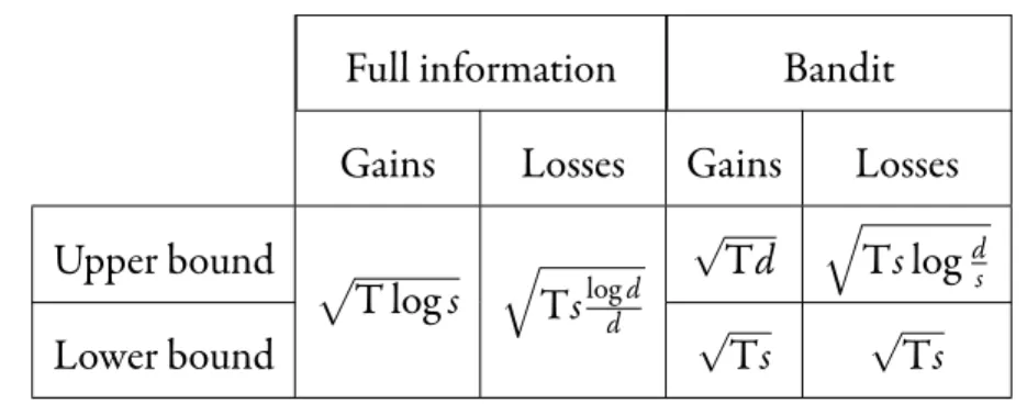
Le ChapitreVest tiré de l’article [KP16b] et étudie le problème de la minimisation du regret dans le cas où le joueur possède un ensemble fini d’actions, et avec l’hypo-thèse supplémentaire que les vecteurs de paiement possèdent au plus s composantes non-nulles. On établit, en information complète, que la borne optimale sur le regret est de l’ordre de√_{T log s (où T est le nombre d’étapes) lorsque les paiements sont des}

gains (c’est-à-dire lorsqu’ils sont positifs), et de l’ordre de√Tslog d_d (où d est le nombre d’actions) lorsqu’il s’agit de pertes (i.e. négatifs). On met ainsi en évidence une diffé-rence fondamentale entre les gains et les pertes. Dans le cadre bandit, on établit que la borne optimale pour les pertes est de l’ordre de√Ts à un facteur logarithmique près.

Le ChapitreVIest issu de l’article [KP16a] et porte sur l’approchabilité de Bla-ckwell avec observations partielles, c’est-à-dire que le joueur observe seulement des si-gnaux aléatoires. On construit des stratégies garantissant des vitesses de convergence de l’ordre de O(T−1/2_{)dans le cas de signaux dont les lois ne dépendent pas de}

l’ac-tion du joueur, et de l’ordre de O(T−1/3_{)dans le cas général. Cela établit qu’il s’agit}

là des vitesses optimales car il est connu qu’on ne peut les améliorer sans hypothèse supplémentaire sur l’ensemble cible ou la structure des signaux.

Le ChapitreVIIest tiré de l’article [KM14] et définit les stratégies de descente miroir en temps continu. On établit pour ces derniers une propriété de non-regret. On effectue ensuite une comparaison entre le temps continu et le temps discret. Cela offre une interprétation des deux termes qui constituent la borne sur le regret en temps discret : l’un vient de la propriété en temps continu, l’autre de la comparaison entre le temps continu et le temps discret.

Enfin, le ChapitreVIIIest indépendant et est issu de l’article [Kwo14]. On y établit une borne universelle sur les variations des fonctions convexes bornées. On obtient en corollaire que toute fonction convexe bornée est lipschitzienne par rapport à la métrique de Hilbert.

[KP16b] Joon Kwon and Vianney Perchet. Gains and losses are fundamentally dif-ferent in regret minimization : the sparse case. arXiv :1511.08405, 2016 (à pa-raître dansJournal of Machine Learning Research)

[KP16a] Joon Kwon and Vianney Perchet. Blackwell approachability with partial monitoring : Optimal convergence rates. 2016 (en préparation)

9 [KM14] Joon Kwon and Panayotis Mertikopoulos. A continuous-time approach to

online optimization. arXiv :1401.6956, 2014 (en préparation)

[Kwo14] Joon Kwon. A universal bound on the variations of bounded convex func-tions. arXiv :1401.2104, 2014 (à paraître dans Journal of Convex Analysis)

ABSTRACT

The manuscript is divided in two parts. The first consists in Chapters I to IV and offers a unified presentation of numerous known results as well as some new elements. We present in Chapter Ithe online linear optimization problem, then construct Mirror Descent strategies with varying parameters for regret minimization, and es-tablish in TheoremI.3.1a general bound on the regret guaranteed by the strategies. This result is fundamental, as most of the results from the first four chapters will be obtained as corollaries. We then deal with the extension to convex losses, and with the derivation of convex optimization algorithms from regret minimizing strategies.

Chapter II focuses on the case where the Decision Maker has a finite set from which he can pick his actions at random. The strategies from Chapter Iare easily transposed to this framework and we also obtain high-probability and almost-sure guarantees. We then review a few known strategies: Exponential Weights Algorithm, Smooth Fictitious Play, and Vanishingly Smooth Fictitious Play, which all appear as spe-cial cases of the strategies constructed in Chapter I. At the end of the chapter, we mention the multi-armed bandit problem, where the Decision Maker only observes the payoff of the action he has played. We study the EXP3 strategy, which is an adap-tation of the Exponential Weights Algorithm to this setting.

Chapter III is dedicated to the family of strategies called Follow the Perturbed Leader, which is defined using random perturbations. A recent survey [ALT16] mentions the fact that those strategies, although defined differently, actually belong to the family of Mirror Descent strategies from ChapterI. We give a detailed proof of this result.

Chapter IV aims at constructing Mirror Descent strategies for Blackwell’s approachability. We extend an approach proposed by [ABH11] that turns a regret minimizing strategy into an approachability strategy. Our construction is more general, as it provides bounds for a very large class of distance-like quantities which measure the “distance” to the target set and not only on the Euclidean distance to the target set. The unifying character of this approach is then illustrated by the construction of optimal strategies for online combinatorial optimization and internal/swap regretminimization. Besides, we prove that Blackwell’s strategy can be seen as a special case of Mirror Descent.

The second part of the manuscript contains the following four papers.

ChapterVis from [KP16b] and studies the regret minimization problem in the case where the Decision Maker has a finite set of actions, with the additional assump-tion that payoff vectors have at most s nonzero components. We establish, in the full information setting, that the minimax regret is of order√_{T log s (where T is the}

num-ber of steps) when payoffs are gains (i.e nonnegative), and of order√Tslog d_d (where d is the number of actions) when the payoffs are losses (i.e. nonpositive). This demon-strates a fundamental difference between gains and losses. In the bandit setting, we prove that the minimax regret for losses is of order√Ts up to a logarithmic factor.

ChapterVIis extracted from [KP16a] and deals with Blackwell’s approachability with partial monitoring, meaning that the Decision Maker only observes random sig-nals. We construct strategies which guarantee convergence rates of order O(T−1/2₎

in the case where the signal does not depend on the action of the Decision Maker, and of order O(T−1/3)in the case of general signals. This establishes the optimal rates in those two cases, as the above rates are known to be unimprovable without further assumption on the target set or the signalling structure.

ChapterVIIcomes from [KM14] and defines Mirror Descent strategies in con-tinuous time. We prove that they satisfy a regret minimization property. We then conduct a comparison between continuous and discrete time. This offers an inter-pretation of the terms found in the regret bounds in discrete time: one is from the continuous time property, and the other comes from the comparison between con-tinuous and discrete time.

Finally, ChapterVIIIis independent and is from [Kwo14]. We establish a uni-versal bound on the variations of bounded convex function. As a byproduct, we ob-tain that every bounded convex function is Lipschitz continuous with respect to the Hilbert metric.

[KP16b] Joon Kwon and Vianney Perchet. Gains and losses are fundamentally dif-ferent in regret minimization: the sparse case. arXiv:1511.08405, 2016 (to ap-pear inJournal of Machine Learning Research)

[KP16a] Joon Kwon and Vianney Perchet. Blackwell approachability with partial monitoring: Optimal convergence rates. 2016 (in preparation)

[KM14] Joon Kwon and Panayotis Mertikopoulos. A continuous-time approach to online optimization. arXiv:1401.6956, 2014 (in preparation)

[Kwo14] Joon Kwon. A universal bound on the variations of bounded convex func-tions. arXiv:1401.2104, 2014 (to appear in Journal of Convex Analysis)

Introduction 17

First part

29

I Mirror Descent for regret minimization 31

I.1 Core model . . . 31

I.2 Regularizers . . . 33

I.3 Mirror Descent strategies . . . 41

I.4 Convex losses . . . 44

I.5 Convex optimization . . . 45

II Experts setting 49 II.1 Model . . . 49

II.2 Mirror Descent strategies . . . 51

II.3 Exponential Weights Algorithm . . . 53

II.4 Sparse payoff vectors . . . 55

II.5 Smooth Fictitious Play . . . 58

II.6 Vanishingly Smooth Fictitious Play . . . 59

II.7 On the choice of parameters . . . 60

II.8 Multi-armed bandit problem . . . 61

III Follow the Perturbed Leader 65 III.1 Presentation . . . 65

III.2 Historical background . . . 66

III.3 Reduction to Mirror Descent . . . 66

III.4 Discussion . . . 69

IV Mirror Descent for approachability 71 IV.1 Model . . . 71

IV.2 Closed convex cones and support functions . . . 72

IV.3 Mirror Descent strategies . . . 76

15

IV.4 Smooth potential interpretation . . . 78

IV.5 Blackwell’s strategy . . . 78

IV.6 Finite action set . . . 82

IV.7 Online combinatorial optimization . . . 84

IV.8 Internal and swap regret . . . 89

Second part

95

V.2 When outcomes are gains to be maximized . . . 101

V.3 When outcomes are losses to be minimized . . . 104

V.4 When the sparsity level s is unknown . . . . 111

V.5 The bandit setting . . . 119

VI Approachability with partial monitoring 131 VI.1 Introduction . . . 131

VI.2 The game . . . 133

VI.3 Approachability . . . 135

VI.4 Construction of the strategy . . . 136

VI.5 Main result . . . 142

VI.6 Outcome-dependent signals . . . 153

VI.7 Discussion . . . 157

VI.8 Proofs of technical lemmas . . . 160

VII Continuous-time Mirror Descent 169 VII.1 Introduction . . . 169

VII.2 The model . . . 172

VII.3 Regularizer functions, choice maps and learning strategies . . . . 175

VII.4 The continuous-time analysis . . . 180

VII.5 Regret minimization in discrete time . . . 181

VII.6 Links with existing results . . . 185

VII.7 Discussion . . . 193

VIII A universal bound on the variations of bounded convex functions 197 VIII.1 The variations of bounded convex functions . . . 197

VIII.2 The Funk, Thompson and Hilbert metrics . . . 199

VIII.3 Optimality of the bounds . . . 201

Appendix

204

A Concentration inequalities 205

Bibliography 207

INTRODUCTION

Online learning

Online learning deals with making decisions sequentially with the goal of obtain-ing good overall results. Such problems have originated and have been studied in many different fields such as economics, computer science, statistics and information theory. In recent years, the increase of computing power allowed the use of online learning algorithms in countless applications: advertisement placement, web rank-ing, spam filterrank-ing, energy consumption forecast, to name a few. This has naturally boosted the development of the involved mathematical theories.

Online learning can be modeled as a setting where a Decision Maker faces Nature repeatedly, and in which information about his performance and the changing state of Nature is revealed throughout the play. The Decision Maker is to use the infor-mation he has obtained in order to make better decisions in the future. Therefore, an important characteristic of an online learning problem is the type of feedback the Decision Maker has, in other words, the amount of information available to him. For instance, in the full information setting, the Decision Maker is aware of everything that has happened in the past; in the partial monitoring setting, he only observes, after each stage, a random signal whose law depends on his decision and the state of Nature; and in the bandit setting, he only observes the payoff he has obtained.

Concerning the behavior of Nature, we can distinguish two main types of assump-tions. In stochastic settings, the successive states of Nature are drawn according to some fixed probability law, whereas in the adversarial setting, no such assumption is made and Nature is even allowed to choose its states strategically, in response to the previ-ous choices of the Decision Maker. In the latter setting, the Decision Maker is aiming at obtaining worst-case guarantees. This thesis studies adversarial online problems.

To measure the performance of the Decision Maker, a quantity to minimize or a criterion to satisfy has to be specified. We present below two of those: regret min-imization and approachability. Both are very general frameworks which have been successfully applied to a variety of problems.

Regret minimization

We present the adversarial regret minimization problem which has been used as a unifying framework for the study of many online learning problems: pattern recogni-tion, portfolio management, routing, ranking, principal component analysis, matrix learning, classification, regression, etc. Important surveys on the topic are [CBL06,

RT09,Haz12,BCB12,SS11].

We first consider the problem where the Decision Maker has a finite set of actions

ℐ = {1,…, d}. At each stage t ⩾ 1, the Decision Maker chooses an action i_t ∈ ℐ, possibly at random, then observes a payoff vector u_t ∈ [−1, 1]d_{, and finally gets a scalar}

payoff equal to uit

t. We assume Nature to be adversarial, and the Decision Maker is

therefore aiming at obtaining some guarantee against any possible sequence of payoff vectors(u_t)_t⩾1in[−1, 1]d_{. Hannan [Han57] introduced the notion of regret, defined}

as R_T =max i∈ℐ T 􏾜 t=1 ui t − T 􏾜 t=1 uit t,

which compares the cumulative payoff ∑T

t=1u

i_t

t obtained by the Decision Maker to

the cumulative payoff max_i∈ℐ∑T_t=1uithe could have obtained by playing the best fixed

action in hindsight. Hannan [Han57] established the existence of strategies for the Decision Maker which guarantee that the average regret _T1R_Tis asymptotically non-positive. This problem is also called prediction with expert advice because it models the following situation. Imagineℐ = {1,…, d}as a set of experts. At each stage t ⩾ 1, the Decision Maker has to make a decision and each expert give a piece of advice as to which decision to make. The Decision Maker must then choose the expert i_t to follow. Then, the vector u_t ∈ _Rd _{is observed, where u}i

t is the payoff obtained by

ex-pert i. The payoff obtained by the Decision Maker is therefore uit

t. The regret then

corresponds to the difference between the cumulative payoff of the Decision Maker and the cumulative payoff obtained by the best expert. The Decision Maker having a strategy which makes sure that the average regret goes to zero means that he is able to perform, asymptotically and in average, as well as any expert.

The theory of regret minimization has since been refined and developed in a num-ber of ways—see e.g. [FV97,HMC00,FL99,Leh03]. An important direction was the study of the best possible guarantee on the expected regret, in other words the study of the following quantity:

inf supE [RT],

where the infimum is taken over all possible strategies of the Decision Maker, the supremum over all sequences(u_t)_t⩾1of payoff vectors in[−1, 1]d_{, and the expectation}

introduction 19 its actions i_t. This quantity has been established [CB97, ACBG02] to be of order

√_{T log d, where T is the number of stages and d the number of actions.}

An interesting variant is the online convex optimization problem [Gor99,KW95,

KW97,KW01,Zin03]: the Decision Maker chooses actions z_t in a convex compact set𝒵 ⊂Rd_{, and Nature chooses loss functionsℓ}

t ∶ 𝒵 →R. The regret is then defined

by R_T = T 􏾜 t=1 ℓ_t(z_t) −min z∈𝒵 T 􏾜 t=1 ℓ_t(z).

The special case where the loss functions are linear is called online linear optimization and is often written with the help of payoff vectors(u_t)_t⩾1:

R_T =max z∈𝒵 T 􏾜 t=1 ⟨u_t|z⟩ − T 􏾜 t=1 ⟨u_t|z_t⟩ . (∗)

This will be the base model upon which Part I of the manuscript will be built.

Until now, we have assumed that the Decision Maker observes all previous payoff vectors (or loss functions), in other words, that he has a full information feedback. The problems in which the Decision Maker only observes the payoff (or the loss) that he obtains are called bandit problems. The case where the set of actions isℐ = {_1,…_{, d}}

is called the adversarial multi-armed bandit problem, for which the minimax regret is known to be of order√Td [AB09,ACBFS02]. The bandits settings for online con-vex/linear optimization has also attracted much attention [AK04,FKM05, DH06,

BDH+_{08] and we refer to [BCB12] for a recent survey.}

Approachability

Blackwell [Bla54,Bla56] considered a model of repeated games between a Deci-sion Maker and Nature with vector-valued payoffs. He studied the sets to which the Decision Maker can make sure his average payoff converges. Such sets are said to be approachableby the Decision Maker. Specifically, letℐand𝒥be finite action sets for the Decision Maker and Nature respectively,

Δ(ℐ) = {x= (xi₎

i∈ℐ ∈Rℐ+∣􏾜

i∈ℐ

xi_=1}

the set of probability distributions onℐ, and g ∶ ℐ × 𝒥 →Rd_{a vector-valued payoff}

•y₀

•y

𝒞

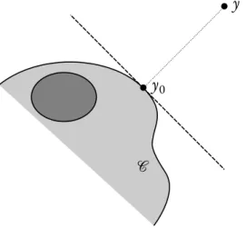
Figure 1. The hyperplane⟨y−y₀| ⋅ −y₀⟩ = 0 separates y and the set of all pos-sible expected vector payoffs when the Decision Maker plays at random according to probability distribution x(y)(represented in dark gray).

a strategy for the Decision Maker which guarantees that 1 T T 􏾜 t=1 g(i_t, j_t) −−−−→ T→+∞ 𝒞,

where i_tand j_tdenote the actions chosen at time t by the Decision Maker and Nature, respectively.

Blackwell provided the following sufficient condition for a closed set𝒞 ⊂ Rdto be approachable: for all y ∈ _Rd_{, there exists an Euclidean projection y}

0 of y onto𝒞,

and a probability distribution x(y) ∈Δ(ℐ)such that for all actions j∈ 𝒥of Nature,

⟨_Ei∼x(y)[g(i, j)] −y₀∣y−y₀⟩ ⩽0.

The above inequality is represented in Figure1. 𝒞is then said to be a B-set. When this is the case, the Blackwell strategy is defined as

x_t+1 =x(1 t t 􏾜 s=1 g(i_s, j_s)) then draw i_t+1 ∼x_t+1,

which means that action i_t+1 ∈ ℐis drawn according to probability distribution x_t+1 ∈

Δ(ℐ). This strategy guarantees the convergence of the average payoff _T1 ∑T

t=1g(it, jt)

to the set𝒞_{. Later, [Spi02] proved that a closed set is approachable if and only if it}

contains a B-set. In the case of a convex set𝒞, Blackwell proved that it is approachable if and only if it is a B-set, which is then also equivalent to the following dual condition:

∀y∈Δ(𝒥), ∃x∈Δ(ℐ), Ei∼x

introduction 21 This theory turned out to be a powerful tool for constructing strategies for on-line learning, statistics and game theory. Let us mention a few applications. Many variants of the regret minimization problem can be reformulated as an approacha-bility problem, and conversely, regret minimization strategy can be turned into ap-proachability strategy. Blackwell [Bla54] was already aware of this fundamental link between regret and approachability, which has since been much developed—see e.g. [HMC01,Per10,MPS11,ABH11,BMS14,Per15]. The statistical problem of cali-brationhas also proved to be related to approachability [Fos99,MS10,Per10,RST11,

ABH11,Per15]. We refer to [Per14] for a comprehensive survey on the relations be-tween regret, calibration and approachability. Finally, Blackwell’s theory has been applied to the construction of optimal strategies in zero-sum repeated games with in-complete information [Koh75,AM85].

Various techniques have been developed for constructing and analyzing approach-ability strategies. As shown above, Blackwell’s initial approach was based on Euclidean projections. A potential-based approach was proposed to provide a wider and more flexible family of strategies [HMC01,CBL03,Per15]. In a somewhat related spirit, and building upon an approach with convex cones introduced in [ABH11], we define in ChapterIVa family of Mirror Descent strategies for approachability.

The approachability problem has also been studied in the partial monitoring set-ting [Per11a,MPS11,PQ14,MPS14]. In ChapterVIwe construct strategies which achieve optimal convergence rates.

On the origins of Mirror Descent

In this section, we quickly present the succession of ideas which have led to the Mirror Descent algorithms for convex optimization and regret minimization. We do not aim at being comprehensive nor completely rigorous. We refer to [CBL06, Section 11.6], [Haz12], and to [Bub15] for a recent survey.

We first consider the unconstrained problem of optimizing a convex function f∶ Rd _{→Rwhich we assume to be differentiable:}

min

x∈Rdf(x).

We shall focus on the construction of algorithms based on first-order oracles—in other words, algorithms which have access to the gradient∇f(x)at any point x. Gradient Descent

The initial idea is to adapt the continuous-time gradient flow

̇

−γ_t∇f(x_t+1) •x_t • x_t+1 −_γt∇f(x_t) • x_t • x_t+1

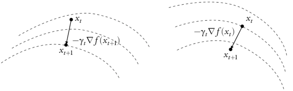
Figure 2. The Proximal algorithm on the left and Gradient Descent on the right There are two basic discretizations. The first is the proximal algorithm, which starts at some initial point x₁and iterates as

x_t+1 =x_t−γ_t∇f(x_t+1), (1) where γ_t is a step-size. The algorithm is said to be implicit because one has to find a point x_t+1satisfying the above equality in which x_t+1implicitly appears in∇f(x_t+1). One can see that the above relation can be rewritten

x_t+1 =arg max x∈Rd {f(x) + 1 2γ_t ‖x−xt‖ 2 2} . (2)

Indeed, the function x⟼f(x)+_2γ1

t‖x−xt‖ 2

2having at point xt+1a gradient equal to

zero is equivalent to Equation (1). The above expression (2) guarantees the existence of x_t+1and provides the following interpretation: point xt+1 corresponds to a

trade-off between minimizing f and being close to the previous iterate x_t. The algorithm can also be written in a variational form: x_t+1is characterized by

⟨γ_t∇f(x_t+1) +x_t+1−x_t|x−x_t+1⟩ ⩾0, ∀x∈_Rd_{. (3)}

The second discretization is the Euler scheme, also called the gradient descent algo-rithm:

x_t+1 =x_t−γ_t∇f(x_t), (4) which is said to be explicit because the point x_t+1 follows from a direct computation involving x_t and∇f(x_t), which are known to the algorithm. It can be rewritten

x_t+1 =arg min x∈Rd {⟨∇f(x_t)|x⟩ + 1 2γ_t ‖x−xt‖ 2 2}, (5)

introduction 23 which can be seen as a modification of the proximal algorithm (2) where f(x) has been replaced by its linearization at x_t. Its variational form is

⟨γ_t∇f(x_t) +x_t+1−x_t|x−x_t+1⟩ ⩾0, ∀x∈Rd_{. (6)}

Projected Gradient Descent

We now turn to the constrained problem min

x∈Xf(x),

where X is a convex compact subset ofRd_{. The gradient descent algorithm (4) can}

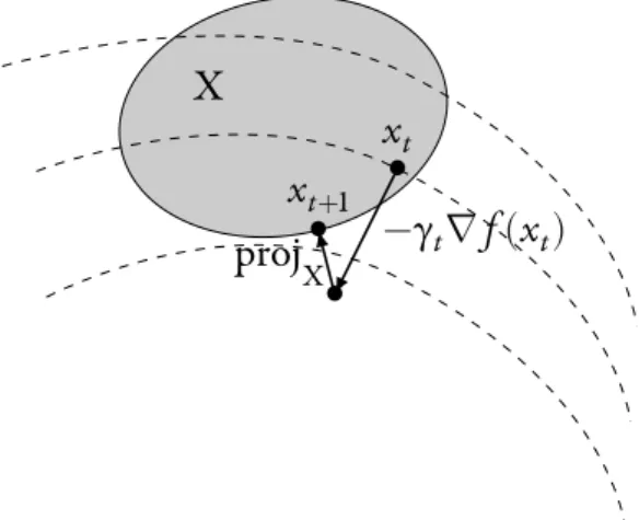
be adapted for this problem by performing a Euclidean projection onto X after each gradient descent step, in order to have all iterates x_tin the set X. This gives the projected gradient descentalgorithm [Gol64,LP66]:

x_t+1 =proj

X

{x_t−γ_t∇f(x_t)}, (7) which can rewritten as

x_t+1 =arg min x∈X {⟨∇f(x_t)|x⟩ + 1 2γ_t ‖x−xt‖ 2 2}, (8)

and has variational characterization:

⟨γ_t∇f(x_t) +x_t+1−x_t|x−x_t+1⟩ ⩾0, ∀x∈X, x_t+1 ∈X. (9) Typically, when the gradients of f are assumed to be bounded by M > 0 with re-spect to‖ ⋅ ‖

2(in other words, if f is M-Lipschitz continuous with respect to‖ ⋅ ‖2),

the above algorithm with constant step-size γ_t = ‖X‖ 2/M

√

T provides a M/√ T-optimal solution after T steps. When the gradients are bounded by some other norm, the above still applies but the dimension d of the space appears in the bound. For in-stance, if the gradients are bounded by M with respect to‖ ⋅ ‖

∞, due to the comparison

between the norms, the above algorithm provides after T steps a M√_d/T-optimal solution. Then, the following question arises: if the gradients are bounded by some other norm than‖ ⋅ ‖

2, is it possible to modify the algorithm in order to get a

guaran-tee that has a better dependency in the dimension? This motivates the introduction of Mirror Descent algorithms.

−γ_t∇f(x_t) • x_t • proj_X• x_t+1 X

Figure 3. Projected Subgradient algorithm Greedy Mirror Descent

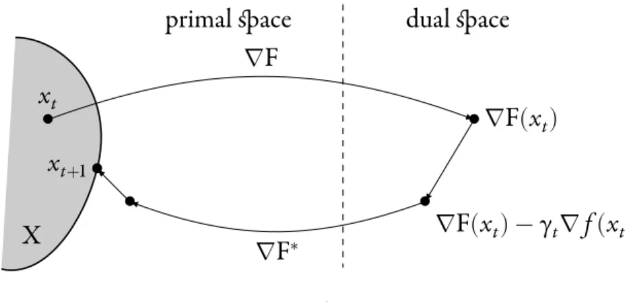
Let F ∶ _Rd _{→ Rbe a differentiable convex function such that ∇F ∶ R}d _{→ R}d

is a bijection. Denote F∗ _{its Legendre–Fenchel transform. Then, one can see that} (∇_F)−1 _{= ∇F}∗_{. We introduce the Bregman divergence associated with F:}

D_F(x′_{, x) =F(x}′_{) −F(x) − ⟨∇F(x)|x}′_{−x⟩, x, x}′ _∈Rd_,

which is a quadratic quantity that can be interpreted as a generalized distance. It pro-vides a new geometry which will replace the Euclidean structure used for the Pro-jected Gradient Descent (7). The case of the Euclidean distance can be recovered by considering F(x) = ₂1 ‖x‖2

2which gives DF(x

′_{, x) =} 1

2‖x′−x‖ 2

2. The Greedy Mirror

Descentalgorithm [NY83,BT03] is defined by replacing in the Projected Gradient Descent algorithm (8) the Euclidean distance₂1 ‖x−x_t‖2

2by the Bregman divergence

D_F(x, x_t):

x_t+1 =_{arg min}

x∈X

{⟨∇f(x_t)|x⟩ + 1

γ_tDF(x, xt)} . (10) This algorithm can also be written with the help of a gradient descent and a projection:

x_t+1 =arg min

x∈X

D_F(x,∇F∗_(∇F(x

t) −γt∇f(xt))) . (11)

The above expression of x_t+1 can be decomposed and interpreted as follows. Since

we have forgotten about the Euclidean structure, point x_tbelongs to the primal space whereas gradient∇f(x_t)lives in the dual space. Therefore, we cannot directly per-form the gradient descent x_t−γ_t∇f(x_t)as in (7). Instead, we first use the map∇F to get from x_tin the primal space to∇F(x_t)in the dual space, and perform the gradi-ent descgradi-ent there: ∇F(x_t) −γ_t∇f(x_t). We then use the inverse map∇F∗ _{= (∇F)}−1

introduction 25 • • x_t ∇F • ∇_F(x_t) • ∇F(x_t) −γ_t∇f(x_t) ∇F∗ • • x_t+1

primal space dual space

X

Figure 4. Greedy Mirror Descent to come back to the primal space: ∇F∗_(∇F(x

t) −γt∇f(xt)). Since this point may

not belong to the set X, we perform a projection with respect to the Bregman diver-gence D_F, and we get the expression of x_t+1from (11). Let us mention the variational expression of the algorithm, which is much more handy for analysis

⟨γ_t∇f(x_t) + ∇F(x_t+1) − ∇F(x_t)|x−x_t+1⟩ ⩾0, ∀x∈X, x_t+1 ∈X. (12) As initially wished, the Greedy Mirror Descent algorithm can adapt to different assumptions about the gradients of the objective function f. If f is assumed to be M-Lipschitz continuous with respect to a norm‖ ⋅ ‖, the choice of a function F which is K-strongly convex with respect to‖ ⋅ ‖guarantees that the associated algorithm with constant step-size γt =

√

LK/_M√_{T gives a M}√_L/_{KT-optimal solution after T}

steps, where L=max_x,x′_∈X{F(x) −F(x′)}.

There also exists a proximal version of Greedy Mirror Descent algorithm. It is called the Bregman Proximal Minimization algorithm and was introduced by [CZ92]. It is obtained by replacing in the proximal algorithm (2) the Euclidean distance by a Bregman divergence:

x_t+1 =_{arg min}

x∈X

{f(x) + 1

γ_tDF(x, xt)} . Lazy Mirror Descent

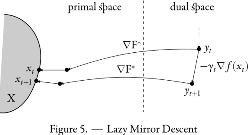
We now introduce a variant of the Greedy Mirror Descent algorithm (10) by mod-ifying it as follows. To compute x_t+1, instead of considering∇F(x_t), we perform the gradient descent starting from a point y_t(which will be defined in a moment) of the dual space: y_t−γ_t∇f(x_t). We then map the latter point back to the primal space via

∇F∗_{and then perform the projection onto X with respect to D}

•y_t • y_t+1 −γ_t∇f(x_t) ∇F∗ • ∇F∗ • • x_t • x_t+1

primal space dual space

X

Figure 5. Lazy Mirror Descent

Mirror Descentalgorithm, also called Dual Averaging [Nes09] which starts at some point x1 ∈X and iterates

x_t+1 =arg min

x∈X

D_F(x,∇F∗_(y

t−γt∇f(xt))) . (13)

Besides, we perform the update y_t+1 =yt−γt∇f(xt). If the algorithm is started with

y₁ = 0, we have y_t = −∑t−1

s=1γs∇f(xs)for all t ⩾ 1. Then, one can easily check that

(13) has the following simpler expression: x_t+1 =arg min x∈X {⟨ t 􏾜 s=1 γ_s∇f(x_s)∣x⟩ +F(x)}, (14) as well as a variational characterization:

⟨γ_t∇f(x_t) + ∇F(x_t+1) −y_t|x−x_t+1⟩, ∀x∈X, x_t+1 ∈X.

For the simple problem convex optimization that we are dealing with, this lazy algo-rithm provides similar guarantees as the greedy version (10)—compare [Nes09, Theo-rem 4.3] and [BT03, Theorem 4.1]. However, it has a computational advantage over the latter: the iteration in Equation (11) which gives x_t+1 from x_t involves the suc-cessive computation of maps∇F and∇F∗, whereas iterating (13) only involves the computation of∇F∗_{and the Bregman projection.}

Online Mirror Descent

Interestingly, the above convex optimization algorithms can be used for the on-line convex optimization problem presented above. The first approach of this kind was proposed by [Zin03], who adapted algorithm (7) to the framework where the Decision Maker faces a sequence(f_t)_t⩾1of loss functions, instead of a function f that

introduction 27 is constant over time. The Greedy Online Gradient Descent algorithm is obtained by simply replacing∇f(x_t)in (7) by∇f_t(x_t):

x_t+1 =proj

X

{x_t−γ_t∇f_t(x_t)}, which can alternatively be written

x_t+1 =arg min x∈X {⟨∇f_t(x_t)|x⟩ + 1 2γ_t ‖x−xt‖ 2 2} .

By introducing a function F satisfying the same assumptions as in the previous section, we extend the above to a family of Greedy Online Mirror Descent algorithms [Bub11,

BCB12]:

x_t+1 =arg min

x∈X

{⟨∇f_t(x_t)|x⟩ + 1

γ_tDF(x, xt)} . (15) Similarly, we can also define a lazy version [SS07,SS11,KSST12,OCCB15]:

x_t+1 =arg min x∈X {⟨ t 􏾜 s=1 γ_s∇f_s(x_s)∣x⟩ +F(x)} . (16) More generally, we can define the above algorithms by replacing the gradients

∇f_t(x_t)by arbitrary vectors u_t ∈ Rd_{which need not be the gradients of some}

func-tions f_t. For instance, the Lazy Online Mirror Descent algorithm can be written: x_t+1 =arg max x∈X {⟨ t 􏾜 s=1 u_s∣x⟩ −F(x)},

where F acts a regularizer. This motivates, for this algorithm, the alternative name: Follow the Regularized Leader[AHR08,RT09,AHR12]. This algorithm provides a guarantee on: max x∈X T 􏾜 t=1 ⟨u_t|x⟩ − T 􏾜 t=1 ⟨u_t|x_t⟩,

which is the same quantity as in Equation (∗), i.e. the regret in the online linear op-timization problem with payoff vectors(u_t)_t⩾1. An important property is that payoff vector u_t is allowed to depend on x_t, as it is the case in (16) where u_t = −γ_t∇f(x_t). This Lazy Online Mirror Descent family of algorithms will be our subject of study in ChaptersItoIV. Throughout Part I of the manuscript, unless mentioned otherwise, Mirror Descentwill designate the Lazy Online Mirror Descent algorithms.

CHAPTER I

MIRROR DESCENT FOR REGRET

MINIMIZATION

We present the regret minimization problem called online linear optimization. Some convexity tools are introduced, with a special focus on strong convexity. We then construct the family of Mirror Descent strategies with time-varying parameters and derive general regret guarantees in TheoremI.3.1. This result is central as most results in Part I will be obtained as corollaries. In Section I.4, we present the generalization to convex losses (instead of linear payoffs), and in SectionI.5, we turn the aforementioned regret minimizing strategies into convex optimization algorithms.

I.1. Core model

The model we present here is called online linear optimization. It is a repeated play between a Decision Maker and Nature. Let𝒱_{be a finite-dimensional vector space,} 𝒱∗ _{its dual space, and denote ⟨ ⋅ | ⋅ ⟩the dual pairing. 𝒱}∗ _{will be called the payoff}

space1_{. Let𝒵be a nonempty convex compact subset of𝒱, which will be the set of}

actions of the Decision Maker. At each time instance t⩾_{1, the Decision Maker} • chooses an action z_t ∈ 𝒵;

• observes a payoff vector u_t ∈ 𝒱∗_{chosen by Nature;} • gets a payoff equal to⟨u_t|z_t⟩.

Formally, a strategy for the Decision Maker is a sequence of maps σ = (σ_t)_t⩾1

where σ_t ∶ (𝒵 × 𝒱∗₎t−1 _{→ 𝒵. In a slight abuse of notation, σ}

1 will be regarded as an

element of𝒵. For a given strategy σ and a given sequence(u_t)_t⩾1of payoff vectors, the sequence of play(z_t)_t⩾1is defined by

z_t =σ_t(z₁, u₁,…, z_t−1, u_t−1), t⩾1.

1. The dimension being finite, it would be good enough to work inRd. However, we believe that the theoretical distinction between the primal and dual spaces helps with the understanding of Mirror Descent strategies.

Concerning Nature, we assume it to be omniscient. Indeed, our main result, Theo-remI.3.1, will provide guarantees that hold against any sequence of payoff vectors. Therefore, its choice of payoff vector u_tmay depend on everything that has happened before he has to reveal it. In particular, payoff vector u_t may depend on action z_t.

The quantity of interest is the regret (up to time T⩾1), defined by Reg T{σ,(ut)t⩾1} =maxz∈𝒵 T 􏾜 t=1 ⟨u_t|z⟩ − T 􏾜 t=1 ⟨u_t|z_t⟩, T⩾1.

In most situations, we simply write Reg

T since the strategy and the payoffs vectors

will be clear from the context. In the case where Nature’s choice of payoff vectors

(u_t)_t⩾1does not depend on the actions of the Decision maker (Nature is then said to be oblivious), the regret can be interpreted as follows. It compares the cumulative payoff

∑T

t=1⟨ut|zt⟩obtained by the Decision Maker to the best cumulative payoff∑ T

t=1⟨ut|z⟩

that he could have obtained by playing a fixed action z∈ 𝒵at each stage. It therefore measures how much the Decision Maker regrets not having played the constant strat-egy that turned out to be the best. When Nature is not assumed to be oblivious (it is then said to be adversarial), in other words, when Nature can react to the actions

(z_t)_t⩾1chosen by the Decision Maker, the regret is still well-defined and every result below will stand. The only difference is that the above interpretation of the regret is not valid.

The first goal is to construct strategies for the Decision Maker which guarantee that the average regret 1

TRT is asymptotically nonpositive when the payoff vectors

are assumed to be bounded. In SectionI.3we construct the Mirror Descent strate-gies and derive in TheoremI.3.1general upper bounds on the regret which yield such guarantees.

One of the simplest strategies one can think of is called Follow the Leader or Ficti-tious Play. It consists in playing the action which would have given the highest cumu-lative payoff over the previous stages, had it been played at each stage:

z_t ∈arg max

z∈𝒵

⟨􏾜t−1

s=1

u_s∣z⟩ . (I.1) Unfortunately, this strategy does not guarantee the average regret to be asymptotically nonpositive, even in the following simple setting where the payoff vectors are bounded. Consider the framework where 𝒱 = 𝒱∗ = R2_, 𝒵 = Δ₂ = {(z₁, z₂) ∈_R2

+∣z1+z2=1}and where the payoff vectors all belong to [0, 1]2_{. Suppose that Nature chooses payoff vectors}

u₁ = (21

0), u2 = ( 0

regularizers 33 Then, one can easily see that using the above strategy (I.1) gives for t⩾2, z_t = (1, 0)if tis even, and z_t = (0, 1)if t is odd. As a result, the payoff⟨u_t|z_t⟩is zero as soon as t⩾2. The Decision Maker is choosing at each stage, the action which gives the worst payoff. As far as the regret is concerned, since max_z∈𝒵∑T_t=1⟨ut|z⟩is of order T/2, the regret

grows linearly in T. Therefore, the average regret is not asymptotically nonpositive. This phenomenon is called overfitting: following too closely previous data may result in bad predictions. To overcome this problem, we can try modifying strategy (I.1) as

z_t =arg max z∈𝒵 {⟨ t−1 􏾜 s=1 u_s∣z⟩ −h(z)},

where we introduced a function h in order to regularize the strategy. This is the key idea behind the Mirror Descent strategies (which are also called Follow the Regularized Leader) that we will define and study in SectionI.3.

I.2. Regularizers

We here introduce a few tools from convex analysis needed for the construction and the analysis of the Mirror Descent strategies. These are classic (see e.g. [SS07,

SS11,Bub11]) and the proofs are given for the sake of completeness. Again,𝒱and

𝒱∗are finite-dimensional vectors spaces and𝒵is a nonempty convex compact subset of𝒱. We define regularizers, present the notion of strong convexity with respect to an arbitrary norm, and give three examples of regularizers along with their properties. I.2.1. Definition and properties

We recall that the domain dom h of a function h ∶ 𝒱 → R ∪ {+∞}is the set of points where it has finite values.

Definition I.2.1. A convex function h ∶ 𝒱 → _{R ∪ {+∞}} is a regularizer on𝒵if it is strictly convex, lower semicontinuous, and has 𝒵as domain. We then denote δ_h =max𝒵h−min𝒵hthe difference between its maximal and minimal values on𝒵.

Proposition I.2.2. Let h be a regularizer on 𝒵. Its Legendre–Fenchel transform h∗ ∶ 𝒱∗ _{→R ∪ {+∞}, defined by}

h∗(w) = sup

z∈𝒱

{⟨w|z⟩ −h(z)}, w∈ 𝒱∗_,

satisfies the following properties. (i) dom h∗ _{= 𝒱}∗_;

(ii) h∗_{is differentiable on𝒱}∗_;

(iii) For all w∈ 𝒱∗_,∇h∗_{(w) = arg max}

z∈𝒵{⟨w|z⟩ −h(z)}. In particular,∇h ∗_takes

values in𝒵.

Proof. (i) Let w ∈ 𝒱∗_{. The function z ⟼ ⟨w|z⟩ − h(z)equals−∞outside of 𝒵,}

and is upper semicontinuous on𝒵 which is compact. It thus has a maximum and h∗(w) < +∞.

(ii,iii) Moreover, this maximum is attained at a unique point because h is strictly convex. Besides, for z∈ 𝒱and w∈ 𝒱∗

z∈ ∂h∗(w) ⟺ w∈ ∂h(z) ⟺ z∈arg max

z′_∈𝒵

{⟨w|z′⟩ −h(z′)}, in other words,∂h∗(w) =arg max

z′_∈𝒵{⟨w|z

′_{⟩ −h(z}′_{)}. This argmax is a singleton as}

we noticed. It means that h∗is differentiable.

Remark I.2.3. The above proposition demonstrates that h∗ _{is a smooth}

approxima-tion of max_z∈𝒵⟨ ⋅ |z⟩ and that ∇h∗ is an approximation of arg max_z∈𝒵⟨ ⋅ |z⟩. They

will be used in SectionI.3in the construction and the analysis of the Mirror Descent strategies.

As soon as h is a regularizer, the Bregman divergence of h∗_{is well defined:}

D_h∗(w′, w) =h∗(w′) −h∗(w) − ⟨∇h∗(w)|w′−w⟩, w, w′ ∈ 𝒱∗.

This quantity will appear in the fundamental regret bound of TheoremI.3.1. As we will see below in PropositionI.2.8, by adding a strong convexity assumption on the regularizer h, the Bregman divergence can be bounded from above by a much more explicit quantity.

I.2.2. Strong convexity

Definition I.2.4. Let h ∶ 𝒱 → _{R ∪ {+∞}}be a function, ‖ ⋅ ‖ a norm on𝒱, and K>0. h is K-strongly convex with respect to‖ ⋅ ‖if for all z, z′ _{∈ 𝒱and λ∈ [0, 1],}

h(λz+ (1−λ)z′_{) ⩽λh(z) + (1−λ)h(z}′_{) −}Kλ(1−λ)

2 ‖z

′_−z‖2_{. (I.2)}

Proposition I.2.5. Let h ∶ 𝒱 → R ∪ {+∞}be a function, ‖ ⋅ ‖ a norm on𝒱, and K>0. The following conditions are equivalent.

(i) h isK-strongly convex with respect to‖ ⋅ ‖;

(ii) For all points z, z′ ∈ 𝒱and all subgradients w∈ ∂h(z), h(z′) ⩾h(z) + ⟨w|z′−z⟩ + K

2 ‖z

′_−z‖2_;

regularizers 35 (iii) For all points z, z′_{∈ 𝒱and all subgradients w∈ ∂h(z)and w}′ _{∈ ∂h(z}′_),

⟨w′−w|z′−z⟩ ⩾K‖z′−z‖2. (I.4) Proof. (i)⟹ _{(ii). We assume that h is K-strongly convex with respect to} ‖ ⋅ ‖_{. In}

particular, h is convex. Let z, z′ _{∈ 𝒱, w ∈ ∂h(z), λ ∈ (0, 1), and denote z}′′ ₌

λz+ (1−λ)z′_{. Using the convexity of h, we have} ⟨w|z′−z⟩ = ⟨w|z ′′_−z⟩ 1−λ ⩽ h(z′′) −h(z) 1−λ ⩽ 1 1−λ(λh(z) + (1−λ)h(z ′_{) −} Kλ(1−λ) 2 ‖z ′_−z‖2_−h(z)) =h(z′_{) −h(z) −} Kλ 2 ‖z ′_−z‖2_,

and (I.3) follows from taking λ→1.

(ii)⟹(i). Let z, z′ _{∈ 𝒱, λ ∈ [0, 1], denote z}′′ _{= λz+ (1−λ)z}′_{. If λ ∈ {0, 1},}

inequality (I.2) is trivial. We now assume λ∈ (0, 1). If z or z′_{does not belong to the}

domain of h, inequality (I.2) is also trivial. We now assume z, z′ _{∈ dom h. Then, z}′′

belongs to]z, z′_{[which is a subset of the relative interior of dom h. Therefore,∂h(z}′′₎

is nonempty (see e.g. [Roc70, Theorem 23.4]). Let w∈ ∂h(z′′). We have

⟨w|z−z′′_{⟩ ⩽h(z) −h(z}′′_{) −} K 2 ‖z−z ′′_‖2 ⟨w|z′−z′′⟩ ⩽h(z′) −h(z′′) − K 2 ‖z ′_−z′′_‖2_.

By multiplying the above inequalities by λ and 1−λ respectively, and summing, we get

0⩽_λh(z) + (₁−_λ)h(z′) −h(z′′) − K

2 (λ‖z−z

′′_‖2_{+ (}

1−_λ) ‖z′−z′′‖2) .

Using the definition of z′′_{, we have z−z}′′ _{= (1−λ)(z}′_{−z)and z}′_−z′′ _=λ(z′_−z).

The last term of the above right-hand side is therefore equal to K

2 (λ(1−λ)2‖z

′_−z‖2_{+ (1−λ)λ}2_‖z′_−z‖2_{) =} Kλ(1−λ)

2 ‖z

′_−z‖2_,

and (I.2) is proved.

(ii)⟹(iii). Let z, z′ _{∈ 𝒱, w∈ ∂h(z)and w}′ _{∈ ∂h(z}′_{). We have}

h(z′) ⩾h(z) + ⟨w|z′−z⟩ + K 2 ‖z ′_−z‖2 _(I.5) h(z) ⩾h(z′) + ⟨w′|z−z′⟩ + K 2 ‖z ′_−z‖2_. (I.6)

Summing both inequalities and simplifying gives (I.4).

(iii) ⟹ (ii). Let z, z′ ∈ 𝒱. If ∂h(z) is empty, condition (ii) is automatically satisfied. We now assume∂h(z) ≠ ∅. In particular, z ∈ dom h. Let w ∈ ∂h(z). If h(z′_{) = +∞, inequality (I.3) is satisfied. We now assume z}′ _{∈ dom h. Therefore,}

we have that]z, z′_{[is a subset of the relative interior of dom h. As a consequence, for}

all points z′′ _{∈]z, z}′_{[, we have∂h(z}′′_{) ≠ ∅(see e.g. [Roc70, Theorem 23.4]). For all}

λ∈ [0, 1], we define z_λ =z+λ(z′_{−z). Using the convexity of h, we can now write,}

for all n⩾1, h(z′) −h(z) =􏾜n k=1 h(z_k/n) −h(z(k−1)/n) ⩾ n 􏾜 k=1 ⟨w(k−1)/n∣zk/n−z(k−1)/n⟩,

where w₀ = wand w_k/n ∈ ∂h(zk/n)for k ⩾ 1. Since zk/n−z(k−1)/n = n1(z′ −z)for

k⩾1, subtracting⟨w|z′−z⟩we get h(z′) −h(z) − ⟨w|z′−z⟩ ⩾ 1 n n 􏾜 k=1 ⟨w(k−1)/n−w∣z′−z⟩ .

Note that the first term of the above sum is zero because w= w₀. Besides, for k ⩾_2,

we have z′_−z= n

k−1(z(k−1)/n−z). Therefore, and this is where we use (iii),

h(z′_{) −h(z) − ⟨w|z}′_{−z⟩ ⩾ 􏾜}n k=2 1 k−1⟨w(k−1)/n−w∣z(k−1)/n−z⟩ ⩾_K􏾜n k=2 1 k−1∥z(k−1)/n−z∥ 2 = K‖z ′_−z‖2 n2 n 􏾜 k=2 (k−1) −−−−→ n→+∞ K 2 ‖z ′_−z‖2 , and (ii) is proved.

Similarly to usual convexity, there exists a strong convexity criterion involving the Hessian for twice differentiable functions.

Proposition I.2.6. Let‖ ⋅ ‖be a norm on𝒱,K >0, and F ∶ 𝒱 → Ra twice differen-tiable function such that

⟨∇2_{F(z)u∣u⟩ ⩾K‖u‖}2_{, z∈ 𝒱, u∈ 𝒱.}

regularizers 37 Proof. Let z, z′ _{∈ 𝒱. Let us prove the condition (ii) from Proposition I.2.5. We}

define

ϕ(λ) =F(z+λ(z′−z)), λ∈ [0, 1].

By differentiating twice, we get for all λ∈ [_{0, 1}]_:

ϕ′′(_λ) = ⟨∇2_F(z+λ(z′_−z))(z′_−z)∣z′_{−z⟩ ⩾K‖z}′_−z‖2_.

There exists λ0 ∈ [0, 1]such that ϕ(1) =ϕ(0) +ϕ′(0) +ϕ′′(λ0)/2. This gives

F(z′_{) =ϕ(1) =ϕ(0) +ϕ}′_{(0) +} ϕ′′(λ0)

2 ⩾F(z) + ⟨∇F(z)|z

′_{−z⟩ +} K

2 ‖z

′_−z‖2_,

and (I.3) is proved.

Lemma I.2.7. Let‖ ⋅ ‖a norm on𝒱,K > 0 and h, F ∶ 𝒱 → R ∪ {+∞}two convex functions such that for all z∈ 𝒱,

h(z) =F(z) or h(z) = +∞.

Then, ifF is K-strongly convex with respect to‖ ⋅ ‖, so is h.

Proof. Note that for all z∈ 𝒱_{, F}(z) ⩽h(z)_{. Let us prove that h satisfies the condition}

from DefinitionI.2.4. Let z, z′ _{∈ 𝒱, λ∈ [0, 1]and denote z}′′ _{=λz+ (1−λ)z}′_{. Let}

us first assume that h(z′′_{) = +∞. By convexity of h, either h(z)or h(z}′_{)is equal to} +∞_{, and the right-hand side of (I.2) is equal to}+∞_{. Inequality (I.2) therefore holds.}

If h(z′′_{)is finite,} h(z′′) =F(z′′) ⩽λF(z) + (1−λ)F(z′) −Kλ(1−λ) 2 ‖z ′_−z‖2 ⩽λh(z) + (1−λ)h(z′) −Kλ(1−λ) 2 ‖z ′_−z‖2_,

and (I.2) is proved.

For a given norm‖ ⋅ ‖on𝒱, the dual norm‖ ⋅ ‖_∗on𝒱∗_{is defined by} ‖w‖_∗ = sup

‖_z‖⩽1

|⟨w|z⟩| .

Proposition I.2.8. Let K > 0 and h ∶ 𝒱 → _{R ∪ {+∞}}be a regularizer which we assume to beK-strongly convex function with respect to a norm‖ ⋅ ‖on𝒱. Then,

D_h∗(w′, w) ⩽ 1

2K‖w

′_−w‖2

∗, w, w