Vision-based navigation in low earth orbit

HAL Id: hal-01304728

https://hal.inria.fr/hal-01304728

Submitted on 20 Apr 2016

HAL is a multi-disciplinary open access

archive for the deposit and dissemination of

sci-entific research documents, whether they are

pub-lished or not. The documents may come from

teaching and research institutions in France or

abroad, or from public or private research centers.

L’archive ouverte pluridisciplinaire HAL, est

destinée au dépôt et à la diffusion de documents

scientifiques de niveau recherche, publiés ou non,

émanant des établissements d’enseignement et de

recherche français ou étrangers, des laboratoires

publics ou privés.

Vision-based navigation in low earth orbit

Aurelien Yol, Eric Marchand, François Chaumette, Keyvan Kanani, Thomas

Chabot

To cite this version:

Aurelien Yol, Eric Marchand, François Chaumette, Keyvan Kanani, Thomas Chabot. Vision-based

navigation in low earth orbit. Int. Symp. on Artificial Intelligence, Robotics and Automation in

Space, i-SAIRAS’16, Jun 2016, Beijing, China. �hal-01304728�

ABSTRACT

This paper presents and compares two vision-based navigation methods for tracking space debris in a low Earth orbit environment. This work is part of the RemoveDEBRIS1 project. The proposed approaches rely on a frame to frame model-based tracking in order to obtain the complete 3D pose of the camera with respect to the target. The proposed algorithms robustly combine points of interest and edge features, as well as color-based features if needed. Experimental results are presented demonstrating the robustness of the approaches on synthetic image sequences simulating a CubeSat satellite orbiting the Earth. Finally, both methods are compared in order to specify what could be the best choice for the future of the RemoveDEBRIS mission.

1 INTRODUCTION

Since the beginning of the space era in 1957, the number of missions has incredibly increased. Unfortunately, it has also progressively generated a huge amount of debris that are still orbiting the Earth. Today, space agencies feel more and more concerned about Earth orbital environment cleaning since they realize those debris represent a big threat due to the high risk of collision that could, among safety issues, damage operational satellites [8]. To investigate solutions to this issue, various projects aim to actively remove debris objects by catching them. Among these projects, is the RemoveDEBRIS project co-funded by the European Union and members of European space industry. In a first stage, the RemoveDEBRIS mission will consist of catching two miniaturized satellites (CubeSats DS-1 and DS-2 produced by the Surrey Space Centre) that will be previously ejected from a microsatellite called RemoveSat, itself released from the International Space Station (ISS). Then, the CubeSats will be used as targets instead of actual debris. This debris removal demonstration will

1

This work is supported by the European Commission FP7-SPACE-2013-1 (project 607099) « RemoveDEBRIS – A Low Cost Active Debris Removal Demonstration Mission », a consortium partnership project consisting of: Surrey Space Centre (University of Surrey), SSTL, Airbus DS, Airbus SAS, Airbus Ltd, ISIS, CSEM, INRIA, and Stellen-Bosh University.

include net capture, harpoon capture and vision-based navigation using standard camera and LiDAR [9]. In the literature, several works propose approaches based on active sensors, such as LiDAR, for space rendezvous and docking missions [11]. Those approaches have proved to be efficient in situations where lighting conditions can be tricky due to directional sunlight resulting in high specularities and shadows. However, LiDAR are known to be generally expensive and rather heavy sensors. Furthermore, it also has a limited range and accuracy, and it cannot take the advantage of using potential texture information available on the target surface in order to improve the navigation process.

In this paper, we focus on the vision-based navigation part of the RemoveDEBRIS mission using a single standard RGB camera. Based on the knowledge of the 3D model of the target, estimating the complete 3D pose of the camera with respect to this target has always been an ongoing issue in computer vision and robotics applications [16]. For instance, regarding space applications, [1, 5] use model-based tracking approaches for space rendezvous with space target or debris. Common approaches try to solve this problem by using texture [2], edge features [1, 3, 4, 5], or color or intensity features [6, 7, 15]. The algorithms proposed in this paper provides a robust approach relying on a frame to frame tracking that align the projection of the 3D model of the target with observations made in the image by combining edges, point of interest and color-based features [14, 10]. Moreover, one of the presented method relies on the use of a 3D rendering engine to manage the projection of the model and to determine the visible and prominent edges from the rendered scene, while the other method is based on a hand-made 3D model but does not require any complex rendering process. The paper is organized as follow: in a first stage, the general issues of the model-based tracking problem are recalled. Then, we describe how to combine edges features with keypoints and color-based features by considering two different model-based tracking approaches. The first approach only relies on the use of a CPU, while the second takes the advantage of using a graphics processing unit (GPU). Finally, experimental results are presented on synthetic image

VISION-BASED NAVIGATION IN LOW EARTH ORBIT

*Aurelien Yol

, Eric Marchand

, Francois Cha umette

,

Keyvan Kanani

, Thoma s Chabot

sequences where comparisons are done between both approaches.

2 MODEL-BASED TRACKING

As stated before, our problem is restricted to model-based tracking where the considered 3D model is composed of a CAD representation of the target. In this paper, the model-based tracking part relies on a non-linear minimization of the reprojection error [16] where the general issue is to estimate the complete 3D pose of the camera with respect to the target # 𝐌$ by

minimizing the error ∆ between a set of measured data

𝑠'∗ (usually the position of a set of geometrical features

in the current image) and the same features projected in the image plane according to the current pose 𝑠' 𝒓 :

∆(𝐫) = 𝜌(𝑠' 𝐫 − 𝑠'∗)0 1

234

(1)

where 𝜌 is a robust estimator [12], which reduces the sensitivity to outliers (M-estimation) and 𝐫 is a vector-based representation of # 𝐌$ ( # 𝐌$ is the

homogeneous 4x4 matrix that represents the position of the object in the camera frame).

A common way of applying M-estimation is the Iteratively Reweighted Least Squares (IRLS) method. It converts the M-estimation problem into a least-squares one where the error to be regulated to zero is defined as:

𝐞 = 𝐃(𝐬 𝐫 − 𝐬∗_{) (2)}

where 𝐃 is a diagonal weighting matrix whose each coefficient gives the confidence on each feature. Their computation is based on M-estimators [3, 4].

Then, by considering an iterative least square approach given by:

𝒗 = − 𝜆 𝐃𝐋𝒔 <𝐞 (3)

where 𝑣 is the velocity screw applied to the virtual camera position and 𝐋𝒔 is the image Jacobian related

to 𝐬 defined such that 𝐬 = 𝐋𝒔𝒗. The 3D pose of the

camera can be iteratively updated from the computed displacement 𝒗 by applying an exponential map. More precisely, the resulting pose is given by:

𝐌

#>?@

$ = 𝐌#> $ exp (𝒗) (4)

where 𝑘 denotes the number of iterations in the minimization process.

While considering model-based tracking, it is important to decide what are the features 𝐬 to be used in order to define the error criterion (1). In this paper, we consider two model-based tracking methods that use a combination of geometrical edge-based features with keypoints features, and also color features along silhouette edges.

2.2 CPU-Based Model-Based Tracker

The first considered model-based tracking method relies only on a central processing unit (CPU), which is particularly appealing for space applications, thanks to the use of a simple hand-made CAD model. Furthermore, only edge-based features and keypoint features are used to define the error criterion (1). Considering different kind of features allows to benefit from their complementarity and to overcome the limitations of a single feature-based approach. In order to use them in the non-linear process presented in the previous section, the error ∆ to be minimized has to be rewritten according to the considered features. For this first method, it is defined as:

∆ = 𝑤F∆F+ 𝑤H∆H (5)

where ∆F refers to the geometrical edge-based error

and ∆H to the error relying on the keypoint features.

Respectively, 𝑤F and 𝑤H are the weighting parameters

used to control the influence of each set of features. Finally, to include the combination of the different features in the minimization process, the idea (as proposed in [10]) is to stack ∆Fand ∆H in a single

global error vector 𝐞 . Then, their corresponding Jacobian is also stacked and both are used as defined in (2) and (3).

Figure 1: Model-based tracking principle considering the case of edge and keypoint features. Edge-based features

From the knowledge on the 3D model of the target, a potential option is to use its silhouette to define features to rely on. Thus and as defined in (5), the first features we consider for this method are edge-based features. As in [3, 4], the edges that are considered correspond to the projection of the CAD model of the target, using the current camera pose 𝐫 . More precisely, the edges corresponding to the visible polygons of the model are considered in the minimization process. That is why this approach requires a simplified version of the 3D model that only contains polygons with visible edges (in term of gradient in the image). Furthermore, the visibility process has to be well defined in order to not consider

Current model position si(r) xp * i xg * i xg_(r) i xp_(r) i O y x θ li(r) d Measured position si*

edges that are hidden by other polygons. Neglecting the two above issues would result in adding extra outliers in the minimization process and consequently wrongly estimating the 3D pose of the camera. Once the visible edges of the model are projected in the image, each single line 𝑙 is sampled giving the set

of initial image points { 𝐱_'F}_'34MN. Each initial points is then tracked in order to determine the set of corresponding measured features { 𝐱_'F∗}_'34MN . As in [3], tracking is performed via a 1D search along the normal to the projection of the line𝑙' 𝐫 which is

associated to the point 𝐱_'F (see Figure 1). As a result, the error criterion ∆F referred as the edge-based

features error is defined as:

∆F(𝐫) = 𝜌F(𝑑P(𝑙' 𝐫 , 𝐱'F∗))0 1N

234

(6)

where 𝜌F is a robust estimator and 𝑑P(𝑙' 𝐫 , 𝐱'F∗) is

the distance between the forward projection of the line

𝑙' 𝐫 of the 3D model of the target and the desired

point features 𝐱_'F∗. Finally, the Jacobian of the distance of a point to a line is used (its analytic form is given in [3]).

Keypoint-based features

With a vision sensor and by considering that the target is potentially textured in the image, we have the possibility to use this information in order to improve the robustness of our navigation process. This is the reason why the considered methods also rely on keypoint-based features. Chosen keypoints are Harris corners that are tracked over the image sequence with the KLT algorithm [13]. Thus, the criterion error ∆H

refers here to the distance between 𝐱_'H 𝐫 , the position of the initial extracted keypoints 𝐱_'H with respect to the camera pose 𝐫, and their tracked position for each frame of the sequence 𝐱_'H∗ (see Figure 1).

∆H(𝐫) = 𝜌H( 𝐱'H 𝐫 − 𝐱'H∗)0 1R

234

(7)

where 𝜌H is once again a robust estimator.

Regarding 𝐱_'H 𝐫 , let us recall that for this first method we consider a simplified version of the 3D model of the target where keypoint are supposed to be detected on planar polygons belonging to the model. Thus, the displacement between the initial feature position and the tracked one can be specified by an homography. Then 𝐱_'H 𝐫 can be related to the initial position 𝐱_'Hof the keypoint by:

𝐱'H 𝐫 = α 𝐊UV4 𝐇 𝐊U 𝐱'H (8)

where 𝐊U is the calibration matrix associated to the intrinsic camera parameters 𝜉 , and 𝐇 is the

homography (up to a scale factor α) obtained from the 3D camera motion 𝐌#YZY[

#> _{computed between the} initial camera pose #YZY[ 𝐌$ and the current camera

pose #> 𝐌$ : 𝐇 = 𝐑_ ']'^ + 𝐭']'^ _ 𝑑 ']'^ ']'^ b 𝒏 (9)

where _ 𝐑']'^ and _ 𝐭']'^ are the rotation matrix and

translation vector extracted from the displacement

𝐌#YZY[ #> _{. Furthermore, 𝒏} ']'^ _{and 𝑑}

']'^ _{are the normal}

and distance to the origin of the planar polygon which

𝐱_'H 𝐫 belongs to. It is expressed in the initial camera

frame # 𝐌$']'^.

Finally, the Jacobian considering the coordinates of points is used and given by:

𝐋H= 𝐊U −1 𝑍 0 𝑥 𝑍 𝑥𝑦 −(1 + 𝑥 0_{) 𝑦} 0 −1 𝑍 𝑦 𝑍 (1 + 𝑦0) 𝑥𝑦 −𝑥 (10)

where (𝑥, 𝑦) are the normalized coordinates of the image point 𝐱_'H 𝐫 , and Z its corresponding depth obtained by: 1 𝑍 = 𝑑 − 𝐭']'^ _ b _𝒏 ']'^ ']'^ ( 𝐑_']'^ _ _𝒏 ']'^ ₎ b _𝐱 ' H _𝐫 . (11)

2.3 GPU-Based Model-Based Tracker

For the second considered model-based tracking method, we take the advantage of using a low-end graphics processing unit (GPU) to improve the vision-based navigation. Furthermore, in addition to edge-based features and keypoint features that were used in the previous method, we also consider color-based features. As a result, the error ∆ to be minimized has to be rewritten as:

∆ = 𝑤F∆F+ 𝑤H∆H+ 𝑤#∆# (12)

where ∆F and ∆H still refer to the geometrical

edge-based and keypoint-edge-based errors, with 𝑤Fand 𝑤H their

corresponding weighting parameters. ∆# is the

color-based features error with its associated weighting parameter 𝑤#.

Edge-based features

With respect to the previous method, the error criterion ∆F remains the same (see (6)). However, the determination of the edges to be considered is slightly different. In the approach proposed in [10] and used here, the CAD model of the target is rendered, according to the camera pose 𝐫 , by using a 3D rendering engine (in our case OpenSceneGraph). This allows to process the corresponding depth map of the scene in order to extract, via a Laplacian filter, the prominent edges of the projected model that will define the new set of initial point features { 𝐱_'F}_'34MN .

Tracking phase remains the same but as we are now dealing with a much complex 3D model, points are not associated anymore with any polygon. As a result, control points are processed independently and a 3D line 𝑙' is computed for each 𝐱'F (in blue on Figure 2).

Keypoint-based features

As for the keypoints, the feature-based error criterion

∆H remains the same (see (7)). However, with respect

to the previous method where polygons could contain several point features, we here have to take into account that every point may belong to a different polygon, due the potential complexity of the 3D model. Consequently, the way how 𝐱_'H 𝐫 and its corresponding depth Z are computed has to be changed in order to avoid unnecessary time processing. As in [10] we take the advantage of using the GPU and more particularly the rendered depth map to back-project the initial detected keypoints { 𝐱_'H}_'34MR on the model, which gives the set of corresponding 3D points { 𝐗_'H}_'34MR . These 3D points are then projected with the value of the camera pose 𝐫 and each point

𝐱_'H 𝐫 can be redefined as:

𝐱'H 𝐫 = 𝑝𝑟(𝐗'H, 𝐫) (13)

where 𝑝𝑟(𝐗_'H, 𝐫) is the perspective projection operator. Finally, the current depth value _ 𝑍 is computed by considering the current camera displacement 𝐌#YZY[

#> _. 𝐱'H _ _{= 𝐌} #YZY[ #> 𝐱 ' H ']'^ _{. (14)}

Note that the current depth value _ 𝑍 could also be

obtained by rendering the scene at the current pose

𝐌

#> _{$ and then using the corresponding depth map.} However, this solution has not been considered since it requires too much time to process the data.

Color-based features

One last improvement that has been added to this later approach in order to robustify the navigation process is to also consider color-based features. The idea is to use the prominent edges that have been extracted to compute the edge-based error criterion ∆F in order to

characterize the separation between the silhouette of the projected 3D model and the background by relying on color information [15, 10].

The principle is to compute local color statistics (RGB means 𝐈'm and 𝐈'n and covariances 𝐑'm and 𝐑n' where O

is the object and B the background) on both sides along the normal 𝒏' to the projected model silhouette edges { 𝐱_'F}_'34MN , regularly sampled in 𝐱',q# points up to

a distance 𝐿 (see Figure 2). These statistics are then mixed according to a fuzzy membership rule [17], giving the mean 𝐈' (𝐫) and covariance 𝐑' (𝐫) where

𝐈' (𝐫) is defined as the measured color value for 𝐱',q# .

Consequently, we can define the error 𝐞',q# 𝐫 as:

𝐞',q# 𝐫 = 𝐈' 𝐫 − 𝐈(𝐱',q# ) (15)

and the general error criterion ∆# can be re-written as:

∆#(𝐫) = 𝜌#( 𝐞',q# 𝐫 b𝐑' (𝐫)V4𝐞',q# 𝐫 ) q

'

(16) where 𝜌#, as for 𝜌H and 𝜌F, is a robust estimator based

on a Tukey M-Estimator.

For more accuracy and temporal smoothness, [15] and [10] also propose to introduce a temporal consistency by integrating the color statistics computed on the previous frame s 𝐈 for the silhouette edge point 𝐱'F 𝐫_

at the first iteration of the minimization process. With a weighting factor (0 < α < 1 ), it gives 𝐞',q# 𝐫 =

α𝐈' 𝐫 + (1 − 𝛼)( 𝐈s ' 𝐫 − 𝐈 𝐱',q# ). For the detailed

computation of the corresponding interaction matrix, see [17].

Finally, let us note that in case an RGB camera would not be available, it is still possible to use this approach with intensity only images. Indeed, color statistics defined above could still be computed by considering one image component only, that is, the intensity level for grey images.

Figure 2: Model-based tracking principle considering the case of color features.

3 EXPERIMENTAL RESULTS

The proposed methods have been validated on two synthetic image sequences where ground truth data are available to validate the quality of our vision-based navigation process. Both sequences simulate a CubeSat (DS-2) orbiting the Earth at different altitudes. The CubeSat DS-2 3D model has been generated by the Surrey Space Centre and provided by Airbus Defence and Space. The sequences have been generated via the 3D graphics and animation software Blender and the Earth has been textured using real satellite images available from NASA. Considered images dimensions are 640x480.

Structure of the target

The structure of the CubeSat DS-2 that will be used for the RemoveDEBRIS mission can be seen on Figure 3. It has avionics throughout the structure

Current model position si(r) xc i,j xg_(r) i Object Background _O y x θ li(r) ,

{

}

and four deployable panels at the bottom in the shape of a cross. The panels have no specific function except to make the CubeSat looking more like an actual satellite, so that the vision-based navigation is performed close to real conditions. Its dimensions (panels excluded) are 0.1m x 0.1m x 0.227m.

Figure 3: CubeSat DS-2 structure (image from [9]).

On Figure 4.a, we can see the CAD model used for the GPU-based approach. It is a wireframe representation of the model generated by the Surrey Space Center. The model is fully detailed and composed by many triangles. On the other side, the CAD model that is used for the CPU-based approach has been manually re-designed from the detailed model in order to contain only visible edges in terms of gradient in the image. There is no triangle in this simplified version, and the visible polygons on Figure 4.b directly represent the edges that will be used to define the edge-based and keypoint-based criterion errors (6) and (7). Models differences can also be seen on Figures 5.d and 6.d.

(a) (b)

Figure 4: 3D model used for the GPU-based MBT (a) and for the CPU-based MBT (b).

Case 1: case of a geosynchronous orbit

In the first sequence (see Figures 5 and 6), the considered target is on a geosynchronous orbit. It has an angular speed that creates rotational motions in the camera frame. However, the distance to the camera remains the same over the sequence. We have also considered different lighting conditions to simulate day and night (where the background also changes) in order to prove the robustness of our methods whatever the situation. The full video result for the GPU-based approach is available at: https://youtu.be/H9XKDaQEVbU, and for the CPU-based approach at: https://youtu.be/Gr78pmRPKOA.

(a) Image 0 (b) Image 680

(c) Image 2145 (d) Image 2602

Figure 5: Vision-based navigation of a CubeSat DS-2 for the first sequence of a geosynchronous orbit,

using the GPU-based approach.

(a) Image 0 (b) Image 680

(c) Image 2145 (d) Image 2602

Figure 6: Vision-based navigation of a CubeSat DS-2 for the first sequence of a geosynchronous orbit,

using the CPU-based approach. .

Figure 7: 3D poses estimated for the first sequence of a geosynchronous orbit (translation in meters and

rotation in radians). -2.5 -2 -1.5 -1 -0.5 0 0.5 1 1.5 2 2.5 3 0 500 1000 1500 2000 2500 3000 Cube Sat pos e i n the c ame ra frame Frame number X (m) Y (m) Z (m) rX (rad) rY (rad) rZ (rad)

CPU-based MBT

GPU-based MBT

RMSE Translation 0.0056 (m) 0.0039 (m) RMSE Rotation 0.0087 (rad) 0.0098 (rad)

Mean Time 69 ms 290 ms

Mean Nb. Feat. ≈800 ≈420

Table 1: First sequence: Root mean square errors (in meters for the translation and radians for the rotation), mean time and mean number of features

per frame obtained for the estimated navigation values.

For this first sequence, both methods have been able to perfectly track the target. The estimated trajectory, which is fairly the same for both methods, is accurate and smooth (see Figure 7). Furthermore, according to the collected ground truth data, our vision-based navigation provides precise pose estimation with an RMSE that is less than 1cm on the translation and about 2deg on the rotation (see Table 1). However, Table 1 also shows that the GPU-based solution is about 4 times more consuming than the CPU-based one (70ms per frame vs 290ms per frame), while considering twice less features (≈800 vs ≈420). This is mainly

due to the fact that, for the GPU-based approach, we are using a 3D rendering engine with a much more complex 3D representation of the target. Finally, on Figures 8 and 9, we can see the norm of the translational and rotational errors to the ground truth, which also shows where the algorithms encounter difficulties. Around frame 2200 for example, and for both approaches, the precision on the 3D pose estimation decreases a bit. The reason is that the panels of the target are orthogonally aligned with the focal axis of the camera (see Figures 5.c & 6.c), which results in increasing the incertitude on the target orientation.

Case 2: case of the ISS orbit

In the second sequence (see Figures 10 and 11), we also use a CubeSat DS-2 target. With respect to the

Figure 8 : Error to ground truth for the CPU-based approach on the first sequence.

0 0.005 0.01 0.015 0.02 0.025 0.03 0.035 0.04 0.045 0 500 1000 1500 2000 2500 3000 R MSE pe r fr ame Frame number t (m) r (rad)

Figure 9 : Error to ground truth for the GPU-based approach on the first sequence.

(a) Image 0 (b) Image 672

(c) Image 1780 (d) Image 2870

Figure 10: Vision:based navigation of a CubeSat at 400km altitude (approximately ISS altitude), using the

GPU-based approach.

(a) Image 0 (b) Image 672

(c) Image 1780 (d) Image 2870

Figure 11: Vision:based navigation of a CubeSat at 400km altitude (approximately ISS altitude), using the

CPU-based approach. 0 0.005 0.01 0.015 0.02 0.025 0.03 0.035 0.04 0.045 0 500 1000 1500 2000 2500 3000 R MSE pe r fr ame Frame number t (m) r (rad)

first sequence, the satellite is here orbiting at 400km altitude, which is approximately the International Space Station (ISS) orbit altitude. Let us note that this orbit corresponds to the one that will be used during the RemoveDEBRIS mission since the target will, in the first stages of the mission, be released from the ISS. Furthermore, during the mission, the CubeSat DS-2 will be ejected from the RemoveSat at very low velocity (≈2cm/s) and out of the orbit plan in order to optimize

the relative trajectory for the vision-based navigation demonstration. In this experiment and as for the previous case, we considered different lightning conditions simulating day and night, which creates specularities on the satellite panels and consequently make more complex the navigation process. The CubeSat velocity has also been increased, with respect to the mission specifications in order to simulate larger inter-frame motions. Finally, this case also considers a non-fixed distance between the camera and the target so that the target appears sometimes very small in the image sequence with a very low visibility. Once again, this aims to demonstrate the robustness of the navigation process whatever the situation. The full video result for the GPU-based version is available at: https://youtu.be/AEJ6S7d9Y70, and at https://youtu.be/3nG4WQ9Tu6M for the CPU-based approach.

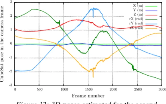
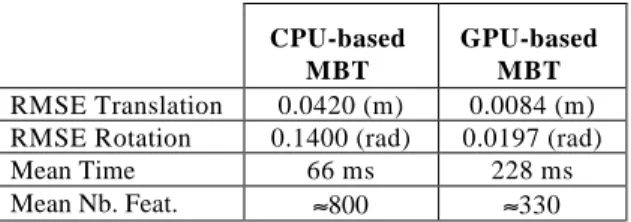
Regarding this second sequence, the CPU-based approach has not been able to correctly estimate the navigation data along the complete sequence (see Figure 12 and 13) while the GPU-based one has still been perfectly able to do it with an extremely good RMSE (0.0084 meters on the translation and 0.0197 radians on the rotation, see Table 2). By comparing Figures 13 and 15 with Figures 10.c and 11.c around frame 1700, we are still facing the same issue as in the previous experiment. Indeed, for these frames, the panels of the target are orthogonally aligned with the focal axis of the camera, which creates incertitude on the orientation of the target. Furthermore, the target appears small with a low visibility (see Figure 10.c). As a result, the CPU-based approach has not been robust enough to correctly estimate the navigation data around frame 1700 (see Figure 13). Hopefully, as soon as the CubeSat has reappeared in the image with better conditions, this issue disappeared and the CPU-based approach has been able to recover correct results.

Note that in the presented approaches, no detection method has been implemented in parallel to the tracking. However, we could benefit from such algorithms to recover the target pose when tracking fails as, for example, in [17, 18].

Figure 12: 3D poses estimated for the second sequence by using the CPU-based approach (translation in meters and rotation in radians).

Figure 13: Error to ground truth for the CPU-based approach on the second sequence.

Figure 14: 3D poses estimated for the second sequence by using the GPU-based approach (translation in meters and rotation in radians).

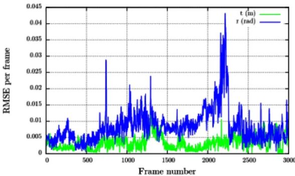
Figure 15: Error to ground truth for the GPU-based approach on the second sequence.

-3 -2 -1 0 1 2 3 0 500 1000 1500 2000 2500 3000 Cube Sat pos e i n the c ame ra frame Frame number X (m) Y (m) Z (m) rX (rad) rY (rad) rZ (rad) 0 0.1 0.2 0.3 0.4 0.5 0.6 0.7 0 500 1000 1500 2000 2500 3000 R MSE pe r fr ame Frame number t (m) r (rad) -3 -2 -1 0 1 2 3 0 500 1000 1500 2000 2500 3000 Cube Sat pos e i n the c ame ra frame Frame number X (m) Y (m) Z (m) rX (rad) rY (rad) rZ (rad) 0 0.1 0.2 0.3 0.4 0.5 0.6 0.7 0 500 1000 1500 2000 2500 3000 R MSE pe r fr ame Frame number t (m) r (rad)

4 CONCLUSION

In this paper, we have presented two model-based tracking approaches that have been developed and tested on various experiments with different conditions. While the first method (which is available in the ViSP framework [19]) is only relying on a CPU, the second one is also taking benefit of using a low-end GPU. Furthermore, in addition to the edge-based and keypoint-based features also used in the first approach, the second one is also considering color-based features (that could be adapted to intensity-based features if needed). This has aimed to increase the robustness of the navigation process in order to face with complex situations, as shown for the second image sequence.

While considering space applications, the graphics processing unit might not be available and the central processing unit might not be powerful enough to run complex algorithms. However, when dealing with damaged or complex objects (which will probably be the case in the future of the RemoveDEBRIS mission), or when dealing with hard environment conditions as presented in the second experiment, the CPU version might not be robust enough and could eventually fail to estimate the navigation data. In those cases, the GPU-based approach remains a better choice.

References

[1] N. W. Oumer, G. Panin, Q. Mülbauer, A. Tseneklidou, Visibased localization for on-orbit servicing of a partially cooperative satellite,

Acta Astronautica, 117:19-37, 2015.

[2] G. Bleser, Y. Pastarmov, and D. Stricker. Real-time 3d camera tracking for industrial augmented reality applications. Journal of WSCG, pp. 47–54, 2005.

[3] A.I. Comport, E. Marchand, M. Pressigout, and F. Chaumette. Realtime markerless tracking for augmented reality: the virtual visual servoing framework. IEEE T-VCG, 12(4):615–628, July 2006.

[4] T. Drummond and R. Cipolla. Real-time visual tracking of complex structures. IEEE PAMI, 24(7):932–946, July 2002.

[5] A. Petit, E. Marchand, and K. Kanani. Tracking complex targets for space rendezvous and debris removal applications. IEEE IROS’12, pp. 4483– 4488, Vilamoura, 2012.

[6] G. Panin, Al. Ladikos, and A. Knoll. An efficient and robust real-time contour tracking system.

IEEE ICVS, 2006.

[7] V. Prisacariu and I. Reid. Pwp3d: Real-time segmentation and tracking of 3d objects. British

Machine Vision Conf., September 2009.

[8] C. Bonnal, J.-M. Ruault, M.-C. Desjean, Active debris removal: Recent progress and current trends, Acta Astronautica, 85:51-60, April 2013. [9] J. Forshaw, G. Aglietti, N. Navarathinam, H.

Kadhem, T. Salmon, et al. An in-orbit active debris removal mission - REMOVEDEBRIS: Pre-Launch update. IAC'2015, Jerusalem, Oct. 2015. [10] A. Petit, E. Marchand, A. Kanani. Combining

complementary edge, point and color cues in model-based tracking for highly dynamic scenes.

IEEE Int. Conf. on Robotics and Automation, ICRA'14, pp. 4115-4120, Hong Kong, June 2014.

[11] R.T. Howard, A.S. Johnston, T.C. Bryan, M.L. Book, Advanced video guidance sensor (AVGS) development testing, Defense and Security, Int.

Soc. for Optics and Photonics, Orlando, 2004.

[12] P.-J. Huber, Robust Statistics. Wiley, New York, 1981.

[13] J. Shi and C. Tomasi, Good features to track, IEEE Int. Conf. on Computer Vision and

Pattern Recognition, CVPR '94, Seattle, 1994.

[14] M. Pressigout, E. Marchand. Real-time hybrid tracking using edge and texture information. Int.

Journal of Robotics Research, 26(7):689-713, July

2007.

[15] G. Panin, E. Roth, and A. Knoll. Robust contour-based object tracking integrating color and edge likelihoods. VMV 2008, pp. 227–234, Konstanz, 2008.

[16] E. Marchand, H. Uchiyama, F. Spindler. Pose estimation for augmented reality: a hands-on survey. IEEE T-VCG, 2016.

[17] A. Petit. Robust visual detection and tracking of complex object: applications to space autonomous rendez-vous and proximity operations. Ph.D.

thesis, Université de Rennes 1, December 2013.

[18] A. Petit, E. Marchand, R. Sekkal, K. Kanani. 3D object pose detection using foreground-background segmentation. IEEE Int. Conf. on

Robotics and Automation, ICRA'15, pp.

1858-1865, Seattle, May 2015.

[19] E. Marchand, F. Spindler, F. Chaumette. ViSP for visual servoing: a generic software platform with a wide class of robot control skills. IEEE Robotics

and Automation Magazine, 12(4): 40-52, 2005. CPU-based

MBT

GPU-based MBT

RMSE Translation 0.0420 (m) 0.0084 (m) RMSE Rotation 0.1400 (rad) 0.0197 (rad)

Mean Time 66 ms 228 ms

Mean Nb. Feat. ≈800 ≈330

Table 2: Second sequence: Root mean square errors (in meters for the translation and radians for the rotation), mean time and mean number of features per