Towards Soft Real-Time Applications on Enterprise Desktop Grids

HAL Id: inria-00000993

https://hal.inria.fr/inria-00000993

Submitted on 11 Jan 2006

HAL is a multi-disciplinary open access

archive for the deposit and dissemination of

sci-entific research documents, whether they are

pub-lished or not. The documents may come from

teaching and research institutions in France or

abroad, or from public or private research centers.

L’archive ouverte pluridisciplinaire HAL, est

destinée au dépôt et à la diffusion de documents

scientifiques de niveau recherche, publiés ou non,

émanant des établissements d’enseignement et de

recherche français ou étrangers, des laboratoires

publics ou privés.

Towards Soft Real-Time Applications on Enterprise

Desktop Grids

Derrick Kondo, Bruno Kindarji, Gilles Fedak, Franck Cappello

To cite this version:

Derrick Kondo, Bruno Kindarji, Gilles Fedak, Franck Cappello. Towards Soft Real-Time Applications

on Enterprise Desktop Grids. [Technical Report] 2005. �inria-00000993�

Towards Soft Real-Time Applications

on Enterprise Desktop Grids

Derrick Kondo, Bruno Kindarji, Gilles Fedak, and Franck Cappello

Bat 490, Universit´e Paris Sud, 91405 ORSAY Cedex, FRANCE Corresponding author: dkondo@gmail.com

Abstract— Desktop grids use the idle cycles of desktop PC’s

to provide huge computational power at low cost. However, because the underlying desktop computing resources are volatile, achieving performance guarantees such as task completion rate is difficult. We investigate the use of buffering to ensure task completion rates, which is essential for soft real-time applications. In particular, we develop a model of task completion rate as a function of buffer size. We instantiate this model using parameters derived from two enterprise desktop grid data sets, evaluate the model via trace-driven simulation, and show how this model can be used to ensure application task completion rates on enterprise desktop grid systems.

I. INTRODUCTION

For over a decade, the largest distributed computing plat-forms in the world have been desktop grids, which use the idle computing power and free storage of a large set of networked (and often shared) hosts to support large-scale applications. Desktop grids are an extremely attractive platform because there offer huge computational power at relatively low cost. Currently, many desktop grid projects, such as SETI@home [1], FOLDING@home [2], and EIN-STEIN@home [3], use TeraFlops of computing power of hundreds of thousands of desktop PC’s to execute large, high-throughput applications from a variety of scientific domains, including computational biology, astronomy, and physics.

Despite the huge return-on-investment that desktop grids offer, the platform’s use has been limited to mainly task parallel, high-throughput applications. This is a consequence of the resources’ volatility and heterogeneity. That is, the resources are volatile in the sense that CPU and host avail-ability fluctuates tremendously over time. This is because the hosts are shared with the owner/user, whose activity is given priority over the desktop grid application; at any time, an executing desktop grid task may be preempted due to user activity (e.g. key/mouse activity, other user processes, and etc.). Moreover, the hosts are heterogeneous in terms of clock rates, memory sizes, and disk sizes, for example. As a result of such volatility and heterogeneity, broadening the range of desktop grid applications is a challenging endeavor.

In this paper, we focus on enabling soft real-time ap-plications to execute on enterprise desktop grids; soft real-time applications often have a deadline associated with each task but can afford to miss some of these deadlines. While this problem entails a myriad of issues (such as timely data transfers), our goal is to achieve probabilistic guarantees on

task completion rates via buffering. That is, we determine how large a buffer must be allocate to ensure that some fraction of tasks meet their corresponding deadlines. We concentrate particularly on achieving such guarantees on desktop grids in enterprise environments, for example a company’s local area network. This is a challenging because task execution can be delayed or cancelled by users’ preemptive activity or machine hardware failures.

A number of soft real-time applications ranging from in-formation processing of sensor networks [4], real-time video encoding [5], to interactive scientific visualization [6], [7], [8] could potentially utilize desktop grids. An example of such an application that has soft real-time requirements is on-line parallel tomography [7]. Tomography is the construction of 3-D models from 2-3-D projections, and it is common in electron microscopy to use tomography to create 3-D images of bio-logical specimens. On-line parallel tomography applications are embarrassingly parallel as each 2-D projection can be decomposed into independent slices that must be distributed to a set of resources for processing. Each slice is on the order of kilobytes or megabytes in size, and there are typically hundreds or thousands of slices per projection, depending on the size of each projection. Ideally, the processing time of a single projection can be done while the user is acquiring the next image from the microscope, which typically takes several minutes [9]. As such, on-line parallel tomography could po-tentially be executed on desktop grids if there were effective method for meeting the application’s relatively stringent time demands.

To enable such soft real-time applications to utilize desktop grids, we investigate the use of buffering to ensure task completion rates. In particular, the contributions of this paper can be summarized as follows. First, we develop a model of the successful task completion rate as function of the server’s buffer size. Second, in the process of verifying the model’s assumptions, we show that the aggregate compute power of desktop grid systems can often be modelled using a normal distribution. Third, in the process of developing the model and running trace-driven simulations, we found several guidelines to be used when scheduling tasks with soft deadlines on volatile resources and describe them in detail.

The paper is structured as follows. In Section II, we formal-ize the specific problem that we address, describing in detail our application and platform model. Then, in Section III, we

characterize two desktop grid systems in an effort to instantiate parameters in our model using realistic values. In Section IV, we develop a model of task completion rate as function of buffer size. We describe in Section VI how our work in this paper relates to previous research. Finally, in Section VII, we summarize our conclusions and describe future research directions.

II. PROBLEMSTATEMENT

In this section, we formalize the problem that we address in this paper. In particular, we detail the application and platform model shown in Figure 1. Table I summarizes the variable definitions given in this section.

Fig. 1. Application and Platform Model

A reader periodically reads input data from disk into an input buffer (see Figure 1, step 1) of sizeb. We assume each input datum corresponds to a single task and use the term task synonymously with the term input datum. Specifically, the reader inserts a batch with H input tasks into the input buffer everyCintime units. Each task is assigned a deadlined, which denotes the maximum amount of time allowed to expire before the corresponding result becomes useless;d defines the soft real-time constraint of an application. The length of d is directly related to the length of the buffer and is given by

d = (b ∗ Cin)/H (1)

We assume the application can tolerate a small percentage of tasks that fail to complete by the deadline.

The total number of tasks isT . We assume the execution of each tasks is independent of one another, and that all tasks are of equal size s, which denotes the amount of computational work (in floating point operations for example) required to complete a task. For tasks with large input data sizes, we assume that the data transfer time can be folded in with the task

sizes. A clear limitation of our platform model it that does not

include a detailed and precise model of the network. Accurate network models is currently an open and difficult problem in parallel and distributed computing, and so, we postpone the inclusion of a more accurate network model for future work.

A scheduler is then responsible for scheduling a task from the input buffer to the set of N workers (see Figure 1, step 2). If a task’s deadline passes, or if the buffer overflows with too many tasks, the scheduler will delete tasks from the buffer. However, once a task is scheduled, the scheduler does not have the ability to cancel an executing task. (Although implementable, most desktop systems such as BOINC [10], XtremWeb [11], and Entropia [12] do not provide preemption mechanisms.)

Once assigned a task, a worker downloads the task from the scheduler (see Figure 1, step 3) and computes a result during its idle time. If the task fails (for example, because of user keyboard/mouse activity, or hardware failure), we assume the scheduler will detect the failure immediately and can then reassign the task. (Fast failure detection can be done through the use of worker heartbeats or time out mechanisms). Or if the task completes, the worker uploads the result to the scheduler, which then removes the task from the input buffer and places the result in the output buffer . Upon completion, a writer then writes the results in the output buffer to disk (see Figure 1, step 4).

The workers are heterogeneous, unreserved and shared machines. As such, they can have different processor speeds, and at any given moment in a time, an executing task can be preempted because of the desktop user’s activity. In particular, we denote the amount of computational power (in floating point operations, for example) usable by the

desktop grid application between time t and t + δ on

worker i as pt,t+δi where δ is some time interval and 1 ≤

i ≤ N . The value of pt,t+δi ranges between 0 and δ ∗

host’s maximum number of operations per second.

Several factors can influence the value of pt,t+δi . For in-stance, if the desktop machine i is powered off or there is continuous user keyboard activity between time t and t + δ,

then pt,t+δi would most likely be 0. If another process if

running on the machine, thenpt,t+δi may be some fraction of the maximum possible value. If pt,t+δi measures the compute power from an individual host, then the total amount of computational powerPt,t+δ_{available from the entire platform} consisting of N workers is given byPN_i=1pt,t+δi .

In our analysis based on previously described model, the performance metric we use is the percent of tasks that suc-cessfully complete before their corresponding deadlines, and we refer to this metric as the task success rate (or inversely, the task failure rate).

III. CHARACTERIZATION

Using the formulation described in the previous section, our goal is to construct a model to estimate the rate at which task deadlines are met as a function of the buffer size. To construct a such a model, one needs to first understand the characteristics of the platform’s aggregate compute power during some interval of time. The aggregate compute power is directly related to the rate at which tasks that can be completed.

Because desktop grid hosts are volatile, clearly some frac-tion of the aggregate compute power cannot be used as tasks begin to execute but then fail to run to completion. Thus, one also needs to characterize the volatility of the platform and in particular, the rate at which tasks fail to meet their deadlines. The rate at which tasks fail to meet their corresponding deadlines is also directly related the task success rate.

In this section, we give a statistical characterization of these two variables Pt,t+δ _{(the aggregate compute rate) and f}

dl (the rate at which a task does not complete by the deadline), and then use these variables in a model described later in Section IV.

A. Trace Data Sets

For both characterization and simulation purposes, we use the UC Berkeley (UCB) trace data set first described in [13]. The traces were collected using a daemon that logged CPU and keyboard/mouse activity every 2 seconds over a several weeks on about 85 hosts. The hosts were used by graduate students the EE/CS department at UC Berkeley. We use the largest continuously measured period between 2/28/94 and 3/13/94, and focus on the busiest periods of user activity between the hours of 10AM to 5PM. The traces were post-processed to reflect the availability of the hosts for a desktop grid application using the following desktop grid settings. A host was considered available for task execution if the CPU average over the past minute was less than 5%, and there had been no keyboard/mouse activity during that time. A recruitment period of 1 minute was used, i.e., a busy host was considered available 1 minute after the activity subsided. Task suspension was disabled; if a task had been running, it would immediately fail with the first indication of user activity.

The clock rates of hosts in the UCB platform were all identical, but of extremely slow speeds. In order to make the traces usable in our simulations experiments for modern-day applications, we transform clock rates of the hosts to a clock rate of 1.5GHz, which is a modest and reasonable value rela-tive to the clock rates found in the other current desktop grid platforms. Doing so, we assume that the effects of user CPU and mouse/keyboard activity has remained constant over the years. Several works, such as [14] and [15], provide evidence that many desktop grids characteristics have remained similar over time.

In addition to the UCB data set, we use another trace data set collected from desktops at the San Diego Supercomputer Center (SDSC), first reported in [14]. This data set was collected by submitting compute-intensive tasks to about 200 hosts at SDSC through the Entropia desktop grid system [12], which ensured that a task would only run when the machine was free. When permitted to execute by the Entropia desktop grid system, each task would continuously compute floating-point operations and log the number of operations completed every 10 seconds. The tasks’ output was then retrieved and used to create a continuous trace of CPU availability for each host. Because the tasks were executed through a real desktop grid system, the CPU availability perceived by the task is

exactly the performance that would be obtained by a real compute-intensive desktop grid application. Using the above method, traces for over 200 hosts with host speeds ranging 179MHz to 3.0GHz over a 1 month period were obtained.

B. Normality of Aggregate Compute Power

We hypothesize thatPt,t+δ _{can be modeled with a normal} distribution. Intuitively,Pt,t+δ _{is the sum of several random} variablespt,t+δi for1 ≤ i ≤ N . The central limit theorem [16] states that the sum of a set of variates from any distribution with a finite mean and variance tends towards a normal distribution. By the central limit theorem, for large relatively large i,Pt,t+δ _{should be distributed normally.}

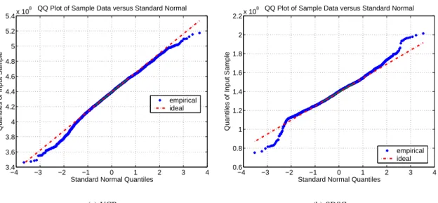
To test this hypothesis, we first measured Pt,t+δ _at thou-sands of different values oft and with δ equal to 60 second intervals. The rationale for using 60 second intervals is that task sizes would rarely be shorter than 60 seconds. We then conducted a parameter fit of this data set with a normal distribution using maximum likelihood estimation (MLE) [16]. MLE is a standard and the most popular technique for parameter estimation used for statistical modelling purposes. Intuitively, the MLE method finds parameter values for a particular distribution that maximize the probability that the data set came from that particular distribution. For the normal distribution, a MLE solver will attempt to maximize a likeli-hood function of µ and σ given the data set. After applying MLE to the data set, we found the estimate of the mean µˆ and standard deviationσ to be 4.3829 ∗ 10ˆ 8 _{and2.6136 ∗ 10}7 operations per second respectively for UCB trace data set. For the SDSC data set, the estimated mean µ and standardˆ deviation σ were 1.3998 ∗ 10ˆ 8 _{and 1.5630e + 07 operations} per second, respectively.

To measure the fit of the data set with respect to the normal probability distribution corresponding to the derived parameters, we conduct both a graphical test via a quantile-quantile (QQ) plot and a quantitative test via the Kolmogorov-Smirnov (KS) goodness-of-fit test. A QQ plot plots the quan-tiles of the empirical data versus the quanquan-tiles of the normal distribution. If the empirical data does in fact come from a normal distribution, the resulting plot will be linear (even if the empirical distribution is shifted or re-scaled relative to the normal distribution).

As depicted in Figures 2(a) and 2(b), we find that the QQ plots exhibits a strong linear relationship between the quantiles of the empirical and modelled distributions, and this in turn gives evidence thatPt,t+δ_{is distributed normally. The QQ plot} for the SDSC data set is slightly skewed at the ends compared to the ideal. Nevertheless, the cumulative distribution function (CDF) of the empirical data versus the fitted is virtually indistinguishable. After careful visual inspection of the SDSC traces, we suspect that the skew (which occurs with relatively very few data points) is due to a few “abnormal” events, such as coordinated backups of all the hosts which would reduce the CPU availability of all hosts simultaneously resulting in relatively low values ofPt,t+δ_.

−4 −3 −2 −1 0 1 2 3 4 3.4 3.6 3.8 4 4.2 4.4 4.6 4.8 5 5.2 5.4x 10 8

Standard Normal Quantiles

Quantiles of Input Sample

QQ Plot of Sample Data versus Standard Normal

empirical ideal (a) UCB −4 −3 −2 −1 0 1 2 3 4 0.6 0.8 1 1.2 1.4 1.6 1.8 2 2.2x 10 8

Standard Normal Quantiles

Quantiles of Input Sample

QQ Plot of Sample Data versus Standard Normal

empirical ideal

(b) SDSC Fig. 2. Quantile-quantile plot of empirical data for Pt,t+δ

In addition, to comparing graphically the empirical data set with the hypothesized normal distribution, we use the Kolmogorov-Smirnov (KS) test. Intuitively, the KS test reflects the maximum difference between the observed CDF of the data set and the expected CDF of the test distribution.

For large data sets (such as our empirical data set for

Pt,t+δ_{), the KS test is “too sensitive” in the sense that it}

will almost always reject the null hypothesis that the data follow the normal distribution as it detects very minor dif-ferences between the empirical data and the data from the hypothesized distribution. For large data sets gathered from real environments, a certain amount of noise will occur in the data sets and one cannot expect these data sets to match the hypothesized distribution perfectly.

So instead of using the KS test on the entire data set as a whole we use the a similar method deployed in [17] to de-termine whether the sample data could have the hypothesized distribution. That is, we conduct many KS tests on subsamples randomly selected from the entire data set. In particular, we conducted KS tests on 1000 subsamples of the data, each with about 100 randomly chosen data points, and then determine the mean p-value to either reject or accept the null hypothesis. We find that the resulting mean p-value of the KS tests with the UCB data to be 0.466, and the mean p-value of the KS test with the SDSC data to be .448, which are clearly above the traditional .05 threshold. While this should not be interpreted as absolute proof in support of the null hypothesis, it does provide additional quantitative evidence for the validity of our hypothesized distribution, which complements the results of our graphical tests.

The combination of our graphical test and KS test provide strong evidence thatPt,t+δ _{is distributed normally. So despite} the volatility of desktop grid resources, we find that certain ag-gregate statistics of the computational power of these resources can be modelled accurately with probability distributions.

The fact thatPt,t+δ _{follows a normal distribution is useful} for several reasons. First, one can accurately estimate the variance and determine confidence intervals for aggregate desktop grid performance. In past work [14], [13], [18], only the mean performance is presented and this point estimator does not reflect the volatility of the underlying system. This could have a number of important applications in multi-job scheduling (where the system is inundated with high-throughput and short-lived jobs, and the scheduler must give confidence intervals for throughput and response time), and also soft real-time applications that need guarantees on task completion rates. We give an example of the applying the normality result to the latter in the following section.

Second, when joining multiple desktop grids, it is possible to estimate the combined compute power easily. That is, given two desktop grids whose aggregate compute power

are P1t,t+δ and P

t,t+δ

2 with normal distributions N (µ, σ

2₎

and N (ν, τ2_{) respectively, then the combined desktop grid’s}

aggregate compute powerP1,2t,t+δ is distributed normally with expectationµ + ν and variance σ2

+ τ2

[16]. Obtaining such a statistic may be useful for estimating the cost and benefit (for example total compute power and reduction in variance) of joining two desktop grids infrastructures. The amalgamation of multiple desktop grids with different software infrastructures has been a topic of much past and present work [19], [20], [21] in the area of Grid computing.

C. Estimating deadline failure rates

Previously, we determined a method for modelling a desktop grid’s aggregate compute power. However, an application, especially one with large task sizes, may not utilize all of the aggregate compute power of the system because of task failures. That is, during execution on a host, a task may in fact be preempted by user CPU or keyboard/mouse activity, for example; in this case a small fraction of the aggregate

compute power is not used and application completion does not progress.

Thus, to determine the effective compute power of a desktop grid system for an application with a particular task size, one must first determine the rate at which tasks fail to meet their deadlines. We determine the steady state failure rate as follows. Using trace driven simulation, we execute a job with an infinite number of tasks over the entire trace period and then determine the number of tasks that complete before their deadline. We do this for a range of buffer sizes to determine the failure rate as a function of buffer size. (Note that if a task failed to complete on the host chosen first, we would randomly pick another host on which the task would be restarted from scratch, and we would repeat this process until the deadline expired or the task was finished.)

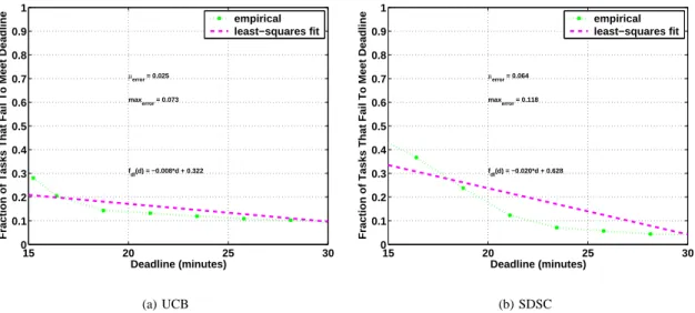
Figures 3(a) and 3(b) show the task failure rates on the UCB and SDSC platforms respectively for deadlines in the range of 15 and 35 minutes for a 15-minute task (that is, a task that takes 15 minutes to execute on a 1.5GHz machine). Clearly,

as d approaches infinity, the task failure rate will approach 0,

and sofdl(d) will decrease sublinearly. While the function is slight curved, we believe that the function can be estimated sufficiently by a linear function for a relatively small range of deadlines; in particular, we believe that a reasonable range of task success rates (which we discuss later in Section IV) of interest to system developers (e.g. ≥80%) corresponds to a range of deadlines in which fdl(d) appears almost linear.

So, we determined the least squares fit among the data points (also shown in Figures 3(a) and 3(b)), and determined the following linear relationships between deadline and failure rate for the UCB platform: fdl(d) = −0.008 ∗ d + 0.322

Since d = f (b) = (Cin/H) ∗ b,

fdl(f (b)) = (−0.008 ∗ Cin∗b)/H + 0.322 (2)

We found that for the UCB platform the mean and maximum error between the least-squares fit and simulation result to be 0.025 and 0.073 respectively.

For the SDSC platform, we found the following linear relationship between the failure rate and deadline: fdl(d) = −0.020 ∗ d + 0.628 with a mean and maximum error of 0.064 and 0.118 respectively. In a similar fashion, we determine the least-squares fit for applications with several other task sizes, and found fits with similarly small error values.

IV. MODELLINGTASKSUCCESSRATE

Previously, we determined that the aggregate compute power can be modelled by a normal random variable, and we determined a function describing the linear relationship between failure rate and task deadline. In this section, we show the usefulness of these statistics by applying them to help enable a soft real-time application to run on an enterprise desktop grid. In particular, we construct a model of the task success rate as function of those statistics and other parameters, in particular the buffer size. For convenience, Table I summarizes the parameters that we first introduced in Section II.

Parameter Definition

b Buffer size

H Tasks per batch

Cin Period by which a batch of tasks is inserted into the

input buffer

d Task deadline

s Task size

pt,t+δ_i Compute power available between time t and t + δ for worker i

Pt,t+δ _{Aggregate compute power available between time t}

and t + δ for the entire desktop grid

T Number of tasks in the application

N Number of workers in the platform

fdl Rate at which tasks fail to meet their deadline

S Fraction of tasks completed before their deadlines TABLE I

PARAMETERDEFINITIONS.

The minimum buffer size is a function of the desktop grid’s aggregate compute powerPt,t+δ _{and the rate at which tasks} enter the buffer and is given by:

b ≥ ((H ∗ s)/(Cin∗Pt,t+δ)) ∗ H

≥(H2

∗s)/(Cin∗Pt,t+δ)

(3) The reason for the secondH in equation 3 is to account for the fact that H tasks are added to the input queue at each periodCin. So we need to scale the buffer size accordingly.

Intuitively, the task success rate should be equal to the frequency thatPt,t+δ _{is above some threshold minus the task} failure rate given some deadline. To understand this, it is useful to consider each variable in isolation. Suppose that the resources are complete dedicated and so the deadline failure rate is 0. Then clearly the success rate is entirely dependent

on Pt,t+δ _{being above some threshold. Now suppose that}

Pt,t+δ _{is very large relatively to the number and frequency}

of incoming tasks. Then clearly, the task success rate depends on the rate at which tasks can run to completion before the deadline.

More formally, the task success rate as a function of the buffer size can be given by:

S(b) = P r(Pt,t+δ _{> α) − f}

dl(f (b))

where α is some constant and fdl(f (b)) can be estimated by the results of Section III-C.

Moreover, using equation 3, we derive the following:

P r(Pt,t+δ _{> α) = P r(P}t,t+δ _≥(H2

∗s)/(Cin∗b)).

Then, for the UCB platform, the task success rate as a function of buffer size is given by:

S(b) = P r(Pt,t+δ_{> (H}2

∗s)/(Cin∗b))−

((−0.008 ∗ Cin∗b)/H + 0.322)

(4) The intuition behind the above equation is that tasks can fail to meet their deadlines for two reasons. Firstly, failure can occur if the aggregate compute power in the system dips below the incoming work rate. The probability that this occur is given by

P r(Pt,t+δ _{> (H}2_∗s)/(C

in∗b)). Secondly, failure can occur if

15 20 25 30 0 0.1 0.2 0.3 0.4 0.5 0.6 0.7 0.8 0.9 1 fdl(d) = −0.008*d + 0.322 µerror = 0.025 maxerror = 0.073 Deadline (minutes)

Fraction of Tasks That Fail To Meet Deadline

empirical least−squares fit (a) UCB 15 20 25 30 0 0.1 0.2 0.3 0.4 0.5 0.6 0.7 0.8 0.9 1 fdl(d) = −0.020*d + 0.628 µerror = 0.064 maxerror = 0.118 Deadline (minutes)

Fraction of Tasks That Fail To Meet Deadline

empirical least−squares fit

(b) SDSC Fig. 3. Fraction of 15-minute tasks that fail to meet deadline.

if the aggregate compute power in the system is always greater than the incoming work rate, i.e.,P r(Pt,t+δ_{> (H}2

∗s)/(Cin∗

b)) = 1, host unavailability may still cause some tasks to fail in meeting their deadlines. This is particularly relevant to the UCB platform, where the intervals of availability tend to be quite small. (This is a consequence of the relatively strict criteria for which a host is considered available, i.e., the host cannot have any other user processes running, any keyboard/mouse activity is disallowed, and etc.)

We plot the success rate S(b) as a function of the buffer size, represented by the solid blue line in Figures 4(a), 4(b), and 4(c) for 65 ≤ b ≤ 130, which correspond to applications with 5-minute, 15-minute, and 25-minute tasks respectively. We set the number of tasks per batchH to be 64, which is large enough so that any host that was available always received a task so that the entire computing power of the platform would be utilized. We choose a minimum value of 65 for b since clearly b must be greater than or equal to H. Initially, for relatively small buffer sizes, S(b) is relatively low, but as b increases S(b) dramatically increases until a buffer size of 70, at which point the curve’s “knee” occurs. Thereafter,S(b) increases at a much lesser rate. For example, for an application with 15-minute tasks shown in Figure 4(b), a buffer size of 70 results in a .80 success rate, where as a buffer size of 120 only results in a 10% increase in success rate.

The shape of the curve can be explained as follows. For relatively small buffer size values, i.e., between 65-70, the success rate value is dominated by P r(Pt,t+δ _{≥ (H}2

∗

s)/(Cin∗b)); Pt,t+δ is normally distributed with a relatively

small variance, and so small changes inb dramatically affect

P r(Pt,t+δ _≥(H2

∗s)/(Cin∗b)). Moreover, because we set

the batch size H so that the entire system is saturated with tasks,P r(Pt,t+δ _≥(H2

∗s)/(Cin∗b)) dramatically changes

for values of b close to H. For buffer sizes greater than 70,

P r(Pt,t+δ_≥(H2

∗s)/(Cin∗b)) becomes close to one, and so

the success rate is dominated more by the deadline failure rate,

which explains the more gradual increase in success rate with an increase withb. The above explanation applies similarly to the results for the SDSC platform shown in Figures 5(a), 5(b), and 5(c). We chose a slightly different range for the buffer size in these plots as the least-squares fit for fdl was more accurate in this smaller range; specifically, we used the result in Figure 3(b) to determine a range of interest (asfdl gives a lower bound on the success rate), and then “bootstrapped” by determining thefdl in that new smaller range.

V. MODELAPPLICABILITY

One potential weakness in our model is that the steady-state failure ratefdlwas measured using a job with an infinite number of tasks. We were concerned thatfdlwould in fact be too pessimistic because tasks submitted in the previous batches would interfere with the progress of tasks in the most recently submitted batch. That is,fdlcould be too pessimistic if tasks of previous batches that failed to complete immediately would remain in the queue (until their deadline passed) and thus delay the execution of tasks of the current batch such that these tasks would “starve” and miss their deadlines. In turn, this might affect the applicability of the model for jobs with a relatively small number of batches.

To determine the accuracy offdland the result of including it in our model, we determined the mean success rate for an application with a relatively small number of batches (10). (This represents a worst-case scenario, i.e., increasing the number of batches would only improve our model’s accuracy.) To do this, we ran trace-driven simulations of the execution of jobs with 5, 15 and 25-minute tasks and 10 batches.

We chose thousands of different starting points in the traces to begin a job and executed the job via trace-driven simulation. The red dotted line in Figures 4 and 5 shows the mean result of running these simulation experiments for various buffer sizes on the UCB and SDSC platforms, respectively. Also shown in those figures are the critical mean (µcr

70 80 90 100 110 120 130 0 0.2 0.4 0.6 0.8 1 Buffer size

Task success rate

µcr error = 0.005

maxcr_error = 0.013

model result simulated result

(a) 5 min. tasks

70 80 90 100 110 120 130 0 0.2 0.4 0.6 0.8 1 Buffer size

Task success rate

µcr error = 0.018 maxcr_error = 0.032 model result simulated result (b) 15 min. tasks 70 80 90 100 110 120 130 0 0.2 0.4 0.6 0.8 1 Buffer size

Task success rate

µcr error = 0.029 maxcr_error = 0.062 model result simulated result (c) 25 min. tasks Fig. 4. Task success rate versus buffer size on UCB platform.

80 90 100 110 120 130 0 0.2 0.4 0.6 0.8 1 Buffer size

Task success rate

µcr error = 0.030 maxcr error = 0.063 model result simulated result

(a) 5 min. tasks

80 90 100 110 120 130 0 0.2 0.4 0.6 0.8 1 Buffer size

Task success rate

µcr error = 0.030 maxcr_error = 0.055 model result simulated result (b) 15 min. tasks 80 90 100 110 120 130 0 0.2 0.4 0.6 0.8 1 Buffer size

Task success rate

µcr error = 0.031 maxcr_error = 0.064 model result simulated result (c) 25 min. tasks Fig. 5. Task success rate versus buffer size on SDSC platform.

(maxcr

err) between the model and simulation results; we define

µcr

err and maxcrerr to be the mean and maximum errors for range in whichS(b) is greater than .80 because we believe that system developers will not be concerned as much with success rates below this threshold. We found that the maximum error between the model and simulation results to be .063 over both platforms’ results, which indicates a precise fit between the model and simulated results.

The close fit between the model and simulation results can be explained by the way in which tasks are scheduled to hosts. Firstly, tasks are dropped from the buffer if there is no host on which the task can completed before its deadline. Virtually all desktop grid systems [22], [10], [11], [12] keep track host clock rate information, and so it is reasonably to assume that a scheduler can determine whether a host can complete a task by the deadline if it were completely dedicated to task execution. We found that this trivial policy resulted in significant (>10%) improvement in terms of task success rates. Secondly, tasks are dropped in First-In-First-Out (FIFO) order so that if the buffer ever overflows as incoming tasks are placed in the queue, then the oldest tasks are removed from the queue first. For these

reasons, the negative affect of old tasks starving newly arrived ones is greatly reduced.

Ironically, what we believed was a weakness in the way we calculatedfdl was its strength. Becausefdlmeasures the rate at which tasks fail to meet their deadlines when the system

is in steady state, fdl takes into account the effect that older

tasks have on the execution newly arrived ones. Alternatively, we had first erroneously measured fdl by just using random incidence. In particular, we chose hundreds and thousands of starting points for a task on each host over the entire trace period, and determined whether the task could be completed by a particular deadline, assuming the platform was entirely

free. This resulted in a failure rate that was inaccurate by 10%

precisely because it did not consider the fact that other tasks already in the system could prevent newly arrived tasks from completing by their deadlines. While an error of 10% may seem negligible in absolute terms, if the curves in Figures 5 and 4 had been shifted down by 10%, the corresponding buffer sizes would have changed dramatically (and would therefore be not as accurate).

as a result,S(b) tends to be a lower bound on the true success rate. This explains why the S(b) is slightly lower than the simulation results shown in Figures 4 and 5;

To apply the plots shown in Figures 4 and Figure 5, a desktop grid developer could use the graph to determine what buffer size is needed to achieve some desired success rate. For example, suppose an application consists of 15-minute tasks. Using Figure 4(b), if a 90% success rate for the application is acceptable, then a buffer size of about 120 would be needed, and the developer can then determine the amount of RAM necessary to make the success rate achievable. Conversely, if a desktop grid server already has some amount of memory, then a desktop grid developer could determine the corresponding buffer size and task success rate that will be result by such a configuration. Another way to use the result is determine the cost effectiveness of add more memory to a server. For example, if the server’s current memory size can support a maximum buffer size of 65 tasks, it may be worthwhile to purchase slightly more memory to support a maximum buffer size of 70 tasks, thereby increasing the success rate by 20%. In contrast, if 120 tasks can already be stored in the server’s memory, purchasing the same amount of memory to increase the number of buffered tasks to 125 will only improve the success rate by less than 3%.

VI. RELATEDWORK

There is related work in several different areas, namely desktop grid characterization, performance modelling, and scheduling for soft real-time applications. With respect to characterization, several papers [18], [14], [23] report the mean aggregate compute power of desktop grid systems, but do not detail the distribution. The work in [14] also reports failure rates, but the definition of failure rates is entirely different from that as defined in this paper. In [14], a failure is defined to be a task execution that fails run to completion. In this paper, a failure is a task that is not completed by a specific deadline; so although a task execution may fail to run to completion, the task may still successfully complete in time on a different host. As discussed in Section IV, using the latter definition of failure is essential for our model’s accuracy. In [17], the authors use similar (and standard) statistical modelling techniques on desktop grid data sets. However, they model availability intervals, i.e., the time elapsed between two consecutive machine failures. In contrast, in Section III-B, we model the aggregate compute power of each desktop grid within some time period, which is entirely different from availability intervals, and thus arrive at different conclusions regarding its distribution.

In [24], [17], the authors give evidence that machine availability follows Weibull or hyperexponential distributions. While their models could potentially be incorporated into our model to determine task failure rates, we opted to take an empirical approach to model task failure rates as it was unclear whether the same probability distributions reported in [17] could model availability in our desktop grid traces. Moreover, the trace data sets used in that study were not available, so if

we used the identical probabilistic model described in [17] to determine task failure rates, it would be difficult to verify our new model’s accuracy.

Also, there has been much work in the area of performance modelling and scheduling on desktop grids [25], [26], [27], [28], [29], [30], [31]. To the best of our knowledge, none of these works use an application model where the goal is to determine the affect of buffer size on task completion rates with respect to a deadline. In addition, there has been some work on scheduling soft real-time applications on non-dedicated systems [6]. However, in these systems, the def-inition of CPU availability is quite different. That is, user activity (e.g. keyboard/mouse activity, or user processes) does not necessarily preempt a running desktop grid task; instead, the machines are shared between the desktop grid task and other users. As a result, the resources modelled in that study are much less volatile than those used here.

VII. SUMMARY ANDFUTUREWORK

We described a closed-form model for task success rate as a function of buffer size. Our model assumed that the aggregate compute power of a desktop grid can be modelled as a normal probability distribution, and we showed the validity of our assumption via traces derived from two real desktop grid systems. Moreover, our model used the task deadline failure rate as a parameter, and we showed that such failure rates can be modelled adequately with a least-squares fit. Our model can be used by system developers who wish to determine an adequate buffer size for their (soft real-time) application to guarantee a certain task completion rate.

For future work, we plan on looking at replication tech-niques as an alternative means of improving the task success rate. Replication invariably “wastes” resources as they com-pute redundant tasks, and as such, it is only option when there are more hosts relative to the number of tasks. We hope to extend our current model to predict task success rate as a function of replication levels.

ACKNOWLEDGMENTS

We gratefully acknowledge Kyung Ryu and Amin Vahdat for providing the UCB trace data set and documentation.

REFERENCES

[1] W. T. Sullivan, D. Werthimer, S. Bowyer, J. Cobb, G. Gedye, and D. Anderson, “A new major SETI project based on Project Serendip data and 100,000 personal computers,” in Proc. of the Fifth Intl. Conf. on Bioastronomy, 1997.

[2] M. Shirts and V. Pande, “Screen Savers of the World, Unite!” Science, vol. 290, pp. 1903–1904, 2000.

[3] “EINSTEN@home,” http://einstein.phys.uwm.edu.

[4] “Sensor Networks,” http://www.sensornetworks.net.au/network.html. [5] A. Rodriguez, A. Gonzalez, and M. P. Malumbres, “Performance

evaluation of parallel mpeg-4 video coding algorithms on clusters of workstations,” International Conference on Parallel Computing in Electrical Engineering (PARELEC’04), pp. 354–357.

[6] J. Lopez, M. Aeschlimann, P. Dinda, L. Kallivokas, B. Lowekamp, and D. O’Hallaron, “Preliminary report on the design of a framework for distributed visualization,” in Proceedings of the International Conference on Parallel and Distributed Processing Techniques and Applications (PDPTA’99), Las Vegas, NV, June 1999, pp. 1833–1839.

[7] S. Smallen, H. Casanova, and F. Berman, “Tunable On-line Parallel Tomography,” in Proceedings of SuperComputing’01, Denver, Colorado, Nov. 2001.

[8] I. Foster and C. Kesselman, Eds., The Grid, Blueprint for a New Computing Infrastructure, 2nd ed. Morgan Kaufmann, 2003, ch. Chap-ter 8: Medical Data Federation: The Biomedical Informatics Research Network.

[9] A. Hsu, Personal communication, March 2005.

[10] T. B. O. I. for Network Computing, http://boinc.berkeley.edu/. [11] G. Fedak, C. Germain, V. N’eri, and F. Cappello, “XtremWeb: A Generic

Global Computing System,” in Proceedings of the IEEE International Symposium on Cluster Computing and the Grid (CCGRID’01), May 2001.

[12] A. Chien, B. Calder, S. Elbert, and K. Bhatia, “Entropia: Architecture and Performance of an Enterprise Desktop Grid System,” Journal of Parallel and Distributed Computing, vol. 63, pp. 597–610, 2003. [13] R. Arpaci, A. Dusseau, A. Vahdat, L. Liu, T. Anderson, and D. Patterson,

“The Interaction of Parallel and Sequential Workloads on a Network of Workstations,” in Proceedings of SIGMETRICS’95, May 1995, pp. 267– 278.

[14] D. Kondo, M. Taufer, C. Brooks, H. Casanova, and A. Chien, “Char-acterizing and Evaluating Desktop Grids: An Empirical Study,” in Proceedings of the International Parallel and Distributed Processing Symposium (IPDPS’04), April 2004.

[15] K. D. Ryu, “Exploiting idle cycles in networks of workstations,” Ph.D. dissertation, 2001.

[16] R. Larsen and M. Marx, An Introduction to Mathematical Statistics and its Applications. Prentice Hall, 2000.

[17] D. Nurmi, J. Brevik, and R. Wolski, “Modeling Machine Availability in Enterprise and Wide-area Distributed Computing Environments ,” Dept. of Computer Science and Engineering, University of California at Santa Barbara, Tech. Rep. CS2003-28, 2003.

[18] A. Acharya, G. Edjlali, and J. Saltz, “The Utility of Exploiting Idle Workstations for Parallel Computation,” in Proceedings of the 1997 ACM SIGMETRICS International Conference on Measurement and Modeling of Computer Systems, 1997, pp. 225–234.

[19] N. Andrade, W. Cirne, F. Brasileiro, and P. Roisenberg, “OurGrid: An Approach to Easily Assemble Grids with Equitable Resource Sharing,” in Proceedings of the 9th Workshop on Job Scheduling Strategies for Parallel Processing, June 2003.

[20] O. Lodygensky, G. Fedak, V. Neri, F. Cappello, D. Thain, and M. Livny, “XtremWeb and Condor: Sharing Resources Between Internet Con-nected Condor Pool,” in Proceedings of the IEEE International Sym-posium on Cluster Computing and the Grid (CCGRID’03) Workshop on Global Computing on Personal Devices, May 2003.

[21] H. Casanova, G. Obertelli, F. Berman, and R. Wolski, “The AppLeS Parameter Sweep Template: User-Level Middleware for the Grid,” in Proceedings of SuperComputing 2000 (SC’00), Nov. 2000.

[22] M. Litzkow, M. Livny, and M. Mutka, “Condor - A Hunter of Idle Workstations,” in Proceedings of the 8th International Conference of Distributed Computing Systems (ICDCS), 1988.

[23] W. Bolosky, J. Douceur, D. Ely, and M. Theimer, “Feasibility of a Serverless Distributed file System Deployed on an Existing Set of Desktop PCs,” in Proceedings of SIGMETRICS, 2000.

[24] M. Mutka and M. Livny, “The available capacity of a privately owned workstation environment ,” Performance Evaluation, vol. 4, no. 12, July 1991.

[25] L. Gong, X. Sun, and E. Waston, “Performance Modeling and Prediction of Non-Dedicated Network Computing, Tech. Rep. 9, 2002.

[26] X. Sun and M. Wu, “Grid Harvest Service: A System for Long-Term, Application-Level Task Scheduling,” in Proceedings of the International Parallel and Distributed Processing Symposium (IPDPS’03), April 2003. [27] M. Adler, Y. Gong, and A. Rosenberg, “Optimal sharing of bags of tasks in heterogeneous clusters,” in Proceedings of the Fifteenth Annual ACM symposium on Parallel Algorithms and Architectures, San Diego, California, 2003.

[28] Y. Li and M. Mascagni, “Improving performance via computational replication on a large-scale computational grid,” in Proc. of the IEEE International Symposium on Cluster Computing and the Grid (CC-Grid’03), May 2003.

[29] S. Leutenegger and X. Sun, “Distributed Computing Feasibility in a Non-Dedicated Homogeneous Distributed System,” in Proc. of SC’93, Portland, Oregon, 1993.

[30] G. Ghare and L. Leutenegger, “Improving Speedup and Response Times by Replicating Parallel Programs on a SNOW,” in Proceedings of the 10th Workshop on Job Scheduling Strategies for Parallel Processing, June 2004.

[31] S. Bhatt, C. F., F. Leighton, and A. Rosenberg, “An Optimal Strategies for Cycle-Stealing in Networks of Workstations,” IEEE Trans. Comput-ers, vol. 46, no. 5, pp. 545–557, 1997.