A survey of graph and subgraph isomorphism problems

(1)

Université de Montréal

A survey

of

Vo5

graph and subgraph isomorphism problems

par

Yaohui Lei

Département d’informatique et de recherche opérationnelle Faculté des arts et des sciences

Mémoire présenté à la Faculté des études supérieures en vue de l’obtention du grade de

Maîtrise ès sciences (M.Sc.) en informatique

Avril. 2003

(2)

)ûQL

f î

(3)

Université

dl1

de Montréal

Direction des bibliothèques

AVIS

L’auteur a autorisé l’Université de Montréal à reproduire et diffuser, en totalité ou en partie, par quelque moyen que ce soit et sur quelque support que ce soit, et exclusivement à des fins non lucratives d’enseignement et de

recherche, des copies de ce mémoire ou de cette thèse.

L’auteur et les coauteurs le cas échéant conservent la propriété du droit

d’auteur et des droits moraux qui protègent ce document. Ni la thèse ou le mémoire, ni des extraits substantiels de ce document, ne doivent être

imprimés ou autrement reproduits sans l’autorisation de l’auteur.

Afin de se conformer à la Loi canadienne sur la protection des renseignements personnels, quelques formulaires secondaires, coordonnées

ou signatures intégrées au texte ont pu être enlevés de ce document. Bien

que cela ait pu affecter la pagination, il n’y a aucun contenu manquant.

NOTICE

The author of this thesis or dissertation has granted a nonexclusive license

allowing Université de Montréal to reproduce and publish the document, in part or in whole, and in any format, solely for noncommercial educational and

research purposes.

The author and co-authors if applicable retain copyright ownership and moral

rights in this document. Neither the whole thesis or dissertation, nor substantial extracts from it, may be printed or otherwise reproduced without the author’s permission.

In compliance with the Canadian Privacy Act some supporting forms, contact

information or signatures may have been removed from the document. While this may affect the document page count, it does not represent any loss of

(4)

Université de Montréal

Faculté des études supérieures

Ce mémoire intitulé:

A survey

0f

graph and subgrapb isomorphism problems

présenté par:

Yaohui Lei

a été évalué par un jury composé des personnes suivantes:

Alain Tapp (président-rapporteur) Cilles Brassard (directeur de recherche) Gena Hahn (Co-directeur de recherche)

Pierre McKenzie (membre de jury)

(5)

Abstract

Graphs are useful as a flexible and versatile data structure for the representation of objects and concepts. _{The graph and subgraph isomorphism problems have been thoroughly} studied for decades. _{They have been drawing great interest in many theoretical and} practical domains including transport planning, chemistry, geographv, information retrieval, automata theory, linguistics, computer-aided-design, mathematics and computer science. An introduction and prelirninaries begin this surve. This includes basic computational cornplexity theory, group theory and grapli theory. Then, we begin the graph isomorphisrn by showing the isomorphism-complete class. Some special graph isomorphisms in the P class are presented from two approaches: combinatorial approach and group-theoretic approach.

The survey is followed hy an analysis of the suhgraph isomorphism problem. First, we give an overview of complexity resuits for this problem. Then, we present some special subgraph isornorphisms such as subtree, planar suhgraph. etc.

from the practical algorithms point of view, several graph and subgraph isomorphisrn algorithms are introduced. A performance comparison of these algorithms is outlined.

At. the end of the survev, w’e give n conclusion and a discussion of these problems. Since

we usually refer to special cases for these problems, we consider some other possibilities which might be interesting.

Key words: graph isomorphism, subgraph isomorphism, computational complexity, group theory, isomorphism-complete class, combinatorial approach, group-theoretic approach

(6)

Résumé

Les graphes sont utiles comme une structure de données flexible et versatile pour la représentation des objets et des concepts. Les problèmes de l’isomorphisme de graphe et l’isomorphisme de sous-graphe ont été bien étudiés depuis des décennies. Ils ont été pris du grand intérêt dans beaucoup de domaines théoriques et pratiques incluant la planification de transport, chimie, géographie, recherche d’information, automates théorie, linguistique, Conception Assistée par ordinateur, des mathématiques et informatique.

Une introduction et les préliminaires commencent cette synthèse. Ceci inclut la base de la théorie de complexité du calcul, la théorie de groupe et la théorie de graphe. Ensuite. nous commençons l’isomorphisme de graphe en montrant la classe isomorphisme-complet. Quelques isomorphisms spéciaux de graphe dans la classe de P sont présentés de deux approches : approche combinatoire et approche groupe-théorétique.

La synthèse est suivie d’une analyse du problème d’isomorphisme de sous-graphe. D’abord. nous donnons une vue générale des résultats de complexité pour ce problème. Puis, nous présentons certains isomorphisms spéciaux de graphe tels que le arbre, le sous-graphe planaire, etc.

Du point de vue d’algorithmes pratiques, plusieurs algorithmes sur l’isomorphisme de graphe et l’isomorphisme de sous-graphes sont présentés. Une comparaison de performance de ces algorithmes est décrite.

À

la fin de cette synthèse, nous donnons une conclusion et une discussion de ces problèmes. Puisque nous référons souvant à des cast spéciaux pour ces problèmes, nous considérons quelques autres possibilités qui pourraient être intéressantes.

Mots-clés: isomorphisme de graphe, isomorphisme de sous-graphe, complexité du calcul, théorie de groupe, isomorphisme-complet, approche combinatoire, approche groupe-théorique

(7)

C

5 Conclusion and Discussion ₁₀₀ 5.1 Review 100 5.1.1 On graph isomorphisrn ₁₀₀ 5.1.2 On subgraph isornorphism ₁₀₁ 5.1.3 On practical algorithms ₁₀₁ 5.2 Look ahead ₁₀₂

5.2.1 Turn to other graplis ₁₀₂

5.2.2 Probabilistic vs. deterministic ₁₀₃

5.2.3 Quantum vs. classical ₁₀₄

5.3 A propos de t.his survey 107

(11)

List of Figures

1.1 two examples of isomorphic graphs ₃

1.2 sample computation tree of an ATM 9

1.3 classes P and NP ₁₄

2.1 change a graph to a bipartite graph 28

2.2 a chordal graph 29

2.3 reduction of graph G, G and Ç 31

2.4 self-complementary graphs 33

2.5 self-complementary digraph ₃₄

3.1 an example of subtree isomorphism ₇₃

3.2 decision tree representation 85

3.3 reduction of the decision tree to BDD 86

(12)

List of Algorithms

1 find the minimal tree distance decomposition 55

2 check if G and H are isomorphic 56

3 ISO_CHECK procedure ₅₇

4 GETIB sub-procedure ₅₉

5 subtree-Isornorphism(G H) ₇₄

6 LI’vIDFS on two embedded graphs ₈₁

7 embedded subgraph isomorphism 82

8 Nauty algorithm ₉₂

(13)

Chapter 1 Introduction and Preliminaries

1.1 Introduction

Graphs are useful as a flexible and versatile data structure for the representation of objects ancl coiicepts. It is well known that graph representations are widely used for dealing with structural information in different domains such as transportation, networks, image

interpretation and processing, computer-aided design, pattern recognition, and many other subflelds of science and engineering. For example, the intersections and traffic routes of a city can be represented by graphs. The intersections are represented b vertices whule the routes are drawn as edges in a graph.

Two graphs are equat if they have the same vertex set and the same edge set. But there are other ways in which two graphs could be regarded as being the same. For instance, one could regard two graphs as being “the same” if it is possible to rename the vertices of one and obtain the other. Such graphs are identical in everv respect except for the names of the vertices. In this case, we cali t.he graphs isomorphic. When graphs are small enough,

(14)

CHAPTER 1. INTRODUCTION AND PRELIMIIVARIES 2

whether two graphs are isomorphic can he detect.ed easily rnanually, whule this becomes

infeasible when the graphs are rnuch bigger.

In this survey, we give an overview of the subject not only from a theoretical point of view but also from a practical aspect. On the one hand, we give an introduction and preliminaries to the mathematics in order to make understanding casier. On the other hand. cornplicated proofs and algorithms with deep theorv background are simplified and outlined. Nevertheless, in order to keep tue integrity and the continuity, some of these

proofs and algorithms are quoted alrnost verbatim from t.heir sources.

1.1.1 Graph isomorphism

The graph isomorphism (GI) problem was listed as an important open problem already in Karp

_[•51

over three decades ago. The graph isomorphism problem is deciding whether two given graphs are isomorphic, i.e. whether there is a bijective mapping from the vertices of one graph to the vertices of the second graph such that the edges are respected. Much work

1791

is dedicated to the search for an exact isomorphism between two graphs or subgraphs.

IL is a problem of interest in many theoretical and practical domains

₁₇₉₁

including transport planning, chemistrv, geography, information retrieval, automata theory, linguistics, computer aided-design, mathernatics and computer science 123, 30.

891.

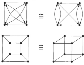
Graphs represent various real structures or situations: we want to know whether two structures or situations are essentiallv the same with respect to a selected point of view, in other words, isomorphic.

f igure 1.1 gives two examples: one is for the directed graph and the other is for the

undirected graph.

The GI problem is very simple to define and understand, but it seems very difficuit to give an efficient solution, i.e. a polynoinial-time algorithm. Because of its theoretical and

(15)

CHAPTER 1. INTRODUCTION AND PRELIMINARIES 3

practical importance the problem has been studied from many different points of view

[511. There are some algorithms to solve this problem, but they have an exponential time complexity [79]. Hence, time complexity is the main issue of the graph isomorphism problem.

1.1.2 Subgraph isomorphism

While graph isornorphism treats _{the isomorphism relation between whole graphs, the} subgraph isomorphism _{focuses on subgraphs of one graph. Subgraph isomorphism problem}

is to determine whether there is a subgraph of one given graph which is isomorphic to

a given second graph. Subgraph isomorphism is very important in computer vision, bio-computing and image processing. Like graph isomorphism, it has been studied in depth for hoth theoretical and practical interests. _{For example, t1271. one of possible} applications of suhgraph isomorphism is for finding whether a given chemical compound is a sub-compound of a further specified compound, given the structural formulas. Moreover, subgraph isomorphism is an important and very general form of exact pattern matching, such as string searching, sequence alignment, tree comparison and pattern matching on

(16)

CHÀPTER 1. INTRODUCTION AND PRELIMINARIES 4

graphs.

$ubgraph isomorphism is a common generalization of many important graph prohiems f47], including Hamilton paths, cliques, matchings, girth, and shortest paths. Most of the research on subgraph isomorphism algorithms bas been based either on heuristic search techniques as in f35, 127], or on constraint satisfaction techniques as in [40, 931• The best known algorithms for subgraph isomorphisrn are based on a relational view approach [40] on exhaustive search with backtracki;ig.

The rest of this survey is organized as follows. Chapter 1 introduces the terminology and preliminaries on computational complexity, group theory and graph theory. Chapter 2 focuses on the graph isomorphism problem. Complexity resuits, combinatorial and group theoretic approaches to solve graph isornorphism problem are shown as well as polynomial time algorithrns on special cases of graphs such as trees, planar graphs, bounded valence graphs, etc. In Chapter 3, the subgraph isomorphism prohiem is discussed by presenting complexitv resuits in subtrees, planar graphs and embedded graphs. Another point of view regarding subgraph isomorphism, the relational view, is presenteci too. As for practical algorithms in graph and subgraph isomorphism problems, Chapter 4 shows basic ideas of major algorithms, Nauty, Ullmann and $chmidt & Druffel, along with a comparison of performance. A conclusion and a discussion of these aspects are given in Chapter 5.

1.2 Basic computational complexity

In this section, we give a brief overview of computational complexity theory. For more detailed description, readers are encouraged to consult [3, 110, 1111.

(17)

The theorv of computation, a subfield of computer science and mathematics, is the studv of mathematical models of computing, independent of any particular computer hardware. Complexity theory is part of the theory of computation dealillg with the resources required during computation to solve a given problem. The most common resources are tirne (how many steps it takes to solve a problem) and space (how much memory it takes to solve a problem).

Given a problem. we need an algorithm to solve it. How do we know that an algorithm is a “good” one? À useful measure of performance is “the time or space required to solve a problem as a function of the size of data”. Generally speaking, computational complexity theory studies:

• the efficiency of algorithms

• the inherent difficultv of problems of practical and/or theoretical importance

An important cliscovery in the area is that computational problems can vary tremendously in the effort required to solve them precisely.

Definition J Considerfunctions

_f,

g: N - R. Say that f(n) is ofthe order ofg(n), written f(n)

e

O(g(n)) (catted big-O notation), if tÏzere is a positive constant c such that for every n, f(n) < c g(n).

Algorithms which have a polynomial or sub-polynomial time complexity (that is, they take time f(n)

e

O(g(n)), where g(n) is a polynomial), are often practical.

Algorithms with complexities which cannot be bounded by polynomial functions are called exponential-time algorithms.

(18)

CHÀPTER 1. INTRODUCTION ÀND PRELIA’IINARIES ₆

1.2.1 Turing machine

In computational complexity theory, we use frequently the idea of a Turing machine. A Turing machine is an abstract model of computer execution and storage introduced in 1936 by Alan Turing to give a mathematically precise definition of “algorithm” or “mechanical proceclure”.

Definition 1.2 A Turing machine consists of:

1. A tape which is divided into ceïts, one next to the other. Each ceïï contains a symbol

from some finite alphabet. The alphabet contains a speciaï bïank symbot and one or more other symboïs. The tape is assumed to be arbitrariïy extendible to the ïeft and to the right, i.e., the Turing machine is aïways suppïied with as much tape as it needs for its computation. Ceïïs that have not been written to during a computation are

assumed to be fiïïed with the bïank symbot.

2. A head that can read and wTite symboïs on the tape and moue ïeft and right.

3. A state register that stores the state of the Turing machine. The number of different

states is aïways finite and there is one special start state with which the state register is initiaïized. Some states may be designated as “accept” states.

4.

A transition table that teïïs the machine what symbol to write, how to moue the head

(“L”for one step left, and “R”for one step right) and what its new state will be, given the symbol it has just read on the tape and the state it is currently in. If there is no entry in the table for the current combination of symbol and state then the machine wiïl haït.

(19)

CHAPTER 1. INTRODUCTION AND PRELIMINARIES f

5. The Turing machine accepts its input if it halÉs in an “accept” state and refuses

otherwise.

Definition 1.3 _{An ordinary (deterministic) Turing machine (DTM,) is a triple:}

T (Q,Z,F.6,qo,B.f)

where

_Q

_{is a fuite set of states, F is the finite set of tape symbots, B}

_e

_{F is the blank} symbot, Z C _{F is the set of input symbots, 6 :}

_Q

_x _F —*

Q

x f x {L, R} is the moue fanction,

qo

e Q

is the start state and f C

_Q

_{is tÏie set of final states.}

Definition 1.4 An non-deterministic Turing machine (NTM,) is a triple:

T =

(Q,

Z, F, 6,qo, qaccept, qreject)

where

_Q

_{is a fuite set of states, Z is the input alphabet, not containing bÏank symbot, F is} the fuite set of tape symbots, 6 :

_Q

x f —*

Q

x f x {L, R} is the moue function, q0 _E

_Q

_is

the start state, Qaccept E

Q

is the accept state and qreject

e Q

is the reject state.

A NT1\’I differs from a DTM in that rather than a single instruction triplet, the transition rulemay_{specifv a number of alternate instructions. NTM cari be thought of a generalization} of DTM. At each step of the computation we can imagine that the computer “branches” into rnany _{copies, each of which executes one of the possible instructions. Whereas a DTM} has a single “computation path” that it follows, a NTM has a “computation tree”. If any branch of the tree haits with an “accept” condition, we say that the NTM accepts the input.

(20)

• nu is the current tape contents;

• n is the part (possibty empty) of the string frorn the Ïeftrnost symboÏ titi the scanned

ceÏt of the tape;

• if a is the symnbot in the scanned ccii, then u is the part (possibiy empty) of the string

from a to rightrnost non-biank syrnboÏ.

• q is the current state.

We next. define Alternating Turing Machine (ATM). Just as an NTM is a generalization of a DTM, an ATM is a generalization of an NIM.

Definition 1.6 An ATM M

_(Q,

,F, ,F)

(Q

is a set of states, F is the tape alphabet, 6 is the transition function, _{is the input alphabet, and F is the set of final states) is an}

NTM with the foïlowing differences:

1. Each state q E

Q

is a pair < n, z >. where z

e

{“Universat”, “Existentiat”} is a “label” for the state and n is the state narne. This partitions

_Q

into a set of existentiat

₎

_{states and a set of universal (V) states. Fix an input x.} _{We cati} a configuration (tape contents, position of R/W head, state of controt,.) to be an existentiai configuration if its state is existential. Univers al configurations are deflned sirnilarly.

2. Acceptance of M: If a Turing Machine can legally go from a configuration C1 to

another configuration C2 in a single step according to the transition function, C1 is catted the parent of C2 or C2 is the child of C1. Configurations without any children are caÏled leaf configurations and others are called non-teaf configurations. We now recursivety label each configuration to be either accepting or rejecting as follows.

(21)

CHÂPTER 1. INTRODUCTION AND PRELIMINARIES 9

(a) _{A teaf configuration whose state is a finat state is tabeted “accepting”. A teaf} configuration whose state is not a final state is labeted “rejecting’

(b) A non-teaf existentiat configuration is tabeÏed “accepting” if at teast one of its chiÏdren is ÏabeÏed “accepting’ and it is ÏabeÏed ‘rejecting”, otherwise. A non teaf uniue’rsat configuration is Ïabeted “accepti’ng” if alt of its chitdren are tabeted “accepting”, and it is Ïabeled “rejecting”, othermise.

(c) The M is said to accept the input x, if and onÏy if its starting configuration is tabeted “accepting”.

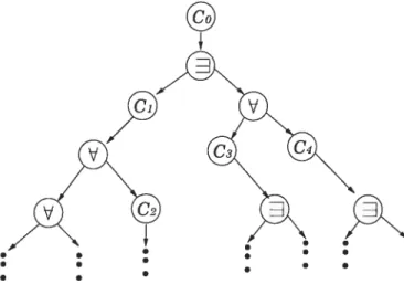
In thinking about the computation of an ATM, it is helpfui to represent the computation as a tree, see figure 1.2.

figure 1.2: sample computation tree ofan ATM

Each node of the tree is labeled with the machine’s configuration and has arrows pointing to the configurations reachable by outgoing transitions from the node. The outcome of the computation is determined redursively as follows. A node which is in the machine’s accept state qj accepts. A node in the state accepts if and only if at least one of its chiidren accepts. A node in the V state accepts if and only if both of its chiidren accept. Every

.

(22)

CHAPTER 1. II\’TRODUCTION AND PRELIMINARIES 10

other node has oniy one child, and accepts if arid only if its child accepts. The machine accepts if and only if the root of its computation tree accepts.

1.2.2 Decision problems

In the theory of computation a problem is a set of finite-length questions (strings) with associated finite-length answers (strings) .A decision problem is a problem that requires a YES or NO answer. Tiiese problems are also referred to as recogriition problems.

A decision problem is usually formalized as the problem of deciding whether a given string heiongs to some specified set of strings, also called a formai language. The set contains exactly those questions w’hose answers were “YE$”. If there is an algorithm that is a.hle to correctly decide for every possible input string whether it belongs to the language, then the problem is called decidabte and otherwise it is called ‘a’ndecidabÏe. Important points are

• If a problem is decidable, there is a Turing machine M that when processing any

instance, ï, of P (i.e., any string x on its input tape) will eventually finish in state

Qûcept ifï is a “YES” instance of the problem and will eventually finish in state _Qreject

if s is a “NO’ instance of the problem.

• A problem for which no such Turing machine exists is undecidable.

• Decision problems are a whole lot easier to deal with when looking for special

problems, like unsolvable problems. because proposed solutions only either accept or reject their input rather than producing some likely complex output on its tape that needs to be analyzed.

(23)

+

If we can find a decision problem that is undecidable, the we know that there are unsolvable problems. We don’t need to look for some very complex general problem that is unsolvable if we can find a very simple decision problem that we can prove is undecidable by showing that there is no possible Turirig machine that could decide it.

Computer programs, from a tiny “Hello, world!” procedure to a huge operating system. may be viewed as computing functions. Since all computers employ hinary notation. sucS functions are defined over sets of binarv strings. In considering the question “What problems can be solved by computers?”, it is sufficient to concentrate on decision prohiems. Hence, “What problems can 5e solved by computers?” is equivalent to “What decision problems can 5e solved?”.

Any binarv string can be viewed as a representation of some natural number. Thus for decision problems on binary strings we can concentrate on the set of functions of the form

f

: N {O, 1}

INPUT: n a natural number

OUTPUT: 1 ifn satisfies a given property; O ifn does not satisfy it.

An example is the Prime problem: return 1 if n is a prime number; O if n is a composite numher.

Decision problems are important because any general problem with an n-hit answer can he transformed into a decision problem with a YES/NO answer. $olving the general problem can’t 5e more than n times harder than solving the decision problem. There are several ways to do this transform. For example, if the general problem is of the form:

(24)

CHAPTER 1. INTRODUCTION AND PRELIMINA RIES 12

Given an input X, return the answer string Y

then the associated decision problem is:

Given an input X and an integer k, return whether the kth bit of Y is 1

1.2.3 Polynomial reductions and transformations

The basic tools for relating the complexities of various problems are polynomial reductions and transformations. We say that a problem A reduces to another problem B in polynomial time, denoted as A cxp B if:

1. there is an algorithrn for A which uses a subroutine for B, and 2. each cail to the subroutine for B counts as a single step, and 3. the algorithm for A runs in polynomial-time.

If A cx B and B x A we say that the problems are polynomially equivalent and write

The practical implication cornes frorn the following proposition and its contrapositive:

If A polynornially reduces to B and there is a polynomial-time algorithm for B, then there is a polynomial-time algorithm for A.

(25)

C’HAPTER 1. INTRODUCTION AND PRELIMINARIES 13

1. (A reduces to B) and (B is “easy”) ,‘ A is “easy”

2. (A reduces to B) and (A is “hard”) ,‘ B is “hard”

3. (A reduces to B) and (B is “hard”) == no conclusion for A - (a very common case)

4. (A reduces to B) and (A is “easy”) no conclusion for B - (also a very common

case)

That is. if A polynomiallv reduces to B. then B is at least as hard as A.

1.2.4 The classes P, NP, NP-hard and NP-complete

Definition 1.7 The cÏass P (polynomiat-time) consists of alt those decision pro btems that eau be sotved on a deteri inistic Taring machine in an amount of time tha.t is potynomiat in the size of the input; the cÏass NP (non-deterministic poÏynomzat-time) corisists of ail those decision probtems uhose positive solutions eau be verifled in polynomial time given

the right information, or equivatentty, whose solution con be found in polynomial time by a ‘non-determznzstzc Taring machine.

Definition 1.8 The NP-hard (Non-deterministic Potynomiat-time hard,) refers to the ctass of decision pro btems that contains alt probtems H such that for alt decision probtems L in NP there is a potynomiat-time many-one reduction to H. Informatly this ctass eau be described as coritaining the decision probtems that are at teast as hard as any pro blems in NP, atthough it might, in fact, be harder.

Definition 1.9 The NP-comptete is the comptexity ctass of decision probtems for which ans’wers can be checked for correctness by an aigorithm whose mn time is polynomial in the

(26)

CHÀPTER 1. INTRODUCTION ÀND PRELIMINARIES 14

size of the input (that is, it is NP) _{and no other NP probtem is more than a polynomial}

factor harder. InformaÏty, a probtem is NP-comptete if answers can be verified qnickty, and a quick atgorithm to soïve this probtem can be used to soïve alt other NP probtems quickÏy.

In complexity theory, the NP-complete problems are the hardest problems in NP, in the sense that they are the ones most likely flot. to be in P.

Clearlv. P C NP. Is P a proper subset of ATp? This is the most important open question in theoretical computer science. Most people think that the answer is probably “ves”. then there are some problems in NP which are not in P ($ee Figure 1.3).

If P = NP then ail of the NP probiems coHapse to P. Ladner [80] shows that this is the

only case.

Theorem 1.1 1fF NP then there exists sets in NP that are neither in P nor NP — compt etc.

Some people believe the question may be undecidable within the current axiornatization. A $1,000,000 prize [131] has been offered for a correct soliltion.

The question “Is P = NP ?“ can be rephrased as: if positive solutions to a YE$/NO problem can be verifled quickly, can the answers also be computed quickly? Here is an

(27)

example to get a feeling for the question. Given two large numbers X and Y, we might

ask whether Y is a multiple of some integer between 1 and X, exclusive. For example, we might ask whether 69799 is a multiple of some integer between 1 and 250. The answer is YES, though it would take a fair amount of work to find it manually. On the other hand, if someone daims that the answer is YES because 223 is a divisor of 69799, then we cari quickÏy check that with a single division. Verifying that a number is a divisor is much easier than finding the divisor in the first place. The information needed to verify a positive answer is often called a “certificate”. So we conclude that given the right certificates. positive answers to our problem can be verified quickly (i.e. in polynomial time) and that’s why this problem is in NP. It is not known whether the problem is in P. 11w special case where X — Y was first shown to he in P in 2002 11, after rnany years of

research.

The NP-cornplete term for hard problems essentially means: “abandon ail hope of finding an efficient algorithm for the exact solution of this problem”. We should point out that proving or knowing tha.t a problem is NP-complete is not all that negative. IKnowing such limitations, people do not waste time on impossible projects and instead turn to less ambitions approaches, for example to find approximate solutions, to solve special cases or to alter problems a httle so that they become tractable (even at a loss of some fit to real-life situation, which is particularly useful in practical application since sometimes we cannot provide or guarantee an exact mapping between “real life” and theoreticai representation). The goal of this theory is therefore to assist algorithm designers in directing their efforts toward promising areas and avoid impossible tasks.

A NP-complete problem has the following most important property. Finding an efficient algorithm for any NP-compÏete problem implies that an efficient algorithm can be found for all such problems, since any problem belonging to this class can be recast as any other

(28)

CHÀPTER 1. INTRODUCTION AND PRELIMINÂRIES 16

member of the class: they are ail polynomially equivalent.

The practical significance of showing the recognition version of an optimization problem to 5e NP-complete is that one should not pursue the search for a good optimizing algorithm for such a problem and 5e content with finding a good approximating (i.e. heuristic) algorithm.

1.2.5 The class NC

The class NC (short for “Nick’s Class”, introduceci by Nick Pippenger) is the set of decision problems decidable in polvlogarithmic time on a parallel computer with a polynomial number of processors. In other words, a problem is in NC if tliere are constants c and k such that it can 5e solved in time O((logn)c) using O(nk) _{parallel processors.}

Just as the class P can he thought of as the class of tractable problems, NC can be thought of as the class of prohiems that can 5e solvecl efficientlv on a parallel computer. It is unknown whether NC = P. but most researchers suspect this to lie false. meaning that

there are some tractable prohiems which are “inherentiy sequential” and cannot significantlv 5e sped up by using parallelism.

The parallel computer in the definition can 5e assurned to 5e a parallel, random-access machine (PRAM). That is, a parallel computer with a central 1)001 of memorv. and any processor can access any hit of memory in constant time.

1.3 Group theory preliminaries

We begin with a brief review of elementary facts from group theory, which we give usuallv without proofs. For details, readers eau consuit [6, 81]. It is essential to understanding the

(29)

recent approach, group-theoretic techniques, to solve graph isomorphism.

1.3.1 Group deftnitions

Definition 1.10 A group is a set G together with a binary operation o on G snch that

1. a o (b o c) = (o o b) o e, for alt a. b. c e G (associative Ïaw,

2. There exists an etement e E G, catted the identity eÏement, such that aoe eoa = a,

for alt a E G,

3. To each a E G, there exists an etement b, catÏed the inverse of a, such that a o b =

boa = e.

In the third condition, b is usuallv denoted as a hecause it is unique. For any e such

thataoc=coa=e,wehavec=coe=co(aob)=(coa)ob=b.

A common group example is = ({1, 2,.. ,p—l},

.),

where pis a prime and the operation

is multiplication modulo p.

The order of the group G is the number of its elernents and is denoted G. A group of order p’, with p a prime number and n> 1, is called a p-group.

Let G be a group and a E G. Let n be the smallest positive integer, if it exists, such that

e. Then n is called the order of a and we shah write order(a) = n. Que also says that a is of finite order with order n.

An element g E G such that order(g) = G is called generator. À group G that has such

(30)

CHÂPTER 1. INTRODUCTION AND PRELIMINÂRIES 18

À trivial group I is the group consisting of the identity e oniv.

À group G is commutative, if, for ail g, h E G, g o h h o _{g. Otherwise, G is non}

commutative. À commutative group is also called Abelian in honour of one of the first group theorists, Neils Henrik Àbel.

À nonempty subset H of a group G is called a subgroup of G if

1. a,b

e

H hnplies that ab E H,

2. e E H (where e is the identity of G),

3. a

e

H implies that a

e

H.

We write H < _{G, when H is a subgroup of G.}

À group G is calied permutation group if G is a set of permutations of a fixed set X and the group operation is the composition of permutations (wc think of a permutation as a bijection from the set X onto itself).

Let G1 and G2 5e groups with operations o, * respectively. The Cartesian prodiict

G1 x G2 is the set of pairs G1 x G2 = {(g1, ₉₂₎ g1

e

G1, g E G2}. Let us define a group

operation multiplication on G1 x G2. For two arbitrary elements (ai, a2) and (b1, b2) in

G1 xG2, define their product by (a1, a2)(b1, b2) = (aiobi, a2*b2). The set of ail ordered pairs

(.r1.x2) such that x1 E G1, and 12 E G2 form a group under the operation multiplication. We cail this group the direct product of G1 and G2.

Let X be a fixed set of cardinalitv n. Let Sym(X) denote the set of ail bijections from X onto it.self, i.e. the set of ail permutations of X, and let the operation be composition. Then Syrn(X) is a permutation group and is cailed the symmetric group on X. If Y

(31)

CHÀPTER 1. INTRODUCTION AND PRELIMINÂRIES 19

is another set of cardinalit n, then a bijective map

_f

between X a.nd Y defines a unique correspondence between the elements in Sym(X) and the elements in Sym(Y). This correspondence says that we have f(n) o f(ço) = f(ir o

)

for ail 7C, E $ym(X). We cali

f

an isomorphism between $ym(X) and $ym(Y). We usually choose X = {1, 2, ,

the set of the first n _{natural numbers. In this case, Sym(X) is abbreviated by S.}

A transposition is a permutation of a set. which fixes ail but two eiement.s. Let X he a set of cardinality greater than 1. Consider the set of those elements in Sym(X) which can be expressed as the product of an even number of transpositions. This set is cÏosed uncler composition and thus forms a permutation group Att(X) which is cailed alternating group on X. The order of Sym(X) is exactiy twice the order ofAit(X).

1.3.2 Cosets and Lagrange’s Theorem

Given H. a subgroup of G, and g E G, the set Hg = {h o g h E H} is a right coset of

H in G. Simiiarlv, the set gH = {g o h h E H} is a left coset of H in G. Note that H

is hoth a left anti a right coset of itself. It is easy to show that two left (right) cosets of H are either disjoint or equal, and that ail cosets are of cardinality equai to the order to H. Thus, we may partition G into the ieft (right) cosets of H.

The number of distinct left (equivalently. right) cosets of H is called the index of H in G, and is written [G : H].

Theorem 1.2 (Lagrange) The order of G is equat to the product of the order of H and the index of H in G, i.e. G = H X [G: H].

(32)

6HAPTER 1. INTRODUCTION ÀND PRELIMINARIES 20

1.3.3 The Orbit-$tabilizer Theorem

Definition 1.11 A group

G

is said to act on a set X when there is a rnap G x X — X such that the fottowing conditions hotd for alt etements x X:

• (e,

)

x where e is the icÏentity etement of G.

• (g, (h, x)) (gh. r) for alt g, h E G.

We write gx for x). Suppose that the group G acts on the set. X. If we start with the elernent ï

e

X and apply group element.s in ail possible wavs, we get

3(r) = {gï: g E G}

which is called the orbit ofï under the action of G. The action of G on X is transitive

(we also say that G acts transitively on X) if there is oniy one orbit, in other words, for any ï,y E X, there exists g E G such that gx y. Note that the orbits partition X, because they are the equivalence classes of the equivalence relation given by y ï if and

only if y = gx for some g

e

G.

The stabilizer of an element ï E X is

G(ï)={gEG:gx=ï},

the set of elements that leave ï fixeci. A direct verification shows that G(x) is a subgroup.

This is a useful observation because any set that appears as a stabilizer in a group action

(33)

CHAPTER 1. INTRODUCTION ÂND PRELIMINARIES 21

The following theorem, known as the Orbit-Stabilizer theorem, is fundamentai in many applications.

Theorem 1.3 Suppose that a group G acts on a set X. Let 3(x) be the orbit of x

e

X, and let G(x) be the stabitizer ofx. Then the size of the orbit is the index of the stabitizer, that is.

[G: G(x)].

Thus if G is fuite, then B(x) G/G(x); in particutar, the orbit size divides the order

of the group. D

1.3.4 Normal Subgroups, Homomorphism and Automorphism

A subgroup H of G is normal written H <

G,

if, for ail g

e G,

Hg = gH.

Let G and G’ 5e two groups, h a rnap from G to G’. Then the map h is a group homomorphism if, for all 91,92

e

G,

h(g1 •92) = h(g1) h(g2).

The set K of ail elements in G which are mapped to the identity e’ of G’ is a normal subgroup of G and is called the kernet of the homomorphism, denoted by Ker(h). If the subgroup K is I, the trivial group, then h is an isomorphism. The image of a homomorphism h is the set of ail the elements of G’ to which are mapped the elements of G, denoted by Im(h).

(34)

1.4 Graph prelimillaries

1.4.1 Basic graph terminology

Siiice graphs have been widely studied in different contexts, there are various different terminologies in this field. The comprehensive book written by Brandstiidt, Le and Sprinrad

_[251

is a good reference. The notation and concepts in this survev are hased on this hook.

+

A graph is an ordered pair of sets G = (V, E) where V (or 17(G) to emphasize that

it belongs to the graph G) is the vertex set and E (or E(G) to emphasize that it belongs to the graph G), E C {{n,v} n v,n E Vu E V}, the edge set. Usually,

the number ofvertices. tV is denoted bu n. while the number ofedges, lEI, is denoted bv rn. If e = {u, v} é E(G). we sav that vertices n and u are adjacent in G, and

that e joins n and y. We’ll also sa that n and u are the ends of e, denoted bu n E e,y E e. The edge e is said to be incident with n (and u

_),

and vice-versa. We

write nv (or un) to denote the edge {n,u}, on the understanding that no order is implied. Note that E(G) is a set. This means that twro vertices either are adjacent or are not adjacent, there is no possibility of more than one edge joining a pair of vertices. The elements of E are 2-subsets of V. Thus, a vertex cannot he adjacent to itself.

+

A digraph (short for directed graph) is an ordered pair of sets G ₌ (V, A), where

V is a set of vertices and A is a set of ordered pairs (called arcs) of vertices of V.

+

The open neighbourhood of a vertex u in a graph G is the set N(u) = {n nu E E};

(35)

CHAPTER 1. INTRODUCTION ÂND PRELIMINARIES 23

• The adjacency matrix of a graph on the vertex set {1,. ,n} is an nXn O-1 matrix

A = (ajj) in which the entr ajj = 1 if there is an edge from vertex i to vertex

j

and

is O if there is no edge between vertex i and vertex

j.

• The incidence matrix of a graph on the vertex set {1,. , n} and the edge set

{

... ,rn} is an n x ni matrix A (ajj) in which then entry = 1 if edge

j

is

incident with vertex j and O otherwise.

• A walk (or. e0—Cn walk) in a graph is an alternating sequence of vertices and edges.

e0, e1, e1. e2, e2, e3,e3.• ,e,1, e such that e = e4e for Ï < i < n. The integer n

is the length of the walk. It is the number of edges in the walk, one Ïess than the number of vertices. A closed walk is a walk that starts and ends at the same vertex.

• A trail is a waik in which no edge is repeated. $imilariy, a closed trail is a trail that

starts and ends at the same vertex. A path is a walk in whicli no vertex is repeated. A graph which lias a path between everv pair of vertices is cailed connected graph.

• A cycle (or circuit) is a closed path which does not contain a vertex twice (except

at the beginning and end).

• A loop is an edge that connects a vertex to itself.

• The distance dG(x,y) _{in graph G oftwo vertices x,y is the length} ofasliortest r—y path in G; if no such path exists. we set d(x, y) := oc.

• The greatest distance hetween anv two vertices in grapli G is the diameter of G,

denoted by diam(G).

• A wheel is a graph that consists of a cycle and one vertex in the “middle” whicli is

connected to ail the vertices on the cycle. An odd wheel is a wheei whose outer cycle is of odd iength, and an even wheel lias an even cycle for the “rim”.

(36)

• The girth of a graph G is the length of the shortest circuit of G (or infinity if G lias

no circuit).

• A tree is a connected graph that has no circuits. Sometimes it is convenient to consider one vertex of a tree as special; such a vertex is then called root of this tree. A tree with a fixed root is a rooted tree. Choosing a root r in a tree T imposes a. partial ordering on V(T) by letting x < _{y if (x, y)} _{T. This is the tree-order on} V(T) associated with T and r. Note r is the least element in this partial order, every leaf x r of T is a maximal element.

• The path P7 (n the number of vertices) is a tree witli two vertices of degree 1 and

the other (n — 2) vertices of degree 2. This graph is cailed path graph P.

• The subgraph of G induced by a subset W of its vertex set V (i.e. W V) is the graph formed by the vertices in W and ah the edges of G whose two endpoints are in W. It is del1oted as G[W]. Analogouslv, we define the suhgraph G[F] induced by the set of edges f.

• The complement

Ô

of G is a grapli on , but two distinct vertices are adjacent in

Ô

if and oniy if they are non-adjacent in G.

• A stable set of G is a subset of vertices with no edge between any two of them.

• The degree of a vertex V of G is the number of edges incident to it. It is also cailed

valence, is clenoted hy d(v) and is given hy d(v) — N(v).

• The connected components of a graph G are the connected subgraphs of G induced

by sets of vertices such that no two vertices in different sets are connected.

• A cut vertex is a vertex wliose rernoval (along witli ail edges incident with it)

(37)

• A complete graph is a graph in which any two distinct vertices are adjacent. A

complete graph on n vertices is denoted by K,. A clique of G is a complete subgraph ofG.

• The une graph L(G) of a graph G = (V, E) is the graph whose vertex set is E and

whose edge set is E’, where e1e2

e

E’ if and only if e1 and e2 are incident to the same vertex in G.

• A graph G is k-vertex-connected (resp. k-edge-connected) if we need to delete

at least k vertices (resp. k edges) in order to get a non-connected graph. The (vertex or edge)_connectivity of the graph is the largest k such that G is k-connected.

1.4.2 Graph homomorphism and isomorphism

Although we have mentioned several isornorphisrn terrns above, we would like to give the definitions formally since our approaches, presented later, frequently refer to them.

Definition 1.12 If G arid H are graphs, a kornornorphismfrom G to H is a rnap

f:

V(G) —* V(H)

with the property that f(n) is adjacent to f(v) whenever n is adjacent to u. A bijective homomorphism whose inverse is aÏso a horno’morphism is an isomorphisrn.

We writ.e G1 G if G1 and G2 are isomorphic.

Definition 1.13 An automorphism of a graph G is an isomorphism

_f

that rnaps G to itsetf. FormatÏy, an antomorphisrn ofa graph G is a one-to-one, onto map

_f

: V(G) —+ V(G)

(38)

Chapter 2 Graph Isomorphism

The GI problem has been intensively studied. It occupies an important position in the complexity family because no one knows what is its computational complexity. It is well known that. GI is in NP, but despite decades of study by mathematicians and computer scientists, it is flot known whether GI is in P or flot

f51J.

There is some evidence that it is not likely to be NP-complete [90, 126j. Many researchers conjecture that GUs complexity lies somewhere between P and NP-complete. If P L _{NP then, hy Ladner’s theorem [$0],}

there exist problems which are of intermediate status; many people think that GI lies in this level.

One earlv resuit on the complexitv of GI is an O(exp(nl/2+0(’))) _{(rnoderately exponential)} algorithrn due to Babai [9j. Moderately exponential means that on a problem of size n, the measure of computation, ïn(n), is more than any polynomial k _{but less than any} exponential c, where k > _{0, e> 1. Formally, m(n) is of moderately exponential growth if} for ail k> 0, m(n) Q(k) and for ail f > O , m(n) = o((1 + f)’).

The best existing upper hound for the problem is exp(cn logn) (c is a constant) given 26

(39)

HAPTER 2. GRAPH ISOMORPHISi’I ₂₇

by Luks and Zemlyachenko

_1141,

_{but there is no evidence of this bound being optimal.} By imposing certain restrictions on the properties of the graphs, however, it is possible to design algorithms that have polynomially bounded complexity. In the following sections, we vill give the cornplexity classes of restricted graph isomorphisrn problems which have been compiled hy many mathematicians during the last decades.

2.1 Isomorphism-complete class

The graph isomorphisrn problem is not isolated. It is, in fact, a class of problems. A rigorous discussion of the structural complexit of the graph isomorphisrn problem is given in Kdbler, Schôning, and Torân

_1781.

In an attempt to classify the graph isomorphism problem a new class of problems has been developed: the isomorphism-complete class

t591•

A prohiem is said to be isomorphism-complete if it is provably equivalent to the

isomorphisrn prohiem. This class includes problems that can he shown to he polnomially equivaleiit to the graph isomorphism problem.

As mentioned, the complexity of GI is polynomial if we add some restriction on the graphs. Conversely, many other restricted isomorphism problems are known to be polynomially equivalent to GI. It has been proved that the following types of graphs are in the isomorphism complete class: bipartite graphs, line graphs [63], rooted acyclic digraphs, chordal graphs, traiisitively orientable graphs, regular graphs

_[231,

_{directed path graphs [15], k-trees (unbounded} k), and comparability graphs [103]. In 1978, Colbourn

_[31

proved that the question of deciding whether a graph is self-complementary, is graph isomorphism complete. In 2002, Kaibel and Schwartz

(73]

proved that the problem of deciding whether two (convex) polytopes are combinatoriallv isomorphic is graph isomorphism-complete, even for simple or simplicial polytopes. In the same year, Nagoya, Uehara and Toda [1031 showed that

(40)

HÀPTER 2. GRÀPH ISOIVIORPHISM 28

chordal bipartite graphs are in the isomorphism-complete class, too.

Now we review several types of graphs in the isomorphism-complete class and give brief pro ofs.

2.1.1 Bipartite graph isomorphism

A bipartite graph is a graph G whose vertex set V can he partitioned into two non emptv sets Vj and in such a way that every edge of G joins a vertex in to a vertex in . An alternative way of thinking about it is as about colouring the vertices in V1 one colour and those in V2 another colour, with no edge between vertices of the same colour.

Theorem 2.1 Blpartite graph isomorphism graph zsorno7phzsrn.

Proof. Testing the isomorphism of bipartite graphs is isomorphism-complete. since any graph can he made bipartite bv replacing each edge by two edges connect.ed with a new vertex (see f igure 2.1).

a\/b

a

figure 2.1: change a graph to a bipartite graph

(41)

CHAPTER 2. GRAPH ISOAIORPHISM 29

2.1.2 Chordal graph isomorphism

Definition 2.1 [58] An undirected graph is catted chordat if every cycle of tength greater

than 3 possesses a chord, that is, an edge joining two nonconsecutive vertices of the cycle.

An example of chordal graphs is shown in figure 2.2. Chordal graphs are also called triangutated graphs, rigid-circuit graphs, monotone transitive graphs and perfect etimination graphs in the literature

[25].

Theorem 2.2 (Lueker and Booth [87J, 1979) Chordat graph isomorphism graph isomorphism.

Proof. We construct a polynomial mapping M from a graph G to a graph M(G) such that M(G) is a chordal graph, and G can be recovered from M(G) up to isomorphism. We will show that the question of whether G1 is isornorphic to G2 is reduced to the question of whether M(G1) is isomorphic to M(G2).

‘for the reduction to chordal graph isomorphism, let 11.1(G) =

G’

= (V’, E’), where V’ =

VUE. and

Figure 2.2: a chordal graph

(42)

CHAP TER 2. GRÀPH ISOMORPHISM 30

The construction can be implemented to t.ake O(n + in) time, where n V, in

Now, we consider any cycle of length greater that 3 in G’. If the cycle contains oniy V

vertices, then it lias a chord, since ail V-vertices are adjacent. Otherwise, the cycle contains an E-vertex, and then the two vertices adjacent to this E-vertex must be V-vertices, thus, they are adjacent. Therefore, G’ is chordai.

“Assume now that n 4. It turns out that G’ contains enough structure to aliow us to

reconstruct G, up to isomorphism. As a mat.ter of fact, since ail V-vertices are adjacent, ail of them have cÏegree at ieast equal to n — 1, which is more than 2, while E-vertices aiways

have degree 2, because an E-vertex is adjacent to exactly two V-vertices. Furthermore, two vertices of G are adjacent if the corresponding V-vertices are adjacent to a common E-vertex.”

Thus. it is easv to sec that the probiem of testing isornorphism of G1 and G2 is then polynomialiy recluced to the probiem of testing isornorphism of M(G1) and M(G2). D

2.1.3 Chordal bipartite graph isomorphism

Definition 2.2 A graph is choTdat bipartite _{if the graph is bipartite and every cycle of}

tength at teast 6 has a chord.

We have shown that the bipartite graph isomorphism as weil as chordai graph isomorphism are in the isomorphism-complete ciass. Naturaiiv, we wonder in which class does chordai bipartite graph isomorphism lie. It is well-known that chordal bipartite graphs form a subclass between bipartite graphs and convex graphs. Recentiy, the compiexity of this class of graphs was proved polynomially reducible to the generai graph isomorphism too

(43)

C’HÀP TER 2. GRAPH I$OMORPHIS1’I 31

Theorem 2.3 (Nagoya, Uehara and Toda [103], 2002) Ghordat bipartite graph isomorphism graph isomorphism.

PToof. (sketch) The proof is based on a construction technique.

Babel, Ponomarenko and Tinhofer show that the GI prohiem for directed path graplis is isomorphism-complete in

_115].

They give a reduction from any given bipartite graph to a clirected path graph: two _{given bipartite graphs are isomorphic if and only if reduced} directed path graphs are isomorphic.

“Given bipartite graph G = (X, Y, E) with X _U Y = n and E = m, the reduceci

directed path graph

_(,

Ê)

is constructed as follows (sec an example Figure 2.3):

= X U Y U E, and

Ê

contains:

1. {e,e’} for e,e’ in E.

2. {x,e}foreachiXandeEw’ithxe. 3. {y,e} for each ye and e E Ewith yE e.”

îÎÎ

Figure 2.3: reduction of graph G,

Ô

and

_G

“By this reduction,

Ô

has the following properties:

(44)

C’HÀP TER 2. GRÀPH ISOMORPHISM ₃₂

1. Ô[E] is a clique of size ni,

2.

Ô[X

U Y] is an independent set of size n,

3. for eacli e E E, e _{lias exactlv one neighbour in X, and another neighbour in Y. Thus.} eacli vertex e e E lias degree ni + 1.

Witliout loss of generality, we assume that ni > 1 and X) > 1, Y) > 1.”

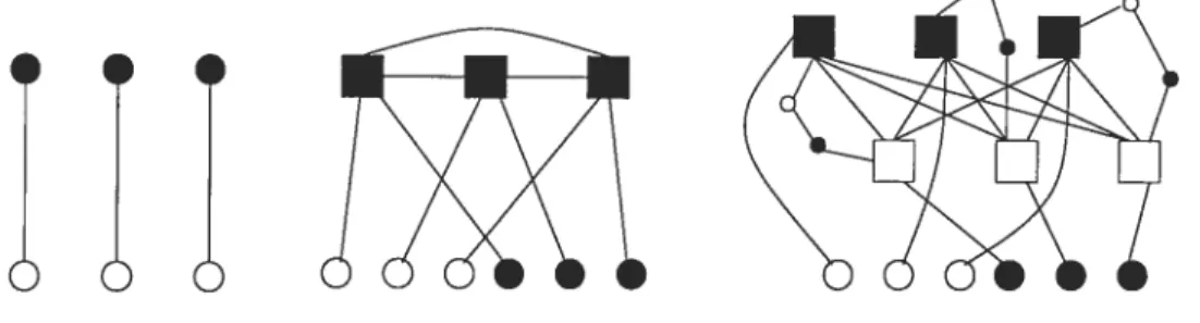
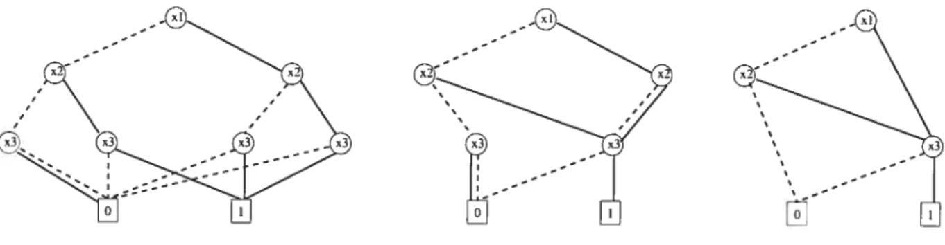
Following this reduction, Nagoya, Uehara auJ Toda [103] construct a cliordal bipartite graph Ç (V.

₎

from the directed path grapli (X U Y U E,

Ê)

in polynomial time. Let V X U Y U E U E’ U B U W. Each vertex e E E corresponds to three vertices

e’ E E’,eb E B, and e E W, respectively. That is, E) = E’) B) W) = ni.

“First, we show how to connect the vertices in E U E’ U B U W.

1. for each vertex e E E, four edges _{{e, e’}, {e’, eb}, {eb, e}. {e, e}} _{are added into S.}

2. for each pair of vertices e1 and e9, {e1, e}. {e. e2} are added into S

Since

Ô[E]

is a clique, Ç[E U _{E’] is a bipartite complete graph. In figure 2.3, black square}

vertices are in E, white square vertices are in E’, srnall black vertices are in B, and small

white vertices are in W.

We recail that the vertices in B U V are not connected to any vertices in X U Y.

“The next step in the construction is to show how to connect the vertices in X and Y to

the vertices in E U E’ UB U 1V as in the example figure 2.3.

(45)

CHAPTER 2. GRAPH ISOMORPHISM ₃₃

2. for each vertex y E Y, {y, e’} is added into if {y, e}

e

Ê.

Then, it is proved that reduced chordal bipartite graph isomorphisrn is polynornially equivalent to directed path graph isomorphism. Given a bipartite graph G, the reduced graph Ç bas n + 4m vertices and rn2 + 5m edges.”

Hence, the chordal bipartite graphs are in isomorphism-complete class.

2.1.4 Self-complementary graph isomorphism

D

Definition 2.3 A (di,)graph G is seÏf-comptementary (sc] if it is isomorphic to its compternent G.

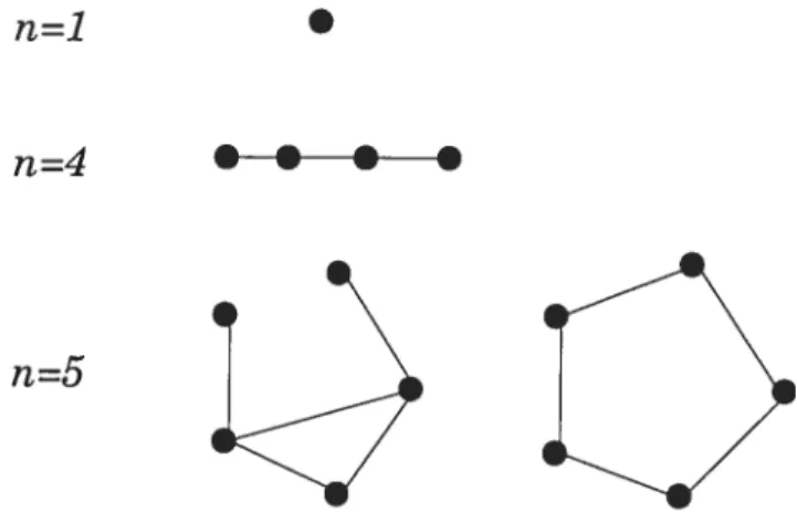
There are relatively few self-cornplementary graphs; on twelve vertices, for instance, only 720 of the 165,091,172,592 graphs are self-complementarv [1131. These are some examples (See Figure 2.1): n=1 n=4 n=5

.

..

.

Theorem 2.4 (Colbourn [37J, 1978)

figure 2.4: self-complementary graphs

(46)

C’HÀP TER 2. GRAPH ISOMORPHISM 34

Proof. For convenience, let s consider Figure 2.5. The problem of determining the isomorphism of two graphs G and H can be polynomially reduced to the recognition of self-compÏementary digraphs. “By reduction, we substitute G for vertex Ï and

R

(graph H’s complement) for vertex 2, and cail the resulting digraph S. Thus, digraph S is self complementar if and only if G and H are isomorphic.”

Figure 2.5: self-complementary digraph

Now, we assume that S is self-complementarv. “In one direction, since everv vertex in

G lias out-degree at least n, whereas any vertex in

R

lias out-degree at most n — 1, any

isomorphism carrying S into must map G into H.”

In the other direction, assume that G is isomorphic to H. “For any isomorphism

_f

mapping G to H. we build the inverse mapping g which is an isomorphism from

R

into . An isornorphism from $ to is constructed bv using the mapping

f

to map vertices from the

portion of S representing G to the portion of representing H, and using mapping g to perfbrm the parallel mapping from

R

to

Ô.

Thus, we can see that S is self-complementary.”

D

Colbourn also show’ed that:

Theorem 2.5 (Colbourn

j37],

1978)

The recognition of setJ-comptementary graphs graph isornorphism.

Theorem 2.6 (Colbourn [37], 1978)

(47)

CHAPTER 2. GRAPH I$OMORPHI$M 35

Similar proofs can be found in

_[31•

2.1.5 Regular graph isomorphism

A graph in which every vertex has the same degree is called regular. If every vertex bas degree k then we say the graph is regular of degree k or k-regular. Nuil graphs are regular of degree zero.

Theorem 2.7 (Booth

[231,

1978)

Regutar graph isomorphism graph somorph2sm.

Proof. Here, we give an outiine of the proof given by Booth

[231.

Since any isomorphism test for arhitrary graplis will also work for regular graphs. we need only show that graph isornorphisrn is polvnornially reclucihie to regular graphs isornorphism. This proofconst.ructs a regiilar graph REG ULAR(G) from any given general graph G and proves that G1 G2

REGULAR(G1) REGULAR(G2).

“Let G (Ç E) be any graph havillg V {u 1 <i <n} and E {e 1

<j

<m} where every vertex belongs to at least one edge and rn — n > 2. Define the following sets:

= {fi 1

j

<m}.

1 km—2},

={kt 1<1< m—n+2}

(48)

CHAPTER 2. GRAPH ISOMORPHISi 36

E1 {{u. e} v _e, 1 <i < n, 1

<j

<m}, E2 = {{v,f}

I

v e,1 <i <n,1

<j

<in}, E3 = {{ej,gk} 1 <k <in—2,1

<j

<m}, E4 {{j,hj 1<1< m—n+2,1

<j

<m}.

Let REGULAR(G) be the graph (VUEUV1ULU, E1UE2UE3uE1). “ We can establish

two facts about REGULAR(G): it isa regular graph of degree in and given REGULAR(G)

we cari recover G uniqueiy.

The first fact is easily verified. “Each v E V lias degree in in REG ULAR(G) because it

is adjacent to either e or

fj

for ail 1 <

j

< in; cadi _e é E lias degree in because it is

adjacent to exactly 2 of the v E V and to ail in— 2 of the 9k ê V2; cadi

f e

V1 is adjacent

to exactiy ‘n — 2 of the v E V and also to ail in — n + 2 of the k, E V3; each 9k E is

adjacent to ail in of the e ê E; finally each li, E is adjacent to ail in of the

J

ê

The second fact follows from the observation that in REGULAR(G) every g, ê V lias exactly tire same set of neighbours and every h, ê lias exactly the same set ofneighbonrs.

“We can teil these two sets apart hecause 1721 > _{1731 since} n > 4 if in — n> 2 in a graph.

Having tins located 17, we know that

E = {vertices at distance 1 from 1},

V = {vertices at distance 2 from 1’}

and also tliat {u,v} E E if and oniy if there is an edge in REGULAR(G) from both

u and V to some e E E. Tic encoding (G1, G2)—÷(REGULAR(G1), REG ULAR(G2)) thus lias the property that G1 G if and oniy if REGULAR(G1)REGULAR(G2). I’vIoreover, it is clearly computable in polynomial time and hence is a polynomial reduction

(49)

CHAPTER 2. GRÀPH ISOMORPHI$M 37

of graph isomorphism to regular graph isomorphism if we realize that isolated vertices can 5e handled with a simple pretest and that adding an eqilal number of copies of 1(4 to both G1 and G2 will not affect their isomorphism but will ensure that in — n > 2, without

increasing the size of the input by more than a polynomial.” E

2.2 Some graph isomorphism problems in

F

As we rnentioned before, although it seerns to be hard to have a polvnomial-time algorithm for general graph isomorphism. many graphs with restrictions are readilv handled. for example. trees, planar graphs, graphs of bounded genus. graphs of hounded valence, graphs of bounded tree-width. graphs of hounded eigenvalue rnultiplicitv and trivalent graphs have polynomial-time algorithms.

The first major resuit in this field was given by Luks j51,

_$81

in 1978. He showeci that graphs with bounded valence can be solved in polynomial time o(nt09k),

where k is the bounded valence. This resuit was obtained by applying powerful group theory. We will give a special presentation of group theory techniques in a later section.

Other interesting graphs are interval graphs.

Definition 2.4 A undirected graph is catÏed interval graph if its vertzces cari be put into one-to-one correspondence with a set of intervaïs of the reat une, such that two vertices are connected by an edge if and onïy if their corresponding intervats have nonempty intersection.

Interval graphs can be tested for graph isomorphism in O(mn), where m is the number of edges and n is the number of vertices, following resuits h Hsu j69] in 1995. Compared to other resuits, this result is very interesting in that it does flot require some explicit

(50)

CHAPTER 2. GRAPH ISOMORPHISAi _3$

C

parameter to be fixed (constallt) which is often required by many polynomial algorithms, and seems feasible to apply to a large and practical group of graphs [51J.

In the following sections, several major resuits in the graph isornorphisrn problem will he shown using two approaches: combinatorial approach and group-theoretic approach. Ail of these resuits are in polyllomial time at most; some of them are even in linear time or atternating Ïogtime (Atogtirne). We discuss this problem in the next section.

2.3 Combinatorial approach

2.3.1 Tree

isomorphism

As we have seen, a tree is a finite, conllected, acyclic graph. Tree isomorphism is the basis of naïve solutions to the more general problems of subtree isomorphism, largest common subtree, and perhaps aiso smallest common super-tree.

Trees isomorphism bas been studied since the 1970’s. first, in 1974, Aho, Hopcroft and Uliman [2] gave a linear-time aigorithm for tree isomorphism, based on comparing two trees in a bottom-up fashion. Certainly, linear time is the best possible sequential run time for tree isomorphism, but it is possible to consider refined algorithms, sav parallel run. in smaller complexity classes

[321,

for instance, the class NC. In 1981, Ruzzo [1161 found an NC-algorithm for solving the tree isomorphism problem for trees of logarithmic degree. Later, in 1991, Miller and Reif [100] mentioned an NC-aigorithm for this problemproblem and the tree canonization problein for trees of arbitrary degree and depth. Further, Lindell

[$61

showed deterministic logarithmic-space algorithms for the tree isomorphism, tree comparison and tree canonization problems. Finaiiy, in 1997, Buss [32] gave an aÏternating

(51)

CHAPTER 2. GRÀPH ISOAiORPHISM 39

togtime (Àlogtime) algorithm for tree isomorphisrn. In this surve, we shah show the idea of Buss Alogtime algorithm.

Prelimirraries and definitions

Definition 2.5 [2J The cÏass of tanguages accepted by ATMs within tiine O(logn) is catted Alogtime.

Definition 2.6 An immediate snbtree of T is a subtree whose root is a chitd ofT’s root vertex.

Definition 2.7 [32J Let $ and T be trees. We define $ T, caÏted tree equatity, by induction on the number of vertices in S and T by defining that S T hotUs if ccnd onÏy if

1. S T = 1 or

2. S and T both have the same number, in, of immediate subtrees, and theTe is some ordering 5i , 5m of the immediate subtrees of S and sorne ordering T1, Tm of

the immediate subtrees of T such that $ T,Vi, 1 < j < m.

It is easv to check that $ T if and only if there is an isornorphisrn of $ and T.

Definition 2.8 Let S and T be trees. We define S - T and S - T, catted tinear ordering of trees, sirnuttaneousÏy by induction on the size of $ and T. The tinear ordering $ -< T hotUs if and onÏy either $ - T or $ T. The tinear ordering $ -< T hoÏds if and onÏy if either $ < T hotds or the foïtowing conditions hotU:

(52)

CHAPTER 2. GRAPH ISOMORPHISM 40

1. S = T, and

2. Let $, Si,, be the irnrnediate snbtrees of S ordered so that 5m 5m—i S, and let T1, ,T be the immediate s’izbtrees of T. szrnzlarty oTdered with T1 — T

for alt j. Then

(a) For sorne j <inin{rn,n},S - I and for ahi

<j

T, or (b) rn<n andISforattl <i<rn.

Miller and Reif 1100] introduced a method to represent trees by strings over the two symbol alphabet containing open and close parentheses. The tree with a single vertex is denoted by the string

_“Q”.

If T is a tree with more than oiie vertex, ifcr1, _orn are strings representing the immediate subtrees, then “(ou,. , n)” is a string representation of tree T.

Hence, the isomorphism of trees becornes the problem of determining whether two input strmg representations are isomorphic.

The basic idea of the algorithm

It is knowri that Alogtime algorithms are capable of parsing parenthesis languages. for more information on these aspects of Àlogtime, readers are advised to consuit

_[311.

Particularly, by counting parentheses, an Alogtime algorithm can compute the depth of a vertex in a tree, can determine the i-th child of any vertex in a tree and know the ancestor/descendant predicates, etc. Also, Alogtime algorithms are capable of converting hetween prefix and infix notations [32].

Definition 2.9 Let S be a subtree of a tree T. Let T = T0. T1. , T = S be the (unique)

(53)

CHAPTER 2. GRAPH ISOMORPHISM 41

signature of_{S in T is defined as the sequence (ToL T1,} , Tk). IfS’ is a subtree of a tree T’, then S and S’ are simitar provided:

1. They have the same size-signature, and 2. They are isomorphic, i.e., $ S’.

It is easy to see that the size-signature is invariant under isomorphism. By parsing and counting techniques, tl1ere is an Alogtime procedllre which, from a string representation of a tree T and a given subtree $ of T, can generate the size-signature of S in _{T 132].}

Let logn denote the logarithrn (in base 2) of n rounded down to the integer. The logsize. togsize(T), of a tree T is deflned to equal log jT.

Definition 2.10 Let T1,T2 be non-equat and non zso’rnorphic trees. LetS be a subtree of

Ty. We say that S dist’inguishes T1 fro’m T2 pro vided that S is a proper subtree ofî and:

1. The togsize of S is strictty Ïess than the Ïogsize of the parent tree of S, and

2. The number of snbtrees of T1 which are sirnitar to S is not equat to the nwrnber of

subtrees of T2 which are simitar to S.

Now, we present the idea of tree isomorphism algorithm in the help of the representation of trees.

“We can view an Alogtime algorithm as a garne between two players: the first player is asserting that the two trees are non-isomorphic, while the second player is asserting that the two trees are isornorphic. The input to the game consists oftwo string representations

A survey of graph and subgraph isomorphism problems

Université de Montréal

A survey

of

Vo5

graph and subgraph isomorphism problems

par

Yaohui Lei

)ûQL

Université

dl1

de Montréal

Université de Montréal

Faculté des études supérieures

A survey

graph and subgrapb isomorphism problems

Yaohui Lei

À

Contents

C

List of Figures

List of Algorithms

Chapter 1

Introduction and Preliminaries

1.1

Introduction

1.1.1

Graph isomorphism

[•51

1791

1791

891.

1.1.2

Subgraph isomorphism

1.2

Basic computational complexity

f,

e

e

1.2.1

Turing machine

4.

Q

e

Q

Q

e Q

Q

(Q,

Q

Q

Q

Q

Q

e Q

(Q,

(Q

Q

e

Q

)

1.2.2

Decision problems

+

f

1.2.3

Polynomial reductions and transformations

1.2.4

The classes P, NP, NP-hard and NP-complete

1.2.5

The class NC

1.3

Group theory preliminaries

.),

e

e

e

e

f

)

_[•51

₁₇₉₁

_f,

_Q

_e

_Q

_Q

_Q

_Q

_Q

_(Q,

_Q

₎

_f

_[251

_),

_f

_f

_1141,

_1781.

_[231,

_[31

_115].

_(,

_G

₎