High resolution RCS imaging in anechoic chamber by introducing a random medium

HAL Id: tel-01765346

https://tel.archives-ouvertes.fr/tel-01765346

Submitted on 12 Apr 2018

HAL is a multi-disciplinary open access archive for the deposit and dissemination of sci-entific research documents, whether they are pub-lished or not. The documents may come from teaching and research institutions in France or abroad, or from public or private research centers.

L’archive ouverte pluridisciplinaire HAL, est destinée au dépôt et à la diffusion de documents scientifiques de niveau recherche, publiés ou non, émanant des établissements d’enseignement et de recherche français ou étrangers, des laboratoires publics ou privés.

Stefania Bucuci

To cite this version:

Stefania Bucuci. High resolution RCS imaging in anechoic chamber by introducing a random medium. Signal and Image processing. Université Rennes 1; Universite de rennes 1, 2017. English. �NNT : 2017REN1S108�. �tel-01765346�

THÈSE / UNIVERSITÉ DE RENNES 1

sous le sceau de l’Université Bretagne Loire pour le grade de

DOCTEUR DE L’UNIVERSITÉ DE RENNES 1

Mention : Traitement de Signal et Télécommunications

Ecole doctorale MathSTIC

Ștefania Bucuci

Préparée à l’unité de recherche IETR (UMR CNRS 6164)

Institut d’Electronique et de Télécommunications de Rennes

Université de Rennes 1

Imagerie Haute

Résolution SER en

Chambre Anéchoïque

grâce à l’introduction

d’un Milieu Diffusant

Thèse soutenue vue à Rennes le 21/12/2017

devant le jury composé de : Elodie RICHALOT

Professeure à l’Université Paris-Est Marne-la-Vallée

/ rapporteur

Cyril DECROZE

Maître de Conférences à l’Institute de recherche XLIM / rapporteur

Joseph SAILLARD

Professeur à l’Université de Nantes / examinateur Philippe POULIGUEN

Responsable du Domaine Scientifique de la MRIS « Ondes Acoustiques et Radioélectriques » /

examinateur

Patrick POTIER

Docteur DGA/MI à Bruz / examinateur Ala SHARAIHA

Professeur à l’Université de Rennes 1 / directeur de thèse

Matthieu DAVY

Maître de Conférences à l’Université de Rennes 1 / co-directeur de thèse

i

Quote

“Science is made up of mistakes, but they are mistakes which it is

useful to make, because they lead little by little to the truth.”

iii

Acknowledgements

This manuscript presents the work carried out at Institute of Electronics and Telecommunications of Rennes with the financial support of the Direction Générale de l‟Armement (DGA).

Foremost, I would like to express my sincere gratitude to Prof. Elodie Richalot and Dr. Cyril Decroze for doing me the honor to be the reviewers of my PhD thesis. I am grateful for their detailed review of the manuscript that helped me improve and complete my thesis. As well, I would like to thank Prof. Joseph Saillard who has agreed to be the president of my thesis jury and I am deeply appreciative to all jury members, namely Dr. Philippe Pouliguen and Dr. Patrick Potier for consenting to read the manuscript.

Moreover, I would like to present my profound gratitude to my supervisor Prof. Ala Sharaiha for his continuous support of my PhD study and research, for his motivation and his vast knowledge.

Besides, I would like to convey my great appreciation for my co-supervisor Dr. Matthieu Davy for his patience and guidance which helped me in all the time of research.

Besides my advisors, I would like to express my gratitude to Dr. Philippe Pouliguen for his encouragement and insightful comments during my study.

I am also grateful for all the support I received from all the members from the lab: the IETR director, the secretaries and mechanics. Their help has facilitated my work throughout my thesis.

I was fortunate to have kind colleagues especially Mr. Jerome Sol from National institute of Applied Sciences of Rennes (INSA) and Mr. Frédéric Boutet from IETR, who helped me and provided me all the apparatus I needed for measurements.

I also want to thank my fellow lab mates for the pleasant time we had in the last three years and for their support. Special thanks go to Laura Pometcu, a wonderful colleague who always helped me and to Dr. Mohsen Koohestani, an awesome colleague who had been always there to support and encourage me.

Last but not least, I would like to thank my family and friends for all their encouragement, support and motivation. Here, another special thanks goes to Prof. Răzvan Tamaş from Constanţa Maritime University.

v

Contents

List of Figures xiii

Résumé

Introduction

CHAPTER 1

Radar cross section principles

1.2 Radar basic definitions ... 5

1.2.1 History of radar ... 5

1.2.2 Introduction to radar systems... 6

1.2.3 Radar equation ... 9

1.3 Radar cross section fundamentals ... 10

1.3.1 Radar cross section determination ... 10

1.4 Scattering regimes ... 13

1.4.1 Low-frequency scattering region ... 13

1.4.2 Mie resonant scattering region... 14

1.4.3 High-frequency optical scattering region ... 15

1.5 Calibration targets ... 16

1.5.1 Flat plate ... 16

1.5.1.1 Rectangular flat plate ... 16

1.5.1.2 Circular flat plate ... 17

1.5.2 Dihedral reflector ... 18

1.5.3 Trihedral reflector ... 20

1.5.3.1 Rectangular trihedral reflector ... 20

1.5.3.2 Circular trihedral reflector ... 21

vi

1.6 Polarization scattering matrix ... 23

1.7 Radar cross section measurements ... 25

1.7.1 Measurement facilities ... 26

1.7.1.1 Indoor facilities and anechoic chamber – far field range ... 26

1.7.2 Radar cross section imagery ... 29

1.7.2.1 One-dimensional range profile ... 29

1.7.2.2 One-dimensional cross-range profile ... 31

1.7.2.3 Two-Dimensional ISAR image ... 33

1.8 Conclusion ... 36

CHAPTER 2

Time reversal technique

2.2 Time reversal in acoustics ... 40

2.2.1 Wave equation ... 40

2.2.2 Time reversal cavity ... 41

2.2.3 Time reversal mirror ... 45

2.2.4 Time reversal in random media ... 46

2.2.5 Time Reversal in a waveguide ... 49

2.2.6 Time Reversal in a chaotic cavity ... 51

2.3 Time reversal in electromagnetics ... 52

2.3.1 Time-symmetry of electromagnetic waves ... 53

2.3.2 Reciprocity of electromagnetic waves ... 54

2.3.3 Electromagnetic time reversal cavity... 55

2.3.4 Time Reversal within a reverberation chamber ... 57

2.3.5 Radar imaging using a time reversal beamformer ... 60

2.4 Time reversal focusing through a random medium ... 63

2.4.1 Basics of the finite-difference time-domain method ... 64

2.4.1.1 FDTD grid ... 64

2.4.1.2 Boundary conditions ... 65

2.4.2 The finite-difference time-domain simulations ... 65

2.4.2.1 Focusing on a position ... 65

2.4.2.2 Focusing on multiple positions ... 73

vii

CHAPTER 3

Modeling of a microwave imaging system using a random

medium

3.1 Introduction ... 77

3.2 Microwave imaging ... 77

3.3 Conception and design of the medium ... 79

3.3.1 First trial - rod diameter: 10 mm ... 79

3.3.2 Second trial - rod diameter: 15 mm ... 81

3.3.3 Third trial - rod diameter: 20 mm ... 83

3.4 Target detection through a random medium 2D simulations ... 85

3.4.1 Random medium characteristics ... 85

3.4.2 First simulation setup: Setup A ... 90

3.4.2.1 Time reversal method ... 92

3.4.2.2 Matrix inversion method ... 93

3.4.3 Second simulation setup: Setup B ... 97

3.4.3.1 Time reversal method ... 98

3.4.3.2 Matrix inversion method ... 99

3.4.4 Comparison of different metallic boundaries on simulation setup A ... 100

3.4.4.1 Time reversal method ... 103

3.4.4.2 Matrix inversion method ... 105

3.5 Conclusion ... 109

CHAPTER 4

Imaging through a random medium using two antennas

4.2 Random medium fabrication ... 111

4.3 Experimental results ... 113

4.3.1 Measurement setup ... 113

4.3.2 Multiple antennas measurement setup ... 121

4.3.2.1 Case 1 – one antenna emitting through the medium ... 124

4.3.2.2 Case 2 – two antennas emitting through the medium ... 129

4.3.2.3 Case 3 – three antennas emitting through the medium ... 133

4.4 Conclusion ... 136

General conclusion and future work

Communication and publication

ix

Acronyms

1D One-Dimensional

2D Two-Dimensional

3D Three Dimensional

ABC Absorbing Boundary Conditions

CW Continuous Waveform

FFT Fast Fourier Transform

FM Frequency modulation

FDTD Finite-Difference Time-Domain

HF High Frequency

HH Horizontal-Horizontal

HV Horizontal-Vertical

IETR Institute of Electronics and Telecommunications of Rennes

IFT Inverse Fourier Transform

ISAR Inverse Synthetic Aperture Radar

LL Left-Left

LR Left-Right

MI Matrix Inversion

NTF Near-to-Far-field Transformation PEC Perfect Electrical Conductor

PML Perfectly Matched Layers

RADAR RAdio Detection and Ranging

RCS Radar Cross Section

RF Radio Frequency

x RR Right-Right SNR Signal-to-Noise Ratio TE Transverse Electric TM Transverse Magnetic TR Time Reversal

TRM Time Reversal Mirror

UHF Ultra High Frequency

U.K. United Kingdom

U.S. United States

UWB Ultra Wide Band

VH Vertical-Horizontal

VHF Very High Frequency

xi

List of Tables

Table 1.1 Radar frequency bands [6] ... 9

Table 1.2 Polarization cases... 25

Table 2.1 Random medium - focal spot dimensions for different apertures of TRM ... 71

Table 2.2 Free space - focal spot dimensions for different apertures of TRM ... 72

Table 3.1 First trial - The number of rods and the distances between them ... 79

Table 3.2 Second trial - The number of rods and the distances between them ... 81

xiii

List of Figures

Figure 1 La configuration de simulation: a) le premières deux étapes; b) la troisième

étape ... xxi

Figure 2 La reconstruction de la surface scannée – Retournement temporel ... xxi

Figure 3 Les lobes secondaires – Retournement temporel ... xxii

Figure 4 La reconstruction de la surface scannée – Inversion matricielle ... xxiii

Figure 5 Les lobes secondaires – Inversion matricielle ... xxiii

Figure 6 La configuration de mesure : a) la première étape ; b) la deuxième étape ... xxv

Figure 7 Detection de la position du triedre : a) ; b) ; c) ; d) ; e) ; ... xxvii

Figure 1.1 Radar working principle ... 7

Figure 1.2 Monostatic radar: ... 11

Figure 1.3 Bistatic radar ... 12

Figure 1.4 Forward scatter radar ... 12

Figure 1.5 Normalized RSC of a metallic sphere over the three scattering regimes ... 13

Figure 1.6 Square plate ... 17

Figure 1.7 Simulated monostatic RCS of a flat square plate ... 17

Figure 1.8 Circular plate ... 18

Figure 1.9 Simulated monostatic RCS of a flat circular plate ... 18

Figure 1.10 Dihedral reflector ... 19

Figure 1.11 Simulated monostatic RCS of a dihedral reflector ... 19

Figure 1.12 Rectangular trihedral reflector ... 20

Figure 1.13 Simulated monostatic RCS of a rectangular trihedral reflector ... 20

Figure 1.14 Circular trihedral reflector ... 21

Figure 1.15 Simulated monostatic RCS of a circular trihedral reflector ... 21

Figure 1.16 Triangular trihedral reflector ... 22

Figure 1.17 Simulated monostatic RCS of a triangular trihedral reflector ... 23

Figure 1.18 SOLANGE indoor RCS range [19] ... 26

Figure 1.19 CHEOPS anechoic chamber ... 26

Figure 1.20 Anechoic room schematic – top view ... 27

Figure 1.21 Tapered anechoic room schematic – top view ... 28

xiv

Figure 1.23 Range profile of a model airplane [24] ... 31

Figure 1.24 Cross-range profile [24] ... 32

Figure 1.25 Cross range profile of a model airplane [24] ... 33

Figure 1.26 Geometry for monostatic ISAR imaging [24] ... 34

Figure 2.1 Time reversal process using time reversal cavity: - first step ... 43

Figure 2.2 Time reversal process using time reversal cavity: - second step ... 44

Figure 2.3 Time reversal process using time reversal mirror: - first step ... 45

Figure 2.4 Time reversal process using time reversal mirror: - second step ... 45

Figure 2.5 Time reversal process using a random medium: - first step ... 46

Figure 2.6 Time reversal process using a random medium: - second step ... 47

Figure 2.7 The aperture of TRM in homogeneous medium ... 47

Figure 2.8 The virtual aperture of TRM using a random medium ... 48

Figure 2.9 Example of time signal registered on TRM ... 48

Figure 2.10 Waveguide experiment schematic ... 49

Figure 2.11 Waveguide - temporal signals [45]: ... 50

Figure 2.12 Directivity pattern [45] ... 50

Figure 2.13 The principle of mirrors ... 50

Figure 2.14 Chaotic cavity experimental setup ... 51

Figure 2.15 Chaotic cavity - time signals [41]: ... 52

Figure 2.16 Time reversal process using electromagnetic time reversal cavity: first step . 56 Figure 2.17 Time reversal process using electromagnetic time reversal cavity: second step ... 57

Figure 2.18 Reverberation chamber at IETR research laboratory ... 58

Figure 2.19 Time signals corresponding to measurement steps [55] ... 59

Figure 2.20 Total efficiency [55] ... 60

Figure 2.21 Principle of a passive beamformer [61] ... 61

Figure 2.22 Experimental beamformer [61] ... 62

Figure 2.23 Radiation pattern [61] ... 63

Figure 2.24 a) Radar imaging setup; b) radar imaging using TR beamformer [61] ... 63

Figure 2.25 FDTD simulation setup: a) first step; b) second step ... 66

Figure 2.26 Emitted pulse ... 66

Figure 2.27 First step of time reversal FDTD simulation: a) emitting source; ... 67

Figure 2.28 Time signal recorded on TRM ... 67

xv

Figure 2.30 Time signal recorded on source location ... 69

Figure 2.31 3D focal spot ... 70

Figure 2.32 2D focal spot ... 70

Figure 2.33 Focal spot dimensions – 61 elements TRM: ... 70

Figure 2.34 Focal spot dimensions – 1 element TRM in free space ... 72

Figure 2.35 Focal spot dimensions – elements TRM ... 72

Figure 2.36 FDTD simulation setup: a) first step; b) second step ... 73

Figure 2.37 Multiple foci ... 73

Figure 2.38 Merged foci: a) one wide focus; b) three wide foci; c) three merged foci in different planes ... 74

Figure 3.1 Microwave imaging hardware system schematic ... 78

Figure 3.2 Test configuration ... 80

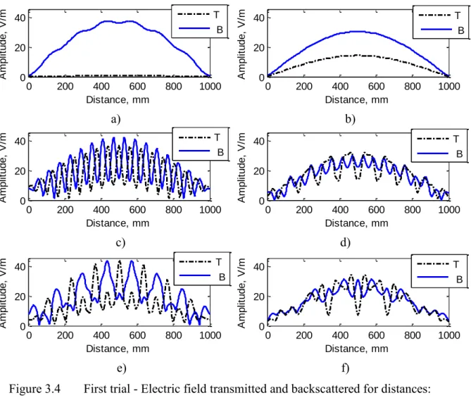
Figure 3.3 First trial - Electric field surface for distances: a) ; b) ; c) ; d) ; e) ; f) ; ... 80

Figure 3.4 First trial - Electric field transmitted and backscattered for distances: a) ; b) ; c) ; d) ; e) ; f) ; ... 81

Figure 3.5 Second trial - Electric field surface for distances: a) ; b) ; c) ; d) ; e) ; f) ; ... 82

Figure 3.6 Second trial - Electric field transmitted and backscattered for distances: a) ; b) ; c) ; d) ; e) ; f) ; ... 83

Figure 3.7 Third trial - Electric field surface for distances: a) ; b) ; c) ; d) ; e) ; f) ; ... 84

Figure 3.8 Third trial - Electric field transmitted and backscattered for distances: a) ; b) ; c) ; d) ; e) ; f) ; ... 85

Figure 3.9 2D Time reversal configuration ... 86

Figure 3.10 Surface electric field plot ... 86

Figure 3.11 Electric field amplitude versus frequency ... 87

Figure 3.12 Time signal on TRM ... 87

Figure 3.13 Spatial correlation function ... 88

Figure 3.14 Spectral correlation function ... 90

Figure 3.15 First 2D simulation setup: ... 91

Figure 3.16 Reconstruction of scanned area using TR method – Setup A ... 92

xvi

Figure 3.18 Distribution of singular values of matrix ... 94

Figure 3.19 SNR ... 95

Figure 3.20 Reconstruction of scanned area using MI method – Setup A ... 96

Figure 3.21 Sidelobes amplitude using MI method – Setup A ... 96

Figure 3.22 Second 2D simulation setup: ... 97

Figure 3.23 Reconstruction of scanned area using TR method – Setup B ... 98

Figure 3.24 Sidelobes amplitude using TR method – Setup B ... 99

Figure 3.25 Reconstruction of scanned area using MI method – Setup B ... 99

Figure 3.26 Sidelobes amplitude using MI method – Setup B ... 99

Figure 3.27 Scanning configuration: a) version 1; b) version 2; c) version 3 ... 100

Figure 3.28 DUT configuration: a) version 1; b) version 2; c) version 3 ... 100

Figure 3.29 Electric field amplitude versus frequency: a) version 1; b) version 2; c) version 3 ... 101

Figure 3.30 Spectral correlation function: a) version 1; b) version 2; c) version 3 ... 102

Figure 3.31 Reconstruction of scanned area using TR method: ... 104

Figure 3.32 Sidelobes amplitude using TR method: ... 105

Figure 3.33 Distribution of singular values of matrix ... 106

Figure 3.34 Reconstruction of scanned area using MI method: ... 107

Figure 3.35 Sidelobes amplitude using MI method: ... 108

Figure 4.1 Fabricated medium parts schematic ... 111

Figure 4.2 Fabricated random medium schematic ... 112

Figure 4.3 Fabricated random medium: a) top view; b) side view ... 113

Figure 4.4 Measurement setup: ... 114

Figure 4.5 parameters at central frequency: a) ; b) ... 115

Figure 4.6 Schematic setup: ... 116

Figure 4.7 Reconstructed area: ... 117

Figure 4.8 Reconstruction of area F using MI method – Measurement setup: ... 119

Figure 4.9 Sidelobes amplitude MI vs TR method: ... 121

Figure 4.10 Multiple antennas measurement setup: ... 122

Figure 4.11 Multiple antennas schematic setup: ... 123

Figure 4.12 Reconstructed area: ... 124

Figure 4.13 Multiple antennas schematic - case 1: ... 125

Figure 4.14 Reconstruction of area F using TR method – Multiple antennas measurement setup: a) case 1.1; b) case 1.2; c) case 1.3 ... 126

xvii

Figure 4.15 Reconstruction of area F using MI method – Multiple antennas measurement setup: a) case 1.1; b) case 1.2; c) case 1.3 ... 127 Figure 4.16 Sidelobes amplitude MI vs TR method – Multiple antennas measurement

setup: a) case 1.1; b) case 1.2; c) case 1.3 ... 128 Figure 4.17 Multiple antennas schematic - case 2: ... 129 Figure 4.18 Reconstruction of area F using TR method – Multiple antennas measurement

setup: a) case 2.1; b) case 2.2; c) case 2.3 ... 130 Figure 4.19 Reconstruction of area F using MI method – Multiple antennas measurement

setup: a) case 2.1; b) case 2.2; c) case 2.3 ... 131 Figure 4.20 Sidelobes amplitude MI vs. TR method – Multiple antennas measurement

setup: a) case 2.1; b) case 2.2; c) case 2.3 ... 132 Figure 4.21 Multiple antennas schematic: Case 3 ... 133 Figure 4.22 Reconstruction of area F using TR method – Multiple antennas measurement

setup: Case 3 ... 133 Figure 4.23 Reconstruction of area F using MI method – Multiple antennas measurement

setup: Case 3 ... 134 Figure 4.24 Sidelobes amplitude MI vs. TR method – Multiple antennas measurement

setup: Case 3 ... 134 Figure 4.25 Comparison for the three cases - TR method: a) amplitude; b) sidelobes ... 135 Figure 4.26 Comparison for the three cases - MI method: a) amplitude; b) sidelobes ... 135 Figure 4.27 Comparison between coherent and incoherent sum of images - TR method:

xix

Résumé

Les mesures utilisées actuellement en chambres anéchoïque, pour la caractérisation de la surface équivalente radar (SER) des antennes ou des objets sont généralement perturbées, en particulier en basse fréquence lorsque les longueurs d‟onde sont supérieures au mètre. L‟épaisseur des matériaux absorbants devient faible devant la longueur d‟onde et ceux-ci ne peuvent plus être considérés comme parfaitement absorbants. Les parois de la chambre (murs, plafond, sol) qui sont illuminées génèrent des trajets multiples. Dans ce cas, le champ total incident sur la cible sous test est la somme du champ incident direct et des champs réfléchis par les parois.

Ce résume de la thèse présente une nouvelle technique d‟illumination permettant de focaliser le champ incident sur la zone utile occupée par la cible. Nous présentons la méthodologie utilisée et la configuration proposée en simulations. L‟analyse des résultats expérimentaux est aussi réalisée.

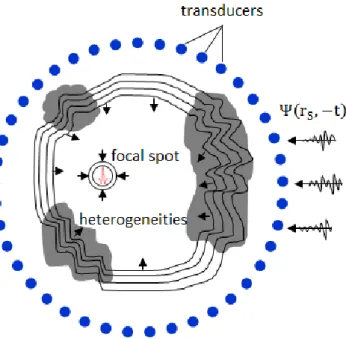
La méthode se base sur le principe de retournement temporel (RT) qui permet de focaliser spatialement et temporellement une onde électromagnétique. Dans une première phase d‟enregistrement, une source émet un signal très bref qui est diffusé à travers un milieu dispersif. Le signal est enregistré sur un réseau d‟antennes, le miroir à retournement temporel (MRT). Puis, les signaux inversés temporellement sont réémis afin de focaliser l‟onde à la position de la source initiale.

Un signal à large bande transmis à travers un milieu complexe s‟étale sur un temps beaucoup plus long que la durée du signal incident du fait de la propagation multi-trajets dans le milieu. Du fait de la diffusion multiple des ondes, le signal aux temps longs semble complètement aléatoire. Néanmoins, l‟onde ne perd pas sa cohérence. L‟information spatiale donnée par les temps longs fournit une grande diversité spatiale qui est exploitée pour focaliser les ondes avec une résolution fine dans la deuxième phase du retournement temporel. L‟intensité focalisée est la somme de l‟intensité directe et l‟intensité diffuse qui décroit en fonction de la distance parcourue à travers le milieu diffusant.

La performance de focalisation du RT à travers un milieu complexe peut être caractérisée par le rapport entre l'amplitude du signal focalisé et l'amplitude des lobes secondaires. Ce rapport est égal au nombre de degrés de liberté spatio-temporels.

Considérons la transmission à travers un milieu aléatoire de longueur qui peut être caractérisé par le libre parcours moyen . Le libre parcours moyen est lié au coefficient de

xx

diffusion du milieu par , où est la vitesse de transport des ondes et la dimension du milieu. La transformée de Fourier de la réponse impulsionnelle de la source à un élément du MRT peut s‟écrire comme :

( ) 〈 ( )〉 ( ) ₍₁₎

où 〈 ( )〉 correspond à la réponse impulsionnelle cohérente et ( ) donne l‟apport de la partie incohérente. Les contributions de ces termes sont alors donnés par:

|〈 ( )〉| ₍₂₎

〈| ( )| 〉 ₍₃₎

Si , le signal est dominé par la contribution incohérente et la taille de la tache focale ne dépend plus de l‟ouverture du réseau d‟antennes émettrices mais de l‟ouverture du milieu diffusant. Pour des signaux large-bande, il est ainsi possible de focaliser les ondes en utilisant un unique élément du MRT.

Le milieu complexe à deux dimensions proposé en simulations est une forêt de tiges métalliques de diamètre . La bande de fréquence considérée est comprise entre 5 et 7 GHz. La largeur du milieu est de et la longueur est de pour la fréquence centrale de . La distance minimale entre les tiges est de .

La configuration du milieu est présentée sur la Figure 1. Deux port en émission/réception ( et ) sont considérées. La simulation se déroule en trois étapes. Dans les deux premières étapes les champs électriques correspondant à une émission par puis , notés ( ) et ( ) sont enregistrés sur une surface de par devant le milieu. De plus, la transmission entre les deux ports, ( ) sans cible est enregistrée.

Dans la troisième étape de simulation, une sphère métallique, est ajoutée à l‟intérieur de la surface scannée précédemment et nous enregistrons la transmission entre les deux ports,

( ) avec la cible. La différence entre les deux paramètres enregistrés ( ) et ( )

donne le paramètre contenant la rétrodiffusion de la cible, en présence du milieu.

En supposant que le coefficient de diffusion de la cible est indépendant de la fréquence ( ) ( ), le paramètre ( ) - ( ) peut être écrit sous l‟approximation de

Born comme :

( ) ∫ ( ) ( ) ( ) (4)

xxi

a) b)

Figure 1 La configuration de simulation: a) le premières deux étapes; b) la troisième étape

Nous utilisons d'abord une méthode de RT pour imager la cible. Le signal focalisé est obtenu par convolution dans le domaine temporel, qui devient dans le domaine fréquentiel une multiplication de ( ) par le produit des deux champs électriques enregistrés sur la

surface scannées pour chaque port. Pour chaque position scannée dans les deux premières étapes, on exprime l‟image par:

( ) | ( ) ( ) ( ) | (5)

Les équations (4) et (5) montrent que pour une cible ponctuelle située à la position , les interférences constructives des fréquences dans la bande passante donnent une forte intensité à cette position. Au contraire, pour les positions , les interférences doivent être destructives. La reconstruction de la surface scannée pour la troisième étape de simulation est présentée sur la Figure 2.

Figure 2 La reconstruction de la surface scannée – Retournement temporel

Distance, mm D is ta n c e , m m 0 200 400 600 800 1000 600 700 800 900 0.2 0.4 0.6 0.8 1

xxii

La cible, une sphère métallique ajoutée à l‟intérieur de la surface scannée est détectée et localisée à la position ( ). Des lobes latéraux sont observés dans cette configuration lors de la focalisation du signal sur la position de la cible. La Figure 3 montre l‟amplitude des lobes secondaires.

Figure 3 Les lobes secondaires – Retournement temporel

La présence de la cible est détectée à la position . Les lobs secondaires peuvent être observés sur les positions adjacentes sur l‟abscisse.

Puisque les lobes latéraux sont inhérents à la méthode de retournement temporel, nous utilisons une méthode basée sur une inversion matricielle qui fournit des lobes secondaires plus faible.

En supposant que le coefficient de rétrodiffusion de la cible dépend à peine de la fréquence sur la gamme de fréquences utilisés et afin d‟améliorer la détection, nous écrivons l‟équation (4) sous une forme matricielle :

(6)

La matrice est le produit des deux champs électriques enregistrés :

( ) ( ). Dans cette équation, pour trouver l‟inconnue, , il est nécessaire d‟inverser la matrice :

(7)

L‟inversion de la matrice necesite une décomposition en valeur singulières (SVD), . et sont les matrices des valeurs singulières orthonormées. est une matrice diagonale contenant les valeurs singulières de la matrice . L‟expression de la matrice inverse est donnée par :

0 200 400 600 800 1000 0.2 0.4 0.6 0.8 1 Distance, mm A m p lit u d e , V /m

xxiii

(8) Néanmoins dans ce cas, un poids significatif est donné aux valeurs singulières faibles et la procédure d‟inversion peut devenir instable en présence de bruit.

Une méthode de régularisation doit ainsi être appliquée. Nous appliquons la méthode de la SVD tronquée en rejetant les plus petites valeurs singulières. Une autre méthode de régularisation est la régularisation de Tikhonov. Dans ce cas, l‟image est estimée par :

̃ ( )

(9)

où , est le paramètre de régularisation et est la matrice identité.

La Figure 4 présente la reconstruction de la surface scannée pour la troisième étape de simulation.

Figure 4 La reconstruction de la surface scannée – Inversion matricielle

La cible est détectée et localisée et les lobes secondaires ont été fortement atténués par rapport à la méthode du retournement temporel. La Figure 5 montre l‟amplitude des lobes secondaires.

Figure 5 Les lobes secondaires – Inversion matricielle

Distance, mm D is ta n c e , m m 0 200 400 600 800 1000 600 700 800 900 0 0.5 1 0 200 400 600 800 1000 0 0.2 0.4 0.6 0.8 1 Distance, mm A m p lit u d e , V /m

xxiv

La présence de la cible est détectée à la position . Une nette amélioration des lobes secondaires peut être observée.

La configuration de mesure est similaire à la configuration de simulation. Le milieu est encadré par deux antennes cornet et derrière et devant le milieu. Une troisième antenne omnidirectionnelle et large bande est utilisée pour scanner le champ sur une ligne. La longueur de la ligne scannée est d‟un mètre et les paramètres sont enregistrés sur positions de à .

Les caractéristiques physiques de milieu sont les mêmes. Les tiges d‟acier ont un diamètre . La largeur du milieu est de et la longueur est de pour la fréquence centrale de . La distance minimale entre les tiges est de . La hauteur des tiges est bien supérieure à afin de se positionner dans une configuration quasi-2D.

Les mesures seront effectuées en deux étapes. Dans la première étape, l‟antenne scanne le champ devant le milieu diffusant sur une ligne, tandis que les antennes et sont en émission. Pour chaque position de , tous les paramètres sont enregistrés. La transmission entre les deux antennes et , le paramètre ( ) sans cible est aussi

enregistrée. Dans la deuxième étape de la configuration de mesures, la troisième antenne est remplacée par la cible, dans ce cas, un trièdre. La cible est déplacée sur 10 positions de à afin de vérifier la concordance des positions estimées et des positions réelles. La transmission entre les deux antennes et , le paramètre ( ) avec la cible est

enregistrée. La différence entre les deux paramètres enregistrés donne le paramètre contenant la rétrodiffusion de la cible.

La configuration pour les deux étapes de mesures est présentée sur la Figure 6.

xxv b)

Figure 6 La configuration de mesure : a) la première étape ; b) la deuxième étape A partir du scan du champ le long d‟une ligne, nous pouvons reconstruire le champ émis par les antennes devant et derrière cette ligne afin d‟obtenir le champ en toute position de l‟espace. La re-propagation du champ scanne sur la ligne est réalisée grâce à la somme cohérente des signaux multiplies par les fonctions de Green 3D :

( )

( | |)

| | (10)

où est le nombre d‟onde et | | est la distance de propagation entre la position de l‟antenne et la position du champ à reconstruire. La propagation en arrière est obtenue en appliquant les fonctions Green conjuguées.

La détection de la position du trièdre en quelques positions est présentée dans la figure 7. En raison de la directivité limitée de la seconde antenne , la detection de la position de la cible est plus precise pour la partie située à droite du milieu. Néanmoins toutes les positions du trièdre sont reconstruites de façon précise, validant la méthode utilisée.

a) Distance, mm D is ta n c e , m m 200 400 600 800 1000 100 200 300 400 500 0.2 0.4 0.6 0.8 1

xxvi b) c) d) Distance, mm D is ta n c e , m m 200 400 600 800 1000 100 200 300 400 500 0.2 0.4 0.6 0.8 1 Distance, mm D is ta n c e , m m 200 400 600 800 1000 100 200 300 400 500 0.2 0.4 0.6 0.8 1 Distance, mm D is ta n c e , m m 200 400 600 800 1000 100 200 300 400 500 0.2 0.4 0.6 0.8 1

xxvii e)

Figure 7 Detection de la position du triedre : a) ; b) ; c) ; d) ; e) ;

Cette étude présente une première étape pour une nouvelle méthode de mesure de la SER des objets en appliquant le RT ainsi que la méthode d‟inversion matricielle à travers un milieu fortement désordonné. En introduisant un milieu fortement désordonné en chambre anéchoïque, il n'est ainsi plus nécessaire de rendre les parois entièrement absorbantes, principalement aux basses fréquences. Nous profitons ici des degrés de liberté spatio-temporels de la propagation au sein d‟un milieu diffusant afin de détecter une cible avec une haute résolution. Distance, mm D is ta n c e , m m 200 400 600 800 1000 100 200 300 400 500 0.2 0.4 0.6 0.8 1

1

Introduction

Radar cross section (RCS) measures the visibility of a target on radars described by the ratio of scattered power density towards the radar to the power density that is intercepted by the target. RCS of a target is influenced by different factors such as the geometry or the material of the target, or the frequency and the polarizations of the transmitter and the receiver. In the measurement process of the RCS, the most important step is the RCS calibration in which metrological reference targets such as flat plates, discs or cylinders may be used. A preferred RSC reference is the trihedral corner reflector which produces a high radar cross section which remains constant over a wide angle. Another important aspect of the RCS measurement process is the requirement of an illuminating radar wave of acceptably uniform amplitude and phase.

As for the measurement facilities, indoor test ranges offer more productive testing. Anechoic chambers are indoor facilities used for testing with an electromagnetic field absorbing wall, creating an electromagnetic-field-free environment. The walls, the floor and ceiling must be covered with high-quality absorbing material and the lower the working frequency, the more expensive the absorber becomes.

At low frequencies, the wavelength becomes greater than the size of the absorbent materials and their ability to absorb the wave without any reflection decreases and the illuminated boundaries generate multipath propagation. Therefore, the incident field on the object under test becomes the sum of the incident wave and the reflected waves from the walls of the chamber, causing perturbations in the measurements results.

One solution to overcome these inconveniences for RCS characterization at low frequencies, may be introducing a random medium within the anechoic chamber to focus the incident wave on the target using the time reversal (TR) method, in order to avoid the reflections from the walls and possibly eliminating the need of providing walls fully absorbent for the anechoic room.

Time reversal is a process which allows spatial and temporal focusing of an electromagnetic wave, taking the multipath propagation to its own advantage. Based on the invariance of the wave equation under a time reversal operation and the spatial reciprocity of the propagation channel, this process can be applied to every phenomenon described by

2

equations which contain only second-order derivatives with respect to time, such as wave equation. Therefore, for each solution ( ), there exist a second solution of the form ( ), because their second derivative are identical.

Time reversal experiments typically consist of two steps. First, a wave field is generated either by a source or by the scattering of an obstacle. This wave field ( ) propagates through a random medium and is measured at different fixed positions on a time reversal mirror (TRM) as a function of time and stored. Next, the measurements at each position are reversed in time. In the second step, the elements of the TRM are used as sources where the time reversed signals ( ) are applied simultaneously. The resulting waves propagate back through the medium and interfere constructively at the position of the original source.

Compared to classical focusing devices, such as lenses, the time reversal mirror presents a major interest which is the relation between the medium complexity and the size of the focal spot which is given by the aperture of the medium. Using complex environments to appear wider than it is, the TRM aperture does not control the quality of the focus. The resolution being independent of the number of elements of the mirror, even with only one element TRM, the quality of focusing should be quite good.

From acoustics to electromagnetics or optics, the applications of time reversal method are various, ranging from telecommunications, biomedical engineering or optical tomography to microwave imaging or radar applications.

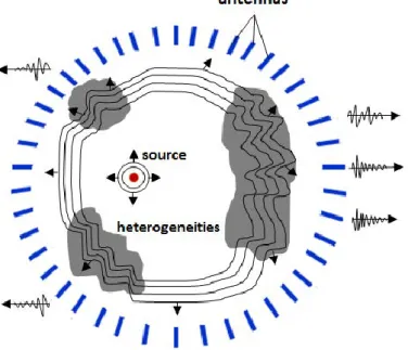
Detection and localization of unknown targets is achieved by placing the object under test in an investigation domain confined by measurement probes which receive parts of the scattered field. Using a classic configuration of a time reversal process, by taking advantage of the spectral degrees of freedom provided by the propagation through a random medium, a microwave imaging method is attained.

The subject of the present thesis is to propose an imaging method in the microwave range by taking advantage of the spectral degrees of freedom provided by the propagation through a random medium. Experimentally, the location of a scatterer can be extracted with a high resolution even though only two antennas are used. The ability to image the target is shown using a synthetic time reversal technique and a matrix inversion method.

This work, supported by the Direction Générale de l’Armement (DGA) was conducted at the Institute d’Electronique et de Télécommunication de Rennes (IETR), with

3

the Compact and Ultra small anTEnnas (CUTE) team of the Antennes et Dispositifs Hyperfréquences department (ADH).

The thesis manuscript is organized in four chapters. The first chapter gives a general description of radar systems and radar cross section basic principles presenting RCS behavior for three types of calibration target, a brief description of the target support structures influence on measurements and the measurement facilities, as well as basic ideas on RCS imagery: one-dimensional range profile/cross-range profile and two-dimensional ISAR image. The second chapter introduces theoretical aspects on time reversal technique, followed by simulations results in FDTD showing the properties of a random medium used in a time reversal process which yields a focus quality that is not dependent on the aperture of the TRM. Using a FDTD method with a PML function to treat the boundaries, 2D simulations are carried out showing also that with multiple sources in a TR process, multiple foci can be obtained on different positions at the same time, or by controlling the distance between the point-like sources a wide focus can be achieved.

The third chapter presents the modeling of a microwave imaging system using a random medium. Conception details regarding the design of the random medium and a few theoretical aspects regarding the characteristics of a random medium used for target detection are given in the beginning. Further it is presented the simulation setup for an imaging method in the microwave range using a random medium. The results are presented for two methods: one based on time reversal technique and another method based on matrix inversion which provides lower sidelobes. As well, inspired from the use of a cavity for microwave imaging, the results of a comparison between simulation setups are presented. Three versions of a chosen simulated setup with different PEC boundaries are compared in order to determine the best results for an imaging method that takes advantage of the spectral degrees of freedom provided by the propagation through a random medium.

The final chapter of the thesis presents the experimental validation of the imaging system using a setup similar with the ones previously presented in simulation, applying both methods based on TR and matrix inversion. Moreover, it is presented a comparison between layouts with an increased number of antennas used to improve the image quality. Comparing the results for the cases of one, two or three antennas used simultaneously, the constructive interferences of their individual contributions, give the best results for the last case.

At the end of the manuscript, are given a general conclusion of the thesis summarizing the obtained results and future work.

5

CHAPTER 1

Radar cross section principles

1.1 Introduction

Radar cross section (RCS) is the measure of an object‟s ability to reflect radar signals in the direction of the radar. It is a measure of the ratio of scattered power density towards the radar to the power density that is intercepted by the target. There are different factors that influence the RCS: the geometry of the target, the materials, the working frequency, the transmitter and receiver polarizations and the directions of the radar transmitter and receiver.

The purpose of this chapter is to present a short overview of radar basic definitions and radar cross section fundamentals, measurement facilities, instrumentation and RCS imagery.

1.2 Radar basic definitions

1.2.1 History of radar

The origins of the basic idea of radar are found in the classical experiments on electromagnetic radiation conducted by the physicist Heinrich Hertz during the late 1880s, when he set out to experimentally verify the earlier theoretical work of the physicist James Clerk Maxwell. By developing the general equations of the electromagnetic field, Maxwell‟s work led to the conclusion that radio waves can be reflected from metallic objects and refracted by a dielectric medium, just as light waves.

Based on the theory demonstrated by Hertz, a first prototype named “Telemobiloskop” was patented in 1904 by Christian Hülsmeyer [1]. The working principle of the device was based on the concept of reflected waves by metallic surfaces. The wave emitted by an antenna, hits a metallic object and is partly reflected back, towards several antennas which were serving as receivers. Hülsmeyer‟s invention did not draw attention since there was no need for the radar until the 1930s when long-range military bombers were developed and brought the interest of detecting the approach of hostile aircrafts.

Radar was developed in the period before and during World War II by several nations: United Kingdom, France, Germany, Italy, Japan, Netherlands, the Soviet Union and the United States. In 1934, following systematics studies, France began developing an obstacle-locating radio apparatus. By the end of the year, the first full radar evolved as a pulsed

6

system, was demonstrated in U.S. The next year, Germany and U.K demonstrated such elementary apparatus.

After the war, the progress in radar technology slowed considerably. The last half of the 1940s was dedicated to developments initiated during the war. Two of these were the monopulse tracking radar and the moving-target indication radar. Many years of development were necessary to bring these radar techniques to full capability.

New and better radar systems emerged during the 1950s, like the high-powered radars designed to operate at 220 MHz and 450 MHz. Being equipped with large mechanically rotating antennas, it could reliably detect aircraft at very long ranges. Synthetic aperture radar first appeared in this decade, but it took almost 30 more years to reach a high state of development.

Furthermore, serious applications of the Doppler principle to radar started to advance becoming vital in the operation of many radar systems. The Doppler frequency shift of the reflected signal resulted from the relative motion between the target and the radar is indispensable in continuous wave and pulse radar, used to detect moving targets in the presence of large clutter echoes.

As the digital age arose in the 1970s, the signal and data processing required for modern radars was made practical. Radar methods evolved over the next decade, to a point where radars were able to distinguish one type of target to another. In the 1990s, due to continued advances in computer technology, increased information about the nature of targets was available [2].

The 21st century brought advances in digital technology which sparked further improvement in signal and data processing with the goal of developing nearly all-digital phased-array radars.

1.2.2 Introduction to radar systems

The term RADAR was conceived in 1940 as an acronym for RAdio Detection and Ranging [3], but later on the term has entered English and other languages as a common noun and lost the capitalization.

As the name implies, radar is an electromagnetic system used for the detection and location of objects such as aircrafts, ships, vehicles or terrain. By transmitting a particular type of wave form, for example a pulse-modulated sine wave, the radar detects a target and

7

from the nature of the echo signal, identifies the distance, range, altitude, direction or speed of the target.

An elementary form of radar consists of a transmitting antenna emitting electromagnetic radiation, a receiving antenna and an energy-detecting device. The target intercepts a part of the transmitted signal and reradiates it in all directions.

The prime interest to the monostatic radar is the energy radiated backwards in the direction of the radar. The receiving antenna collects the returned energy and delivered it to a receiver, where it is processed to detect the presence of the target and to extract its location and relative velocity.

Figure 1.1 presents the working principle of a radar system.

Figure 1.1 Radar working principle

The distance to the target is determined by measuring the time , taken by the signal to travel from the emitting antenna to the target and back. Since electromagnetic waves propagate at the speed of light , the range is expressed:

(1.1)

The direction of the target may be determined from the direction of arrival of the reflected wave-front. The usual method of measuring the direction of arrival is by using narrow beam antennas. To distinguish moving targets from stationary objects, the relative

8

motion between the target and the radar, which is represented in a shift in the carrier frequency of the reflected wave known as Doppler effect, is used as a measure of target‟s relative velocity.

A sufficient length of time must elapse after the transmitted pulse is emitted by the radar, to allow any echo signals to return and be detected before the next pulse may be transmitted. Otherwise, ambiguities in range measurements might result, if echo signals from some targets might arrive after the transmission of the next pulse. Echoes that arrive after the transmission of the next pulse are called second-time-around echoes. Such an echo would appear to be at a much shorter range and could be misleading if it were not known as a second-time-around echo [4].

There are different suitable modulations that can be used. However, the typical radar transmits a simple pulse-modulated waveform. The pulse carrier might be frequency or phase modulated to permit echo signals to be compressed in time after reception, achieving the benefits of high-range resolution without the need to resort to a short pulse. By taking advantage of the Doppler frequency shift to separate the received echo from the transmitted signal and the echoes from the clutter, continuous waveforms (CW) can also be used.

CW radars typically use separate transmit and receive antennas because it is not usually possible to receive with full sensitivity through an antenna while it is transmitting a high power signal [5].

Radars operate in the RF band of the electromagnetic spectrum between 5 MHz and 300 GHz. Table 1.1 lists the radar frequency bands and applications:

Band

Designation Frequency range Wavelength Typical application

HF 3 – 30 MHz 100 – 10 m Observation: over the horizon radar VHF 30 – 300 MHz 10 – 1 m Very long range surveillance _{Ground penetration radar} UHF 300 – 1000 MHz 100 – 30 cm Very long range surveillance _{Foliage penetration} L 1 – 2 GHz 30 – 15 cm Long range surveillance S 2 – 4 GHz 15 – 7.5 cm Medium range surveillance _{Air traffic control} C 4 – 8 GHz 7.5 – 3.75 cm

Long range tracking

Shooting and missile guidance Air traffic control

9 X 8 – 12 GHz 3.75 – 2.5 cm

Combat aircraft radar Short range tracking

Long range ground surveillance Airborne weather radar

Marine radar police radar Ku 12 – 18 GHz 2.5 – 1.67 cm

Guidance

High resolution mapping Airborne altimeter

Medium range ground surveillance K 18 – 27 GHz 1.67 – 1.11 cm Police radar

Ka 27 – 40 GHz 1.11 – 0.75 cm Short range ground surveillance Targeting Imaging

V 40 – 75 GHz 75 – 40 mm Automotive anti-collision W 75 – 110 GHz 40 – 27 mm Imaging Automotive anti-collision

Airborne wire detection mm 110 – 300 GHz 27 – 1 mm Imaging

Table 1.1 Radar frequency bands [6]

Low-frequency radars require large antennas and have limitations on resolution because fine resolution implies large instantaneous bandwidth of the transmit signal. The bandwidth could represent a significant percentage of transmit frequency and may cause problems with the transmitter and receiver design.

1.2.3 Radar equation

The radar equation relates the range of a radar target to the characteristics of the transmitter, receiver, antenna, target and environment, representing a basis for radar design. In monostatic, the received power can be expressed as:

( ) (1.2)

where, is the radar cross section which is a measure of the equivalent or radio-electric size of the target, as seen by the radar, having units of area; is the power radiated by the transmitter; is the gain of the transmitting and receiving antennas; is the wavelength and

is the distance between the radar and the target.

An important use of the radar range equation is the determination of detection range, or the maximum range at which a target has a given probability of being detected by radar.

10

The radar equation can be written under the following form which gives the maximum radar range:

√

( ) (1.3)

where, is the minimum detectable power.

One other form of the basic radar equation takes into account the noise. Considering the bandwidth, of the receiver, the ambient temperature expressed in degrees Kelvin, , and the noise contribution of the receiver, , the noise power at the output can be written as:

(1.4)

where is Boltzman‟s constant.

In this case, the minimum detectable power is expressed as a function of the noise level:

(1.5)

where represents the signal to noise ratio.

Taking into consideration a factor, , representing all the losses, for example from the transmission lines or feeders, the radar range equation becomes:

√

( ) (1.6)

A multitude of factors can degrade radar performance. These factors include those related to radar itself, the environment in which the radar operates the operator of the radar and often, the inexperience of the radar analyst.

1.3 Radar cross section fundamentals

1.3.1 Radar cross section determination

Radar cross section is a measure of the power scattered in a given direction when a target is illuminated by a plane wave. According to IEEE dictionary of standards terms [7], RCS is defined as times the ratio of the power per unit solid angle scattered toward the radar receiver with the power density of the plane wave incident on the scatterer. More

11

precisely, it is the limit of that ratio as the distance from the scatterer to the point where the scattered power is measured, , approaches infinity.

Considering the field incident on the target and , the field scattered by the

target, the radar cross section, is expressed:

| |

| | (1.7)

RCS is a function of multiple parameters, such as: the positions of transmitter and receiver relative to the target, the angular orientation of the target relative to transmitter and receiver, the polarization of transmitter and receiver, the target geometry and material composition and the frequency or wavelength [8].

Three types of RCS are distinguished: a) Monostatic or backscatter RCS when the incident and the scattering directions are coincident but opposite in sense. b) Bistatic RCS when the two directions are different: c) Forward-scatter RCS when the two directions and senses are the same.

Monostatic or backscatter RCS, is the usual case of interest for most radar systems where the receiver and transmitter are colocated, often using the same antenna for transmitting and receiving. Figure 1.2 shows the configuration for monostatic RCS presenting two cases: one with the same antenna used for emission/reception and the second one using two different antennas close enough to be in a monostatic configuration.

a) b)

Figure 1.2 Monostatic radar:

12

Bistatic RCS is the case when the transmitter and the receiver are separated in angle. This configuration is used to express the RCS when the target is illuminated and observed by spatially separated radar stations. Figure 1.3 shows the configuration for bistatic RCS.

Figure 1.3 Bistatic radar

A special case of bistatic radar is the forward scatter radar. Forward RCS is the measure of scattered power in the forward direction, in the same direction as the incident field, as shown in Figure 1.4. This forward scattered power is usually out of phase with the incident field so that when added to the incident field a shadow region is formed behind the scattering object.

Figure 1.4 Forward scatter radar

Modeling software can be used to obtain estimates of target cross sections, but the most accurate method is by measurement, because in this case no approximation is done on the target. However, even this method encounters great difficulty, particularly if the target is large, the far field criteria is not always respected and it is often impractical to measure the cross section over all aspect angles in azimuth and elevation.

The targets are complex and consist of many scattering surfaces. The effective surface roughness of a target, as a function of , plays an important role in determining its RCS.

13

1.4 Scattering regimes

There are three regimes that characterize the RCS scattering, depending on the ratio of wavelength, to the size of the target, ⁄ . In the Rayleigh region, the wavelength is greater than the size of the target, . If the size of the target is comparable with the wavelength , the scattering is in the resonant (Mie) region. The optics region corresponds to wavelengths very small compared to the size of the target, .

Figure 1.5 shows the classic illustration of cross section of a sphere over these three regions. The radar cross section has been normalized to the projected area of the sphere, , plotted as a function of sphere circumference normalized to the wavelength, ⁄ _.

Figure 1.5 Normalized RSC of a metallic sphere over the three scattering regimes

1.4.1 Low-frequency scattering region

Lower frequencies imply greater wavelengths compared with the target‟s body size and the scattering is in the Rayleigh region which is named after Lord Rayleigh. He stated the sky is blue due to the longer blue wavelengths which reach earthbound observers, as opposed to the shorter wavelengths which suffer greater scattering by atmosphere particles.

In the low-frequency case, there is little phase variation of the incident wave over the spatial extent of the scattering body, so each part of the target encounter the same incident

14

field at each moment of time. The situation is similar to a static field problem, with the exception that the incident field is changing in time. This quasi-static field builds up opposite charges at the ends of the body of the target.

When the wavelength is much greater than the sphere circumference, in Rayleigh region, its cross section is proportional to ( ) , where ⁄ _{is the wavenumber.} Consequently, although the radar cross section is small, it increases as the fourth power of frequency and sixth power of radius. The most notable characteristic of Rayleigh scattering is that cross section is proportional to the fourth power of the frequency: .

The strong wavelength dependence means that shorter wavelengths are scattered more efficiently than longer wavelengths [9]. Since Rayleigh scattering is essentially a static field problem, analytical procedures as the integral equation approach or the dipole and multidipole expansions can be invoked.

For low-frequency scattering, the entire body of the target participates in the scattering process. Thus, the details of the shape are not important and only a basic geometric description is required because the overall shape is more significant than detailed shape information.

As the target size increases and becomes comparable to the wavelength, the Rayleigh theory breaks down and Mie theory describes the scattering process.

1.4.2 Mie resonant scattering region

When the incident wave length is on the order of the size of target the phase of the incident field changes significantly over the length of the scattering body. Conventionally, if the size of the target falls between and wavelengths, the scattering is considered to be in the resonant region.

Mie scattering is different from Rayleigh theory by the point of view of the intensity of radiation. Mie-scattered radiation is larger in forward direction than in backward direction and slightly not dependent on the wavelength, while Rayleigh-scattered radiation is identical in forward and backward direction. A distinctive property of Mie scattering, are the Mie resonances, where the scattering is particularly strong or particularly weak [10].

In this region there are two classes of scattering mechanisms, surface wave effects that are unique to only resonant region and the optical mechanism. Surface wave types are traveling waves, creeping waves and edge traveling waves. These waves occur when the

15

surface energy is reflected from some aft body discontinuity, or as in the case for creeping waves, the energy flows completely around the body of the target.

Surface wave scattering is independent of target size. Cross section magnitudes are proportional to ; therefore these effects are important for resonant region target size. Surface wave effects are present in optical region, but the scattering magnitudes are much smaller than optical scattering magnitudes.

In this scattering regime body-body interaction is important as the field at any part of the body is the sum of the incident field and the field scattered by other regions of the target. This collective interaction determines the resultant current density. Overall geometry is important, yet small scale details, compared with the wavelength are not. In this regime an exact solution of Maxwell‟s equations is required. Typically the method of moments is used to solve the integral form of Maxwell‟s equations to obtain the induced currents from which the scattered field is obtained.

1.4.3 High-frequency optical scattering region

When the wavelength becomes much smaller than the size of the target, usually at least ten times smaller, a localized scattering center approach is used. In this region, collective interactions are very weak and the target is treated as a collection of independent scattering centers. In the scattering process, detailed geometries now become important. The net scattering from the target is the complex phasor sum of all the individual scattering centers.

There are several types of scattering mechanism in the optical regime. Specular scattering is the ray optical case of angle of reflection equal to angle of incidence. The scattering is the optical mirror reflection and it is the mechanism responsible for bright spike-like scattering.

The end-region scattering is the scattering from the end regions of finite objects, which produces sidelobe scattering in directions away from specular. Diffraction is end-region scattering in the specular direction due to edge induced currents at leading or trailing edges, tips or object regions of rapid curvature change.

Multiple-bounce is the separate case of mutual body interaction in the sense that one object‟s surface scatters energy to another object surface that is oriented to reflect this energy back to the observer, like corner reflectors or cavities.

16

1.5 Calibration targets

The RCS calibration is the most important part of measurements and a variety of metrological reference targets are considered, such as flat plates, discs, cylinders and corner reflectors in addition to spheres. The flat plate offers the highest RCS for a given size, but it gives a specular reflection which makes it difficult to align.

Another used shape is the trihedral corner-reflector which also produces a high radar cross section which remains constant over a wide angle, being a preferred RCS reference.

The sphere is also often used as a reference for moving targets since its radar cross section is invariant with observed angle. The inconvenient is that the RCS is very small for its size and also large conductive perfect spheres are difficult to manufacture.

It is generally advisable to choose the reference in the upper dynamic range of the measured target. The radar cross section of a sphere is often taken as reference value as the radar return reflected from a target is compared to the one reflected from a sphere. Generally, the accepted size of the sphere circumference has to be 10 times greater than the operating wavelength.

Yet if calibrated, other objects like cylinders, flat plates, dihedral and trihedral corner reflectors or Luneburg lens can also be used for comparative radar cross section measurements [11].

In the next sections, the monostatic RCS of all presented calibration targets have been simulated using CST Microwave Studio 3D EM software. Simulations are carried at central frequency of using a plane wave configuration.

1.5.1 Flat plate

1.5.1.1 Rectangular flat plate

The flat plate is the target which presents the largest peak RCS for its size [12]. Its echo near normal incidence is known with a high degree of confidence.

Generally, the flat plate is used as reference target when it is observed at normal incidence, where the monostatic RCS of a rectangular plate becomes:

(1.8)

17

As an example, a square plate is modeled in CST MWS 3D EM using a perfect electrical conductor (PEC) as the material. The sides of the plate have the dimension equal to five wavelengths, , for the central frequency of . Figure 1.6 presents the square plate.

Figure 1.6 Square plate

The monostatic RCS as a function of aspect angles of a PEC plate, shown in Figure 1.7, is simulated facing a plane wave.

Figure 1.7 Simulated monostatic RCS of a flat square plate

Because the sidelobes of this pattern are governed by a function, the first sidelobes are lower from the normal-incidence echo of the square plate.

1.5.1.2 Circular flat plate

For a circular flat plate, the normal-incidence RCS is also high, but its sidelobes decay faster away from normal incidence in comparison with the square flat plate. For normal incidence, the monostatic RCS of a circular plate is expressed as:

(1.9) -90 -70 -50 -30 -10 10 30 50 70 90 -30 -20 -10 0 10 20

Aspect angle, degrees

R C S, d Bm 2

18 where, is the radius of the plate.

For instance, a PEC modeled circular plate with a diameter equal to five wavelengths, , shown in Figure 1.8, has the simulated monostatic RCS at presented in Figure 1.9.

Figure 1.8 Circular plate

The normal-incidence value for the circular flat plate is lower than that of the circumscribing square plate due to the area reduction from the square shape to the circular one, especially near the sides of the disc.

Figure 1.9 Simulated monostatic RCS of a flat circular plate

In this case the first sidelobe level is below the normal incidence echo, while the first sidelobe level for the square plate is below the normal incidence echo.

1.5.2 Dihedral reflector

The dihedral corner reflector consists of two faces joined at right angles. Even if the faces may have different shapes, the dihedrals used for calibration have rectangular faces. Among the passive reflectors, the dihedral corner reflector is most suitable for polarimetric calibration measurements [13]. -90 -70 -50 -30 -10 10 30 50 70 90 -30 -20 -10 0 10

Aspect angle, degrees

R C S, d Bm 2

19

The studied reflector is a PEC modeled rectangular dihedral reflector whose square faces have the dimension of . Figure 1.10 presents a rectangular dihedral reflector with .

Figure 1.10 Dihedral reflector

Figure 1.11 shows the monostatic RCS of the square-faced dihedral corner reflector presented in Figure 1.10, illuminated by a plane wave at the frequency of .

Figure 1.11 Simulated monostatic RCS of a dihedral reflector

The dihedral reflector has a similar scattering mechanism as the metal plate [14]. The dominant echo mechanism is a double bounce, one per face. The echo reaches its peak when the corner is seen from a direction along the bisector of the corner angle and in a plane perpendicular to the dihedral axis.

The ripples in the pattern are due to sidelobes of the single bounce flat-plate returns, combined with the double-bounce interaction between two faces [15]. The first bigger sidelobes are the main lobes of the single-bounce patterns.

-90 -70 -50 -30 -10 10 30 50 70 90 -30 -20 -10 0 10 20

Aspect angle, degrees

R C S, d Bm 2

20

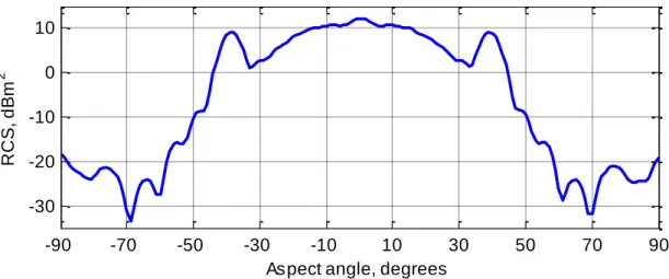
1.5.3 Trihedral reflector

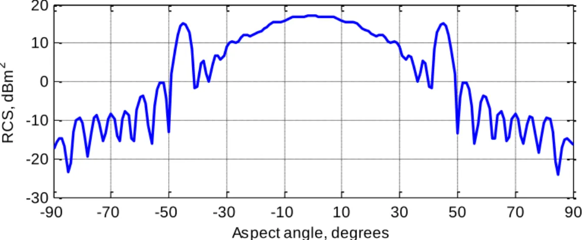
The typical trihedral reflector consists of three flat plates mutually orthogonal joined in a corner where the dominant scattering mechanism is a triple bounce in which all three faces of the trihedral participate. The common shapes of the plates are squares, quarter-discs or right triangles.

1.5.3.1 Rectangular trihedral reflector

One type of trihedral corner is the rectangular three-face reflector. As an example, a PEC modeled reflector consisting of three square plates is considered. The sides equal to five wavelengths, . Figure 1.12 presents the trihedral rectangular reflector.

Figure 1.12 Rectangular trihedral reflector

The RCS for normal incidence to the corner aperture is expressed as [16]:

(1.10)

Figure 1.13 shows the monostatic RCS of the three-faced rectangular trihedral reflector, illuminated by a plane wave at the frequency of .

Figure 1.13 Simulated monostatic RCS of a rectangular trihedral reflector

-90 -70 -50 -30 -10 10 30 50 70 90 -30 -20 -10 0 10 20

Aspect angle, degrees

R C S, d Bm 2