Species responses to climate change and landscape fragmentation: the central role of dispersal

(1)

THÈSE

En vue de l’obtention du

DOCTORAT DE L’UNIVERSITÉ DE

TOULOUSE

Délivré par : l’Université Toulouse 3 Paul Sabatier (UT3 Paul Sabatier)

Présentée et soutenue le 12/03/2019 par :

Félix Pellerin

Species responses to climate change and landscape

fragmentation: the central role of dispersal

JURY

François Massol Directeur de recherche Rapporteur

Donald B. Miles Professeur d’université Rapporteur

Aurélie Coulon Chargée de recherche Examinatrice

Nicolas Schtickzelle Professeur d’université Examinateur

Jean-Louis Hemptinne Professeur d’université Directeur

Julien Cote Chargé de recherche Directeur

Robin Aguilée Maître de conférence Directeur

École doctorale et spécialité :

SEVAB : Écologie, biodiversité et évolution

Unité de Recherche :

Évolution et Diversité Biologique, UMR UPS-CNRS-IRD, Toulouse

Directeur(s) de Thèse :

Jean-Louis Hemptinne, Julien Cote et Robin Aguilée

Rapporteurs :

(2)

(3)

Remerciements

Je tiens par commencer à remercier les deux rapporteurs de ce travail de thèse, François Massol et Donald Miles qui ont accepté de relire et d’évaluer ce manuscrit. Je remercie également Aurélie Coulon et Nicolas Shtickzelle d’avoir accepté de faire parti de mon jury en tant qu’examinatrice et examinateur. Merci également aux membres de mon comité de thèse, Ophélie Ronce, Sandrine Meylan et Emanuel Fronhofer pour les conseils avisés qu’ils m’ont fournit et le temps qu’ils m’ont accordé au cours de mes deux (très longs) comités.

Je tiens ensuite à remercier de tout mon cœur mes directeurs de thèse qui m’ont supporté pendant ces trois années. Tout d’abord, merci Robin Aguilée. Je commence par toi, car c’est toi qui m’a ouvert les portes de la recherche et d’EDB pour la première fois, au cours de mon stage de M1. Je pense qu’il n’est pas nécessaire de préciser que j’aime vraiment bien travailler avec toi, puisque je ne te quitte plus depuis 5 ans maintenant. Merci de m’avoir inculqué la rigueur scientifique et le gout pour la programmation. Merci également d’avoir essayé de me transmettre ton niveau d’organisation hors norme. Bon visiblement ça n’a pas trop bien marché, rien qu’à voir l’état de mon bureau. Mais je te promets, je fais quand même des efforts (j’ai quand même la place de poser mon ordi directement sur le bureau, sans feuille de brouillon, peau de clémentine ou coquille de noix dessous ! !). Merci également pour les à cotés de la thèse, les sorties vélos, les sorties ski de rando et bientôt j’espère les sorties escalades ! !

Merci ensuite à Julien Cote. Je crois que j’aurais passé plus de temps avec toi durant ces trois dernières années, qu’avec quiconque d’autre. Merci de m’avoir tout appris de l’écologie expérimentale, des lézards vivipares et des statistiques. Merci de m’avoir fait confiance en M2 puis en thèse. Merci d’avoir été toujours présent, sur le terrain comme

(4)

en dehors. Merci aussi pour les bons petits plats (surtout la carbonade flamande) et les verres de gnole. Merci pour les « ça va aller » alors que t’étais deux fois plus stressé que moi. Merci pour le k-way rose au crabère. J’ai vraiment apprécié travailler à tes cotés. Je mesure la chance que j’ai eu d’avoir un directeur de thèse comme toi, qui est venu à chaque fois sur le terrain avec moi, et ça je crois que très peu de thésard peuvent s’en vanter. Donc merci beaucoup pour tout ça. Je cois de toute façon qu’on va encore rester en contact un bon moment, vu la quantité de données qu’il reste à analyser et de papiers à publier.

Dans la famille des directeurs de thèse, je tiens finalement à remercier Jean-Louis Hemptinne. Prévu initialement pour quelque mois, puis finalement jusqu’au bout, merci beaucoup d’avoir accepté de t’associer à cette thèse. Merci pour ton sourire bienveillant et ton calme rassurant. Et surtout, merci de diriger de laboratoire comme tu le fais. Merci de parfois le tenir à bout de bras et de continuer malgré les écueils. Les thésards d’EDB s’associent pour te faire un câlin géant !

Mes remerciements vont ensuite tout naturellement à mes collègues de terrain, Laurane Winandy, Lucie Dy gesu et Elvire Bestion.

Merci Elvire, pour tout et plus encore. Tu as été parfaite en M2 et parfaite en thèse que ce soit à distance ou sur le terrain cette année. Merci d’avoir mis en place la base de données (bon, pour le nombre de colonnes, on a encore un petit effort à faire, et peut être sur certain noms de colonne aussi), merci d’avoir mis en place tous les protocoles pendant ta thèse, je crois que sans ça je n’aurais rien pu faire. Merci pour les relectures de papier, merci pour tes captures hors normes (même si pour faire plaisir à Julien on va dire que c’est lui qui gagne ;)), merci pour tes connaissances en stat et enfin merci pour ton efficacité redoutable dans à peu près tout ce que tu entreprends. Mais aussi merci pour les petits fou rire qu’on s’est pris sur le terrain (je me rappel d’un beau lors de la randomisation des terrariums. . . .), les carrés de chocolat et les cours de grammaire espagnol ! !

Merci Laurane pour ta compagnie et ton soutien pendant ces trois années de thèse. Je crois que sans toi, ça n’aurait pas eu la même saveur. Merci pour ces trois années de

(5)

terrain pendant lesquelles tu m’as épaulé sur toutes les manips, merci pour les 11 semaines d’émergence et les 8 jours de performance thermique, merci pour les craquages de fatigue, merci pour les rosaces et les chansons de merde, merci pour ton accent et tes expressions, merci pour ton deuxième prénom, merci pour les bières belges et les blagues salasses, merci pour les rando et les aprem à glander et surtout merci pour ta complicité. Enfin bref merci pour tout Sergio, on se sera quand même bien marré et j’espère bien que ce n’est que le début ! !

Merci Lucie pour ton aide précieuse pendant les deux premières années de terrain, merci de m’avoir tout appris de l’élevage et du metatron, merci pour les fichiers globaux et le tri des insectes ! ! Merci aussi pour les grandes discussions sur nos futures vies, merci pour les pauses gouté, merci pour tes plats de pates et tes furets, merci pour ton calme légendaire. Merci d’avoir râlé et d’avoir bougonné, ça m’aura bien fait rire. Et même si je pense t’avoir tapé sur le système un bon petit nombre de fois, tu ne m’as jamais vraiment envoyé chier (ou alors t’as essayé mais c’était trop subtile et je n’ai pas compris) et ça c’est bien gentil de ta part.

Je tiens ensuite à remercier tous les étudiants que j’ai eu le plaisir d’encadrer pendant cette thèse et sans qui il nous aurait été impossible de faire ces expériences. Un grand merci donc à Quentin Salmon, Eléonore Rolland, Pierre Tardieu, Mickael Baumann, Manon Bincteux, Anabella Heintz, Rebecca Loiseleur, Audrey Gourmand, Igor Boyer, Emilie Levesque, Naomi Jallon, Lucile Rabardelle, Maxime Aubourg, Bérénice Givord-Coupeau, Audrey Bourdin et Jules Brochon. Vous avez tous été super !

Un grand merci à Murielle Richard pour toutes les extractions, toutes les lectures de pics et toutes les analyses de paternités ! ! Vraiment, merci pour tout ça, je sais que ce n’est pas toujours passionnant et qu’on te laisse parfois un peu seule. Mais grâce à toi on va pouvoir faire des super analyses ! ! Merci beaucoup aussi pour ta participation à mes comités de thèse et les discussions qu’on a pu avoir autour des questions de génétique et de lézard ! ! Merci également à Olivier Guillaume et Thomas Deruelles pour le soutien technique et logistique au Métatron. Un énorme merci à Guillaume Toumi pour tous les travaux que tu as fait au Métatron. Merci pour le Karcher et les réparations ! ! Et merci

(6)

pour ta disponibilité et ta persévérance ! ! !

Merci ensuite au pole administratif et financiers du laboratoire EDB et de la SETE de Moulis. Je tiens à remercier particulièrement Catherine pour les ordres de mission et les commandes de grillons ! ! Merci également à l’école doctorale SEVAB de m’avoir accordé cette bourse de thèse. Un grand merci à Dominique pour ton professionnalisme, ta gentillesse et ta capacité à avoir détecté au premier coup d’œil ma phobie administrative ! Vient maintenant le tour des collègues de bureau ! ! Je crois que c’est quand même le plus important. Je me vois dans l’obligation de commencer par Jessou d’escalquens. Merci Jessou pour les heures passées à se marrer. On n’aura peut être pas révolutionné la science mais on aura bien rigolé ! Donc même si tu passes plus de temps à dire que tu vas au sport qu’à réellement y aller, on aura bien bossé les abdos. Merci pour tout Jessou, je suis très très content d’avoir perdu à la courte paille contre Marine et de m’être retrouvé dans ton bureau ;). Merci aussi pour les discussions sérieuses (oui, il y a eu parfois) et les questions de génèt quanti, tout ça sur un air d’Eddy Mitchell (« oh danielo. . . »). Un grand merci aussi à Magdalena pour ton calme et ta gentillesse, et aussi de nous avoir supporté avec Jessica sans jamais broncher. Merci aussi à Guillhem en début de thèse, à Sandra ensuite et finalement à E Ping. Famille bureau 18 forever ! ! Enfin, merci à Josselino, fondateur de la lignée 18 et qui n’a jamais vraiment quitté le bureau ! j’espère avoir été à la hauteur du bureau près de la fenêtre ! !

Merci ensuite à mes compagnons de cordé, mes conscrits de promo, mes coéquipiers d’aventure. Je veux bien sur parler de Marine et de Seb ! ! ! Marine, merci pour ces 3 années, sans toi je n’aurai pas survécu ! il y aurait trop de choses à dire alors je vais faire une sélection : merci pour les soirées endiablées, merci pour claude nougaro, merci pour les coupes à la Godefroy de Montmirail, merci pour toutes tes maladresses, merci pour tes calins, merci pour les randos, merci pour l’escalade, merci pour Amsterdam, merci pour le chouchen, merci pour ta complicité, merci. . . . J’espère que ça va encore continuer un bon nombre d’année parce que je ne pense pas pouvoir me lasser/passer de toi. Evidemment, la suite de ce paragraphe concerne le troisième mousquetaire, Sebou de la jungle. Merci Seb d’exister ! Merci pour ton cœur tendre sous tes kilos de muscle. Merci pour ton humour et

(7)

ton premier degré. Merci pour les randos et ton sens de l’organisation ! merci pour les fruits séchés et les kiwis avec la peau. Merci pour tes shorts en hiver et ton pull seb 18. Merci pour notre fin de thèse commune et nos plans sur la comète à 20h30 dans ton bureau. Merci pour tout Seb, t’es vraiment un mec génial ! J’attends les prochaines escapades en montagne avec impatience, les bivouacs sur les cimes, les brames du cerf sous la pluie, les levers de soleil sur les sommets enneigés. Bref, j’attends qu’on reprenne nos discussions sur la vie autre part qu’au 4R1. Et si tu n’as toujours pas compris, c’est un appel du pied pour qu’on s’organise une petite virée nature ensemble dans les prochains mois ! !

Mes remerciements vont ensuite à Kevin Cilleros. Kevin, merci pour toutes les réponses à mes questions, merci pour les fractales et surtout merci pour le chocolat ! ! Merci aussi Jade pour les randos et le soutient moral apporté. Merci Lucie pour les beer party et tes histoires de cœurs. Merci Isou pour tes pulls tachés et ton humanité débordante. Merci Alexou pour les pintes de guiness et tes pieds du 56. Merci Juanito pour les discussions sur le canap du bureau 33 et ton rire discret. Merci Luana pour les sauts de biche et les cours IPE, merci glanlan pour ton parasitisme légendaire, tes parties de rockfoot endiablées, ta descente du crabère et la salade de riz. Merci Céline pour les TP de L1 et les expressions outrées. Merci Maxou pour ton humour à tomber et tes répliques d’OSS117. Merci Maeva pour les sorties bota et ton micro sac en rando. Merci MC Jordi, Nico et Lionel. Merci Fabian pour tes jeux de mots et tes tapes dans le dos (parce que ça rime). Merci Iris pour tes talents de musicienne. Merci Jan pour ton humour pince sans rire et tes siestes obligatoires. Merci Mathilde pour les sessions slack, les massages crâniens et quelques phrases mémorables. Merci Guillaume pour les « alors la thèse, ça avance ? ». Merci Pierrick pour toutes les inspirations à voyager, les soirées vin fromages, le ramassage d’ordure et ton amitié. A Moulis, merci Jonathan pour les soirées au gite, les sorties en montagne et les blocs du pan. Merci Keoni pour les cueillettes de champignon, les pèches fantastique d’écrevisse, ton souffle et les concerts de gonfleur. Merci Aisha pour les soirées à l’hébergement, terre de couleur et la relecture de mon papier. Merci Léa pour ton soutien de fin thèse, on en aura passé des dimanches tout les deux en salle thésard. Merci Allan pour les sorties vélo et ta clés de la salle chimie (j’avoue, je te l’ai emprunté quelques fois).

(8)

Merci Jérémie pour tes bien bonnes et ton animation de la salle thésard. Merci Lisa pour ton rire et vive le limousin ! ! Merci Staffan pour les quelques semaines de manip tetra, on en aura quand même un peu chié. Merci Delphine pour les bonbons ! ! Merci Mimi pour les conseils avisés.

Merci également aux personnes extérieures à la recherche pour leur soutient pendant ces trois années de thèse. Merci à ma famille et à mes amis de Toulouse et d’ailleurs. Merci Adrien pour les soirées Depardieu/vin rouge et les dizaines de conneries racontées. Merci Laure, PH, Jérémy, Kéké, Toto, Marie, Mathurin, Quentin, Thibaud, Mélusine, Jeanne, Colin, Jérémie. Merci Christian, Maryse et Gabi. Et pour finir, un immense merci Marisa pour ton soutien sans faille la dernière année de thèse, pour m’avoir remotivé quand j’en avais besoin, pour ta semaine de vacance sacrifiée, pour le yaourt Oikos, pour toutes les petites et les grandes attentions et pour m’avoir permis d’avoir amélioré mon niveau d’anglais ;). Obrigado por tudo e pelos restantes 49 anos !

(9)

1 General Introduction

1 Climate change and landscape fragmentation:

evi-dence and consequences for biodiversity

The climate is undoubtedly changing at an accelerated pace worldwide. The Inter-governmental Panel on Climate Change, in their fifth assessment report (IPCC, 2014), summarized the different components of climate change, their evidence, and their links

with human activities. Global earth surface temperature showed a 0.85◦C increase

be-tween 1880 and 2012. Moreover, the last 30 years (1983-2012) was the warmest period (90-100% of likelihood) over the last 800 years. The frequency of extreme events such as extreme warm temperature and extreme precipitation also increased in recent decades (IPCC, 2014). Global warming trends are predicted to be at least maintained or even exacerbated in the next century due to the increase in human induced greenhouse gas emissions (Santer et al., 2013). Depending on the socio-economic contexts, models

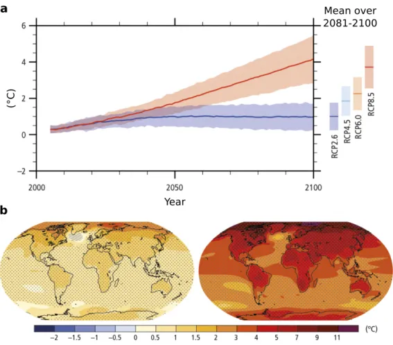
pre-dict an increase in average surface temperature of 1.0 to 3.7◦C in 2081-2100 relative to

the 1986-2005 period (Figure 1.1, Table 1.1). Increasing temperatures are predicted to be associated with higher and longer extreme warm temperature events, a change in the water cycle and an increase in sea level. Past and future climate change affect human and natural systems in return, making climate change one of the main causes of biodiversity changes observed nowadays (Brooks et al., 2002; Parmesan, 2006; Selwood et al., 2015).

(14)

(Parme-Mean over 2081-2100 (°C) Year a b

Figure 1.1 – Change in average global air temperature depending on different socio-economic scenarios (IPCC, 2014). (a) Global average surface temperature change from

2006 to 2100 relative to 1986–2005. (b) Change in average surface temperature for

2081–2100 relative to 1986–2005 under the RCP2.6 (left) and RCP8.5 (right) scenarios. Figure reconstructed from IPCC (2014).

Scenario 2046 - 2065 2081 - 2100

RCP2.6 1.0 [0.4-1.6] 1.0 [0.3-1.7]

RCP4.5 1.4 [0.9-2.0] 1.8 [1.1-2.6]

RCP6.0 1.3 [0.8-1.8] 2.2 [1.4-3.1]

RCP8.5 2.0 [1.4-2.6] 3.7 [2.6-4.8]

Table 1.1 – Projected change in global mean surface temperature (and 5 to 95% model range predictions) for the mid- and late 21st century, relative to the 1986–2005 period. Table reconstucted from IPCC (2014)

san, 2006; Selwood et al., 2015; Urban, 2015, 2018). Both abiotic and biotic factors could lead populations to go extinct under climate change (Cahill et al., 2013). Warming climate should indeed make temperature exceed thermal tolerances of most organisms (Deutsch

et al., 2008; Sinervo et al., 2010). It could result in individual death due to

(15)

refuge to avoid overheating. However, the time spent into refuge limits time dedicated to other vital activities such as foraging. As a consequence, restriction in periods of activ-ity could hamper major physiological functions (metabolism, growth rate, reproduction) and increase extinction risk (Sinervo et al., 2010). Moreover, climate change can modify biotic interactions; for instance it could disrupt mutualistic interactions (Memmott et al., 2007), promote competition and/or pathogens (Pounds et al., 2006) and have a negative impact on beneficial species such as decreasing the amount of prey for a predator species (Memmott et al., 2007). Even if evidence remains relatively scarce (Cahill et al., 2013), population extinction has already been observed (Parmesan et al., 1999; Wilson et al., 2005; Pounds et al., 2006; Thomas et al., 2006; Pacifici et al., 2017; Urban, 2018). Models forecasting future species distribution under climate change predicted the extinction of 5 to 37% of all species depending on the geographic location (Thomas et al., 2004; Urban, 2015). Furthermore, these models predicted impacts of climate change on biodiversity without considering other elements of global change which may act in synergy with cli-mate change (Opdam & Wascher, 2004; Brook et al., 2008; Bellard et al., 2015). Global change refers to changes in the earth system and encompasses changes in climate, land cover, pollution, sea level, urbanization, ocean cycles, carbon cycles. . . . Global change is commonly used to refer to changes associated with human activities (e.g. climate change, pollution, landscape fragmentation). Among them, landscape fragmentation is predicted to be the main threat to biodiversity in terrestrial area (Sala et al., 2000; Jantz et al., 2015).

Agriculture, deforestation and urbanization change the landscape structure. Impor-tant amount of natural habitats are lost and the remnant parts are split in small and isolated patches (i.e. landscape fragmentation, Wilcove et al., 1986; Fahrig, 2003). Land-scape fragmentation often gathers habitat loss (i.e. loss of sustainable habitat) and habi-tat fragmenhabi-tation per se (i.e. the "breaking apart" of habihabi-tat independently of habihabi-tat loss; Fahrig, 2003). Landscape fragmentation impacts biodiversity by reducing patch size, increasing isolation and edge effects and altering patch shapes and matrix structure (Did-ham, 2010). Whereas habitat loss has a strong negative effect on biodiversity (e.g. Brook

(16)

et al., 2003), habitat fragmentation per se can have either positive or negative effects on

biodiversity (Fahrig, 2017). For instance, reducing patch size decreases the number of species present in a given habitat (species-area relationship, e.g. Seabloom et al., 2002). Habitat fragmentation per se also increases the proportion of edges for a given amount of habitat. Edges could increase population extinction as it promotes emigration of in-dividuals into the unsuitable matrix (Fahrig, 2003). On the other hand, edges could be advantageous for particular species preferring warmer and drier conditions (Fahrig, 2003; Didham, 2010). Overall, habitat loss and fragmentation have been shown to reduce biodiversity by 13 to 75% (Haddad et al., 2015) and could have a long lasting effect on future species persistence (i.e. extinction debt, Tilman et al., 1994; Debinski & Holt, 2000; Krauss et al., 2010; Dullinger et al., 2012). Moreover, models predict further extinction due to the increase in fragmentation related to human activities (Pereira et al., 2010; Jantz et al., 2015).

Contemporary global change encompasses major threats to biodiversity. The different factors constituting global change act on their own and in synergy to affect populations, species, communities and ecosystem structure and functioning (Warren et al., 2001; Op-dam & Wascher, 2004; Jetz et al., 2007; Brook et al., 2008; Hof et al., 2011; Comte et al., 2016; Pereira et al., 2010). For instance, Hof et al. (2011) projected the three major threats to amphibian diversity worldwide (climate change, landscape fragmentation and pathogens) and noticed that the different threats often co-occurred, making prediction re-garding threats taken independently irrelevant. Moreover, the different drivers of species extinction often interact. For example, population decline of a rotifer species under ex-perimental conditions was 50 times faster when different threats acted in synergy rather than independently (Mora et al., 2007). Amphibian extinction in Costa Rica was also due to synergetic effects of different threats. Climate change is threatening amphibians on its own by increasing risk of overheat and desiccation. Moreover, climate change is also promoting a pathogen (Batrachochytrium), surging species extinction in this region (Pounds et al., 2006). The different drivers of global change could also act in opposite di-rections. In the cooler part of their range, climate change could be beneficial for species.

(17)

However, landscape fragmentation could buffer or reverse the positive effect of climate change. Warren et al. (2001) observed a strong population decline of many butterfly species in the northern part of their range, where climate change was predicted to be beneficial, because of landscape fragmentation.

Landscape fragmentation could also buffer species responses to climate change (e.g. Opdam & Wascher, 2004). Species are indeed able to respond to climate change (i.e. range shift, phenotypic changes) through different mechanisms. These responses could buffer the effect of climate change on biodiversity. Nevertheless, landscape fragmentation might affect these responses and either limit or hamper species response to climate change (Warren et al., 2001; Opdam & Wascher, 2004). A better understanding of how climate change and landscape fragmentation interact to shape future species distribution and composition is therefore one of the current major scientific challenges in ecology (Selwood

et al., 2015).

2 Responses to climate change in a fragmented

land-scape

2.1 Range shift and phenotypic changes

Two non exclusive responses may allow species to persist under climate change: range shift, and population phenotypic changes. Individuals can first follow through space the suitable climatic conditions, resulting in a change in the spatial distribution of populations (Parmesan & Yohe, 2003). Latitudinal and altitudinal shifts in response to climate change have been already recorded in different taxonomic groups (e.g. insects (Parmesan et al., 1999), plants (Kelly & Goulden, 2008), fishes (Perry et al., 2005)). Chen et al. (2011) measured that species are currently moving on average at a rate of 11 meters per decade in altitude and 16.9 kilometres in latitude in response to climate change. However, there is a strong variation among species in their rate of shift (Chen et al., 2011; MacLean & Beissinger, 2017). Species traits could indeed modulate species range shifts under climate

(18)

change (Angert et al., 2011; MacLean & Beissinger, 2017). Traits might shape the ability of individuals to colonize new habitats at the cold margin of the species distribution (Perry et al., 2005; Pearson, 2006; Angert et al., 2011; Schloss et al., 2012; MacLean & Beissinger, 2017). For example, Schloss et al. (2012) predicted that 9.2 to 39% of mammal species may be unable to track suitable climatic conditions due to dispersal limitation in the northern hemisphere. However, as the different responses to climate change are non-exclusive, trait distributions could also change in response to climate change, and affect species range shift (Figure 1.2).

Populations could indeed respond to climate warming by changing their phenotypic composition without shifting their geographical range (Parmesan, 2006; Lavergne et al., 2010). One of the main phenotypic changes observed in response to recent climate warm-ing was phenological shift (Parmesan & Yohe, 2003; Réale et al., 2003; Root et al., 2003; Menzel et al., 2006; Charmantier et al., 2008; Massot et al., 2017). Individuals advanced their spring events (e.g. breeding, laying date, flowering, budbursting) with increasing spring temperature (Parmesan & Yohe, 2003). Other phenotypic change, such as change in melanism (Roulin, 2014; MacLean et al., 2019), body size (Daufresne et al., 2009; Gardner et al., 2011; Sheridan & Bickford, 2011), morphotype (Gibbs & Karraker, 2006) and physiology (Seebacher et al., 2015) were also linked to climate change. In particu-lar, climate change effects on life-history traits (i.e. survival, growth, reproduction and dispersal) could have important impacts on species responses to climate change as they re-sult in change in population dynamics (Whitfield et al., 2007; Ozgul et al., 2010; Bestion

et al., 2015b). Climate-dependent population dynamics have been studied in different

taxonomic groups (e.g. insects (Deutsch et al., 2008), birds (Jenouvrier et al., 2018), mammals (Ozgul et al., 2010), reptiles (Le Galliard et al., 2010)) and encompass changes in population density, age and size structure (Whitfield et al., 2007; Daufresne et al., 2009; Cunningham et al., 2017). For instance, climate change affects population size structure and/or age structure in ectotherms toward smaller and younger individuals (Daufresne

et al., 2009; Gardner et al., 2011; Sheridan & Bickford, 2011). In fish populations,

(19)

negative effects on the survival of bigger individuals, affecting population size structure (Vindenes et al., 2014). Change in life-history traits also influences demography by deter-mining population density. As evolutionary and demographic processes are closely linked (i.e. eco-evolutionary dynamics (Le Galliard et al., 2005a; Kokko & López-Sepulcre, 2007; Schoener, 2011)), population density could affect the phenotypic response of population to climate change (Figure 1.2). For instance a decrease in population density could in-crease the strength of genetic drift, reduce the efficiency of selection, and lead to the fixation of deleterious mutations in the population. As a result, mean population fit-ness should be reduced, leading to further reductions in population size (Legrand et al., 2017). Changes in population dynamics could therefore affect the relative influence of the processes behind population phenotypic changes, namely phenotypic plasticity and evolutionary adaptation.

Phenotypic plasticity is the ability of a genotype to produce different phenotypes in different environments (Pigliucci, 2001, 2005). Plasticity could thus modify population phenotypic distribution without any change in allele frequencies. Climate driven pheno-typic changes due to phenopheno-typic plasticity have been observed in many studies (reviewed by Boutin & Lane, 2014; Charmantier & Gienapp, 2014; Crozier & Hutchings, 2014; Franks et al., 2014; Reusch, 2014; Schilthuizen & Kellermann, 2014; Stoks et al., 2014; Urban et al., 2014). For example, great tit populations in the UK plastically advanced their laying date in response to warmer spring temperature (Charmantier et al., 2008). Plasticity allows a fast response to environmental changes. However, the range of phe-notype which can be produced by plasticity is not infinite. Moreover, plasticity could be costly to develop (DeWitt et al., 1998). Plasticity could therefore fail to continuously produce phenotypes able to cope with continuously changing environment (DeWitt et al., 1998). Furthermore, climate change could modify the link between reaction norm and fitness, making initially adaptive plastic changes maladaptive (Visser, 2008; Charmantier & Gienapp, 2014). For instance, breeding time in bird could be influenced by temperature as temperature determined the period of higher abundance of caterpillar for their chicks. However, if the correlation between caterpillar abundance and temperature is modified,

(20)

plastic response of bird to temperature will become maladaptive (Visser, 2008).

Evolutionary adaptation affects population phenotypic distribution through changes in allele frequencies. Under climate change, some genotypes produce phenotypes better adapted than others to the new climatic conditions and should be favored by natural selection. Evolutionary adaptation could be fast enough to play a role in population re-sponses to contemporary climate change. For example evolutionary adaptation accounted for 13% of the advance in the breeding timing of Canadian populations of red squirrels in response to increasing spring temperature (Réale et al., 2003). The capacity of a popula-tion to respond to climate change though evolupopula-tionary adaptapopula-tion should depend on its genetic diversity; the higher the genetic diversity, the higher the probability for an allele adapted to the new climatic conditions to be present. Population density could also play a central role as it will determine the strength of genetic drift that could hinder evolution-ary adaptation, and the probability for a new mutation to appear. Phenotypic plasticity could also affect (positively or negatively) evolutionary adaptation (Crispo, 2008).

Phenotypic plasticity and evolutionary adaptation are indeed closely related (Fig-ure 1.2). Historically, phenotypic plasticity was thought to hinder evolutionary adapta-tion by buffering the selective pressures able to select optimum genotypes (DeWitt et al., 1998). However, phenotypic plasticity has been demonstrated to promote evolutionary adaptation (e.g. Price et al., 2003). Plasticity could indeed allow individuals to fast adapt to a new environmental condition and then evolutionary adaptation could replace phe-notypic plasticity, for instance, if plasticity is costly to maintained (Conover & Schultz, 1995). Phenotypic plasticity can also be maladaptive and bring phenotypes to the wrong direction regarding the environmental conditions. In this case, evolutionary adaptation could be favored. Evolutionary adaptation could also directly act on phenotypic plastic-ity. Phenotypic plasticity has been demonstrated to be heritable and susceptible to evolve (Scheiner, 1993; Pigliucci, 2005; Crispo et al., 2010). Evolutionary adaptation could thus favor or hinder phenotypic plasticity depending on the costs associated with plasticity (DeWitt et al., 1998), the spatio-temporal variability in the climatic conditions and if plasticity is adaptive or maladaptive (Crispo, 2008; Crispo et al., 2010; Gibbin et al.,

(21)

2017). The link between plasticity and evolutionary adaptation could also be shaped by dispersal and gene flow (Figure 1.2). Among its effects on species responses to climate change (see below), dispersal could indeed affect the genetic composition of populations, modifying the potential for evolutionary adaptation, and favor phenotypic plasticity as dispersers susceptible to persist under different environmental conditions will be advan-taged (Sultan & Spencer, 2002).

2.2 Central role of dispersal in species response to climate change

Dispersal, the movement of individuals from birth site to breeding site or between two breeding sites (Howard, 1960), plays a central role in species response to climate change. Dispersal affects both range shift and population phenotypic change (Figure 1.2). Dis-persal allows the colonization of new habitat made available by climate change, and thus species range shift. Dispersal also induces a gene flow among populations which can fur-ther modulate the evolutionary adaptation to climate change (Figure 1.2, Lavergne et al. (2010)). Individuals arriving into a population could bring either adaptive or maladaptive genes, promoting and swamping local adaptation respectively (Lenormand, 2002). Theory predicts that the swamping effect of dispersal from core populations to margin populations could limit species distribution (Bridle & Vines, 2007), and could compromise persistence under climate change (Pease et al., 1989; Polechová et al., 2009). More precisely, dispersal could either accelerate the phenotypic shift toward phenotypes better adapted to warmer conditions by bringing pre-adapted genotypes (at the cold margin mostly) or limit adap-tation through a continuous flow of maladapted individuals (at the warm margin mostly). At a finer scale, gene flow among populations inhabiting different microclimates could affect metapopulation dynamics and compositions. Dispersal affects population density and its link to evolutionary processes (Figure 1.2). Moreover, whereas climate warming is not homogeneous through the landscape (Ashcroft et al., 2009), habitats less affected by climate warming may act as source populations allowing the rescue of nearly extinct populations through dispersal (Pearson, 2006; Hannah et al., 2014; Lembrechts et al., 2018). Conversely, less affected populations may limit population adaptation to warmer

(22)

conditions by continuously sending maladaptive genes into the most affected populations. As already mentioned at the end of the previous section, dispersal could modulate the link between evolutionary adaptation and phenotypic plasticity (Figure 1.2). Dispersal should shape the relative importance of evolutionary adaptation and phenotypic plastic-ity in population phenotypic changes in response to climate change. First, by allowing spatial range shift, dispersal could hamper selective pressures on phenotypes and help catch up with suitable climatic conditions rather than population phenotypic changes, reducing both plastic and evolutionary responses. Second, dispersal could reduce evolu-tionary adaptation by promoting phenotypic plasticity. In presence of random dispersal, Sultan & Spencer (2002) demonstrated that plastic individuals were favored compared to specialist and non plastic individuals. Dispersal should therefore promote the evolution of high phenotypic plasticity in heterogeneous environments (Crispo, 2008). Individu-als should therefore be prompter to respond plastically to environmental perturbation, such as climate change. Furthermore, persistence of dispersers, whatever their genotypes, due to phenotypic plasticity should swamp local genetic adaptation (Lenormand, 2002). Conversely, dispersal on its own can be regulated by evolutionary processes. In the case where plasticity is reduced, selection could act against dispersers, when dispersal is ran-dom, as their probability to persist in a new environment is lower than resident individuals (Crispo, 2008). In that case, evolutionary adaptation could be favored.

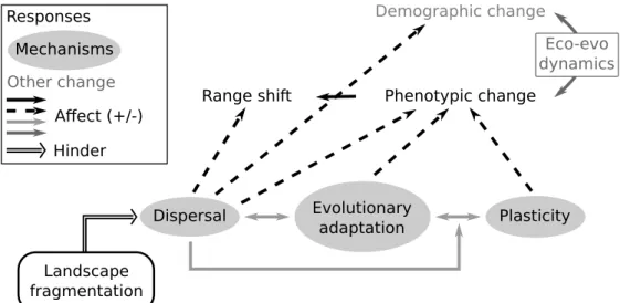
Range shift Demographic change Phenotypic change Dispersal Evolutionary adaptation Plasticity Landscape fragmentation Eco-evo dynamics Responses Mechanisms Other change Aﬀect (+/-) Hinder

Figure 1.2 – Global synthesis of the links between the population responses to climate change, their underlying mechanisms and landscape fragmentation

(23)

However, all these predictions rely on the fact that dispersal is considered as ran-dom. Dispersal, though, is increasingly recognized to be a non-random process (Clobert

et al., 2001; Bowler & Benton, 2005; Edelaar et al., 2008; Clobert et al., 2009, 2012;

Ede-laar & Bolnick, 2012; Travis et al., 2012; Lowe & McPeek, 2014). Dispersers are often characterized by a combination of traits promoting movement (i.e. dispersal syndrome, Clobert et al., 2009; Ronce & Clobert, 2012; Cote et al., 2017). The different stages of this process (i.e. departure, transience and settlement) are influenced by individual phenotype, local context and often their match (i.e. matching habitat choice). Variation in the phenotype of individuals may imply variation of fitness in specific environments which should select for inter-individual differences in emigration and immigration deci-sions according to their fit to local environmental conditions (Edelaar et al., 2008). In contrast to random dispersal, where individuals move independently of their fitness ex-pectation, individuals are expected to move from habitats where they expect a low fitness and to settle in habitats where they expect a higher fitness, making dispersal an adap-tive process. Non-random dispersal, and matching habitat choice in particular, has been demonstrated in various species (e.g. insects (Karpestam et al., 2012); fishes (Bolnick

et al., 2009); birds (Dreiss et al., 2012; Camacho et al., 2016; Benkman, 2017); reptiles

(Cote & Clobert, 2007b; Cote et al., 2008)), for different phenotypic traits matching dif-ferent environmental conditions. For example, in three-spine sticklebacks Gasterosteus

aculeatus, a mark–transplant–recapture experiment showed that dispersers’ preferences

for lake and stream habitats depended on lake-like and stream-like morphological at-tributes (Bolnick et al., 2009). Moreover, a recent study demonstrated that dispersal decisions of an ectotherm species depend on the match between individuals’ phenotype and climatic conditions (Bestion et al., 2015a).

Under variable environmental conditions, matching habitat choice and ensuing adap-tive gene flow may locally promote an efficient shift in mean populations’ phenotypes and therefore may influence species’ responses to climate change (Edelaar & Bolnick, 2012). Non-random dispersal and ensuing adaptive gene flow could also modify the expected links between phenotypic plasticity, evolutionary adaptation and dispersal. As

(24)

individu-als should move into habitat where they are adapted, the benefit of phenotypic plasticity should be reduced (Scheiner, 2016) whereas genetic adaptation should be favored. In that case, matching habitat choice can be seen as a plastic response, where individuals are able to adjust their position in space according to their phenotype and the local environ-ment, rather than adjusting their phenotype (i.e. phenotypic plasticity). Furthermore, as climate warming is expected to increase local mismatch between individual phenotypic optimum and local temperature, matching habitat choice may make movements towards more suitable climatic conditions easier and promote an efficient shift of species geographic distribution (Edelaar & Bolnick, 2012).

2.3 Impacts of landscape fragmentation on dispersal and species

responses to climate change

Landscape fragmentation limits dispersal (Figure 1.2) by decreasing the probability for individuals to find a suitable habitat and increasing their mortality during transience (Johannesen et al., 2000; Fahrig, 2003; Bonte et al., 2012). Furthermore, landscape frag-mentation could reduce the adaptiveness of gene flow by hindering the optimality of dispersal decisions. Fragmentation indeed magnifies dispersal costs and should there-fore hamper the exploration of surrounding habitats, reducing the optimality of dispersal decisions (Jacob et al., 2015a; Cote et al., 2017). As a consequence, landscape fragmen-tation could affect the two responses to climate change developed earlier in this section (i.e. range shift and population phenotypic changes). In fragmented landscapes, individ-uals may fail to follow the suitable climatic conditions, limiting the potential for species range shift (Warren et al., 2001; Opdam & Wascher, 2004; Selwood et al., 2015; Fourcade

et al., 2017). During climate change, fragmentation may also prevent individuals to access

microclimatic refuges which could avoid individuals to suffer from extreme climatic con-ditions (Scheffers et al., 2014; Suggitt et al., 2018). As a result, landscape fragmentation may strengthen the climatic impacts on populations. Finally, landscape fragmentation should reduce gene flow among populations, limiting the input of new genotypes which could be selected for and hindering the beneficial effect of adaptive gene flow on genetic

(25)

adaptation.

Landscape fragmentation should thus affect species responses to climate change by modifying the relative influence of the different mechanisms behind these responses. By limiting spatial range shift, landscape fragmentation could raise extinction risk (Warren

et al., 2001; Opdam & Wascher, 2004; Jetz et al., 2007; Brook et al., 2008; Hof et al., 2011;

Comte et al., 2016; Pereira et al., 2010). Population persistence will then rely mainly on population phenotypic change. The relative influence of phenotypic plasticity, evolution-ary adaptation and dispersal on population phenotypic change will also be shaped by landscape structure. By hampering dispersal, landscape fragmentation should enhance selective pressures on phenotypes as individuals could not escape from the stressful en-vironmental conditions. The relative influence of phenotypic plasticity and evolutionary adaption will then depend on the genetic diversity, the capacity for plasticity, the cost associated with this plasticity and whether plasticity is adaptive or maladaptive. Devel-opment of studies tackling how landscape fragmentation modifies the relative influence of the different mechanisms behind species responses to climate change is urgently needed to better predict the future of biodiversity in the face of anthropogenic perturbations.

3 How to study species response to climate change

in fragmented landscape

Complementary approaches can be used to study species response to climate change. Long term study of natural populations is often used to observe the consequence of climate change on populations (e.g. Réale et al., 2003; Charmantier et al., 2008; Massot et al., 2017; Lane et al., 2018). Such studies benefit from large datasets allowing to quantify precisely impacts on populations and to distinguish between plastic and evolutionary re-sponses though the use of quantitative genetic approaches (Kruuk et al., 2014). However, long term datasets are rare and require important time investment and fieldwork survey. Spatial studies regarding the link between climatic conditions and population composi-tion and dynamics could also be used to predict the consequence of climate change in

(26)

a space-for-time substitution (e.g. Skelly & Freidenburg, 2000; Kealoha Freidenburg & Skelly, 2004). For example studies of different populations distributed on a latitudinal or altitudinal gradient could help understand how population compositions are shaped by the local climatic conditions and could be extrapolated to a context of climate change. However, space-for-time substitution induces other biases; studies along altitudinal gra-dient may, for instance, fail to distinguish between pressures induced by temperature and oxygen concentration. In a context of global change, using studies of natural popula-tions to assess species responses to multiple drivers (e.g. climate change and landscape fragmentation) could be hard to accomplish. For instance, to study population responses to climate change and landscape fragmentation, it would require the survey of different populations inhabiting landscapes more or less fragmented to be able to distinguish the effect of each driver and their interaction. Studies of natural population indeed often fail to distinguish between the effects of different drivers of global change on populations. These studies could also suffer from the limited number of replicated sites. Experimental approaches could be an easier way to study combined drivers of global change.

Experimental approaches allow to test for the combined influence of climate change and other drivers of global change on biological systems, by manipulating these drivers in a crossed design. Experiments manipulating climatic variables have already been devel-oped in many taxa (e.g. Benedetti-Cecchi et al., 2006; Wernberg et al., 2012; Wolkovich

et al., 2012; Bestion et al., 2015a,b; Davenport et al., 2017). Moreover, experiments could

help distinguish between plastic and evolutionary responses to climate change (i.e. exper-imental evolution, transplant experiment, common garden experiment (Merilä & Hendry, 2014)). For instance, experimental evolution allows to directly link the observed pheno-typic change to the conditions which have been manipulated rather than using correlative approaches. Moreover, it often allows to manipulate multiple drivers of global change si-multaneously (e.g. Davenport et al., 2017). Different methods can be used to distinguish between evolutionary adaptation and phenotypic plasticity in experimental evolution. The use of quantitative genetic approaches can be used if the pedigree of the individuals is known. Common garden experiment can also determine if the experimental treatments

(27)

led to evolutionary adaptation. Common garden experiment consists in raising individ-uals from different populations/conditions into standardized and common laboratory or field conditions (Merilä & Hendry, 2014). If the difference among populations/conditions remain after at least one or two generations of common garden (to minimize interference from maternal effects and acclimation (Stoks et al., 2014)), we can conclude that evolu-tionary adaptation played a role in population differentiation. However, experiments are often limited in space and time. It could be thus difficult to make clear predictions on the long-term effect of global change on biodiversity with experiments only. The development of theoretical models, integrating parameters extracted from experiments, could then be needed.

Theoretical models could either be used to predict future distribution of particular species (e.g. bioclimatic envelop models (Thuiller et al., 2005)) or to test for the influ-ence of specific mechanisms in species response to climate change (e.g. biotic interactions (Bocedi et al., 2013); pollen dispersal (Aguilée et al., 2016)). Models allow to make predic-tions on large spatio-temporal scales, according to different climatic scenarios, landscape structures and species characteristics (e.g. Thomas et al., 2001). Models could also be used to develop theoretical predictions, which could be validated (or invalidated) with the use of data on natural populations. The coupling of approaches is thus often needed to make reliable predictions and override the limits of each approach.

Especially, the coupling of models and experiments could be used in two different ways; experiments could be performed following model development to validate theoretical pre-dictions (e.g. Fronhofer et al., 2017); experiment could also precede model development. Experiment could indeed bring light on biological mechanisms which could be then in-tegrated into a model to test their influence on larger spatio-temporal scales (e.g. Jacob

et al., 2018). Under climate change, significant improvements are needed to better

pre-dict future species distribution (Urban et al., 2016). Experiments could help increase our knowledge on the interacting effect of climate change and habitat fragmentation on species persistence. For instance, the relative influence of dispersal, phenotypic plasticity and evo-lutionary adaptation in population response to climate change could be experimentally

(28)

tested. Mechanisms of dispersal and its influence on population adaptation, range shift and species persistence, depending on landscape configuration, could then be explored theoretically to provide more reliable predictions and set up efficient management policies and conservation plans.

4 Objectives

My PhD project aimed at improving our understanding on species responses to the combined effect of climate change and landscape fragmentation. I was especially interested in how dispersal, shaped by landscape structure, could affect species responses to climate change and modulate population adaptation to new climatic conditions. In 2015, Elvire Bestion defended her PhD thesis entitled “Impacts of climate change on a vertebrate ectotherm: from individuals to the community”. During her PhD, she performed exper-iments on the common lizard and demonstrated that during one-year long experiment,

a 2◦C warmer condition accelerate the pace of life of individuals and may affect

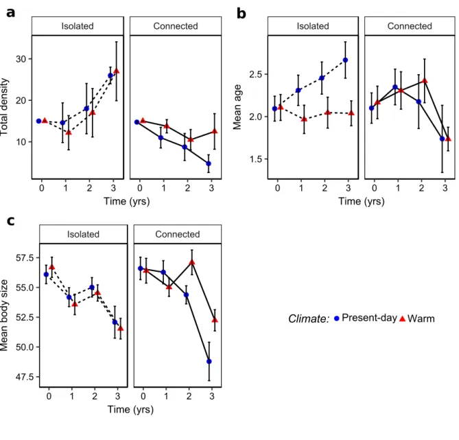
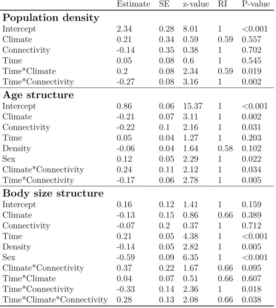
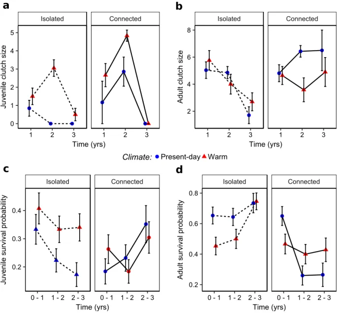
popula-tion persistence when these populapopula-tions were isolated (Bespopula-tion et al., 2015b). However, a longer period of time is required to assess the effect of accelerated pace-of-life syndrome on population dynamics. The accelerated pace-of-life syndrome, if maintained on a longer period of time, should lead to changes in the age and size structure of populations. How-ever, evolutionary and plastic processes could enhance or buffer the accelerating effect of warmer temperature on individual pace of life and change the predictions about popula-tion dynamics. I therefore tested, as a first empirical objective, how climatic condipopula-tions influence population dynamics (Chapter 2) and population adaptation (Chapter 3) using a 3-years long experiment.

My second objective was to study how the connectivity among habitats could modulate the impacts of climatic conditions on population dynamics and adaptation. Landscape connectivity may change the effect of climate change in different ways. First, landscape connectivity allows the movements between microclimates, which may constitute micro-climate refuges and slow down the impacts of micro-climate change on population dynamics. Second, it allows a gene flow between habitats which adds up to the two other

(29)

mech-anisms underlying population adaptation, phenotypic plasticity and evolutionary adap-tation. The relative influence of these 3 mechanisms in population response to climate change is still poorly studied. Moreover, common lizard has been demonstrated to per-form matching habitat choice (Bestion et al., 2015a). Matching habitat choice should thus promote population adaptation to local climate in connected landscapes (Edelaar & Bolnick, 2012; Bolnick & Otto, 2013; Scheiner, 2016; Edelaar et al., 2017). Landscape frag-mentation should alter the relative influence of evolutionary adaptation and phenotypic plasticity on population response to climate change by preventing dispersal. I used an experimental approach to study how evolutionary adaptation, dispersal and phenotypic plasticity shape population phenotypic response to different climatic conditions. To do so, I manipulated the connectivity between habitats to understand how connectivity between microclimates could modify the effect of climate on population dynamics (Chapter 2) and to quantify the role of the different mechanisms involved in population phenotypic change (Chapter 3).

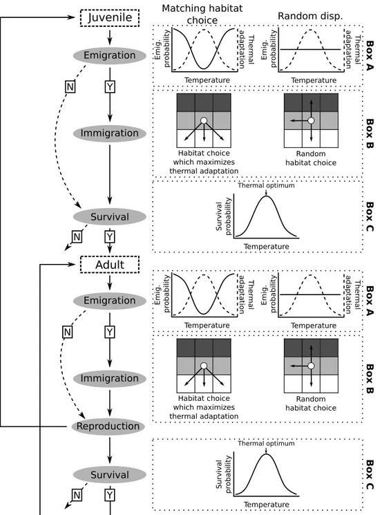
My third objective was to understand how matching habitat choice could modify species response to climate change on large spatio-temporal scales. Matching habitat choice linked to climatic conditions, as demonstrated in Bestion et al. (2015a), could strongly affect species response to climate change. Under stable environment, previous models predicted that matching habitat choice should promote adaptive gene flow (Holt, 1987; Jaenike & Holt, 1991; Ruxton & Rohani, 1999; Armsworth & Roughgarden, 2005b, 2008; Bolnick & Otto, 2013; Scheiner, 2016) and favor population adaptation and dif-ferentiation on small spatiotemporal scales (Edelaar & Bolnick, 2012; Bolnick & Otto, 2013; Scheiner, 2016; Edelaar et al., 2017). Under climate change, matching habitat choice could also promote an efficient shift of species geographic distribution (Edelaar & Bolnick, 2012), increasing species persistence. However, this verbal prediction has never been tested. I used a modeling approach to test how matching habitat choice modifies predictions of future species distribution under climate change (Chapter 4).

(30)

5 General methods

To reach these objectives, I used a combination of approaches allowing both to under-stand how populations respond to climate change in fragmented or continuous landscape and to test for the influence of matching habitat choice on species persistence under climate change. I used experimental and modeling approaches to tackle these questions.

5.1 The experimental approach

I used experiments to study population responses to climate change in fragmented and continuous landscape (chapter 2 and 3). The use of experiments allows to manipulate the drivers of interest rather than using correlative approaches. Moreover, it helps to distinguish between the processes behind population responses to climate change. Merilä & Hendry (2014) reviewed the methods which could be used to distinguish evolutionary adaptation from phenotypic plasticity. Among these methods, the use of experimental approaches such as experimental evolution and common garden experiments are of central interest to better understand how selective pressures and plasticity shape phenotypic responses to climate change. Moreover, landscape structure can be “easily” manipulated to test for the influence of dispersal on population response.

I performed a 3-years long experiment using populations of the common lizard (Zootoca

vivipara) subjected to different climatic conditions and connectivity treatments. During

three years, populations were inhabiting enclosures of an experimental system, the Meta-tron, allowing to manipulate climatic conditions and connectivity among populations. We monitored population composition and dynamics through time and measured evolu-tionary and plastic processes as well as dispersal. After the three years of treatments, the individuals were redistributed among the climatic conditions to test whether changes regarding the treatments induced advantages in the different climatic conditions.

(31)

The common lizard

The common lizard (Zootoca vivipara, Figure 1.3) is a small viviparous lacertid (adult snout-vent length = 50-70 mm). Its dorsal coloration is highly variable, ranging from light to dark brown, with some green reflects, and its ventral coloration ranges from pale yel-low to dark orange. It spreads across Eurasia, from Ireland to Japan and northern Spain to Scandinavia (Figure 1.4), and can be found from sea level to high altitude (2900m (Agasyan et al., 2010)). It inhabits a great variety of habitats including grassland, mead-ows, humid scrubland, hedgermead-ows, open woodland, woodland edges, peat bogs, stream edges, coastal areas and rural gardens (Agasyan et al., 2010) and feeds on a great variety of prey including spiders, Coleoptera, Orthoptera, Heteroptera, Homoptera, Diptera, Hy-menoptera, Gasteropods, Isopods and Lepidoptera caterpillars, with Aranae, Orthoptera, Heteroptera and Homoptera being its favorite preys (Avery, 1966; Pilorge, 1982; González-Suárez et al., 2011). The average lifespan of this species is five years (Sorci & Clobert, 1999) but females can reach up to 11 year-old and males up to 7 year-old (Richard

et al., 2005). Three age stages can be distinguished: juvenile (<1 year-old), yearlings

(1 to 2 year-old) and adults (>2 year-old). Most natural populations are composed of ovoviviparous individuals, except some populations in the southern portion of the range which are oviparous (Surget-Groba et al., 2006). Reproduction is mainly made by > 2 year-old individuals (Massot et al., 1992), even if yearlings can also reproduce depending on their body size (Richard et al., 2005; Bestion et al., 2015b).

Common lizards hibernate from November to February in our study system (Ariège, France). Males emerge from hibernation one or two weeks before yearlings and females and mating starts right after females’ emergence. Female reproduce with up to 7 males and males reproduce with up to 12 females (Richard et al., 2005; Eizaguirre et al., 2007). Gestation time depends on external temperature, but lasts generally two to three months. Females lay around 5 (1-12) soft-shelled eggs (Massot et al., 1992). Parturition starts in June and all parturition occurred in a period of one month on average. Juveniles emerge from the eggs within one hour after parturition and are directly independent (Massot

(32)

Figure 1.3 – Lizards thermoregulating into an enclosure of the Metatron. a,e,f) Juvenile individuals, b) adult male individuals and c,d) adult female individuals. The female in picture d) finishes moulting

Figure 1.4 – Distribution area of the common lizard Zootoca vivipara. Source: IUCN spatial distribution data

± 0.03g in our experiment. There is a high mortality during the juvenile stage as 75% of juveniles die the first year.

Individuals disperse mostly at the juvenile stage (Le Galliard & Clobert, 2003), but yearlings and adults also disperse to a lower extent. Adult home range of common lizard is around 20 meters (Clobert et al., 1994), and dispersal distance varies between 19 and 100 m (Clobert et al., 1994, 2012). In this species, dispersal has been shown to be influenced by extrinsic factors (e.g. density (Clobert et al., 1994; Le Galliard & Clobert, 2003; Cote & Clobert, 2007b), temperature (Massot et al., 2008), kin competition (Cote & Clobert, 2007b, 2010)), intrinsic factors (e.g. body size (Clobert et al., 1994; Cote & Clobert, 2010), maternal effects (Clobert et al., 1994; Cote & Clobert, 2010, 2007b), social traits

(33)

(Cote & Clobert, 2007b), stress level (Meylan et al., 2002, 2004)) and their interaction (e.g. social behavior and local density (Cote & Clobert, 2007b)).

The common lizard, as all ectotherms, is dependent on external temperature for its physiological functions (Box 1). Physiological traits as well as morphological and be-havioral traits associated with thermoregulation are therefore expected to be affected by contemporary climate change. For instance, the different parameters of thermal perfor-mance curve (Box 1) are crucial parameters for species persistence under climate change. However, their measurements can be challenging, in particular in studies examining the evolutionary and plastic processes behind phenotypic changes, as phenotype has to be measured at the individual level. Proxies for evaluating thermal performance are thus often used to characterize thermal physiology of ectotherms. In lizards, maximal critical thermal limit (CT max), mean body temperature of active lizards in the field and pre-ferred temperature in a laboratory thermal gradient are good proxies of thermal optimum (Huey et al., 2012). Particular phenotypic and behavioral traits could also play a major role in buffering the influence of climate change on ectotherms’ body temperature. For instance, Sinervo et al. (2010) predicted that the increase in external temperature should reduce the period of activity of lizards, leading to 39% of population extinction within species ranges. Behavioral adjustment may allow individuals to change their period of activity to avoid the warmest hours of the day and keep enough activity period for for-aging and others important physiological functions. Individuals could adjust their period of activity by advancing their phenology or adjusting their period of activity within a day. Some morphological characteristics are also known to have a direct effect on body temperature of ectotherms. For instance, the darkness of the individuals affects their body temperature as darker individuals should be more at risk of overheating than paler ones (thermal melanism hypothesis (Trullas et al., 2007)). Focusing on these traits could thus help predict ectotherm responses to contemporary climate change.

Effect of climate change on common lizard populations have been studied using long term monitoring of natural populations (Chamaillé-Jammes et al., 2006; Massot et al., 2008; Lepetz et al., 2009; Le Galliard et al., 2010; Rutschmann et al., 2016; Massot et al.,

(34)

2017) and experimental manipulation (Bestion et al., 2015a,b, 2017). In natural popula-tions of the Cévennes mountains, warmer temperature affected population dynamics by promoting body growth, adult body size and clutch size (Chamaillé-Jammes et al., 2006; Le Galliard et al., 2010), advancing laying date (Le Galliard et al., 2010; Massot et al., 2017), reducing dispersal of juveniles (Massot et al., 2008) and disturbing reproductive tradeoffs (Rutschmann et al., 2016). Warmer temperature also affected phenotypic traits into populations; dorsal pattern distribution changed in response to climate warming (Lepetz et al., 2009). Furthermore, one year experimental manipulations of climatic con-ditions highlighted the effect of warmer climate on life-history traits; warmer temperature accelerated individual pace of life (Bestion et al., 2015b) and affected dispersal patterns through its influence on matching habitat choice (Bestion et al., 2015a). Finally, warmer climatic conditions decreased the diversity of the gut microbiota of lizards (Bestion et al., 2017). All these studies highlight the multiple facets of common lizards’ responses to climate change. More efforts have to be done to better understand how future climatic conditions will shape population dynamics and composition of this species, and of all ectotherms in general, in the context of current global change. I aimed at doing so by using an experimental approach with populations maintained for several generations and manipulating simultaneously climatic conditions and connectivity among habitats.

(35)

Box 1: Thermal physiology of ectotherms in the face of climate change Perfor manc e Body temperature Thermal optimum CTmax CTmin Thermal tolerance

Ectotherm body temperature is directly linked to external temperature and shapes all the behavioral and physiological traits (Angilletta et al., 2002), such as metabolism (e.g. Gillooly et al., 2001; Brown et al., 2004; Dillon et al., 2010), loco-motion (e.g. Bennett, 1990), digestion (e.g. Van Damme et al., 1991) and growth (e.g. Kingsolver & Woods, 1997). The relation between ectotherm physiology and temperature can be described by thermal performance curves (Huey & Steven-son, 1979, see Figure above). These curves are defined by a thermal optimum (i.e. temperature maximizing performance), critical thermal limits (i.e. CT min and

CT max the lower and upper temperature allowing performance respectively) and

a thermal tolerance (i.e. range of temperature allowing performance). Thermal performance curves determine the range of temperature at which a population or an individual can persist. For instance, Sinervo et al. (2010) predicted that climate change could lead to 39% of population extinction. They argue that, in absence of adaptation, body temperature should exceed upper thermal limit, leading to in-dividual death, population extirpation and species extinction. However, thermal performance curves may evolve in response to the increase in temperature (Huey & Kingsolver, 1993; Angilletta et al., 2002). Parameters of thermal performance curves vary among species, populations and individuals (Kealoha Freidenburg & Skelly, 2004; Sunday et al., 2011; Artacho et al., 2013). Natural selection could thus lead to evolutionary adaptation. The link between external temperature and body temperature could also be buffered by phenotypic, physiological and

behav-ioral traits (Angilletta et al., 2002). For example, behavioral thermoregulation

allows individuals to cool themselves by hiding in shade areas, burrows and cooler microhabitats. Thermoregulation permits individuals to live into conditions where external temperature exceeds their thermal limits (Sunday et al., 2014). Such traits could also change plastically or genetically in response to climate change. Moreover, multiple physiological and thermoregulatory traits often covary to form thermal types along a cold-hot continuum (Goulet et al., 2017) that could also evolve to maintain optimal body temperature.

(36)

The Metatron

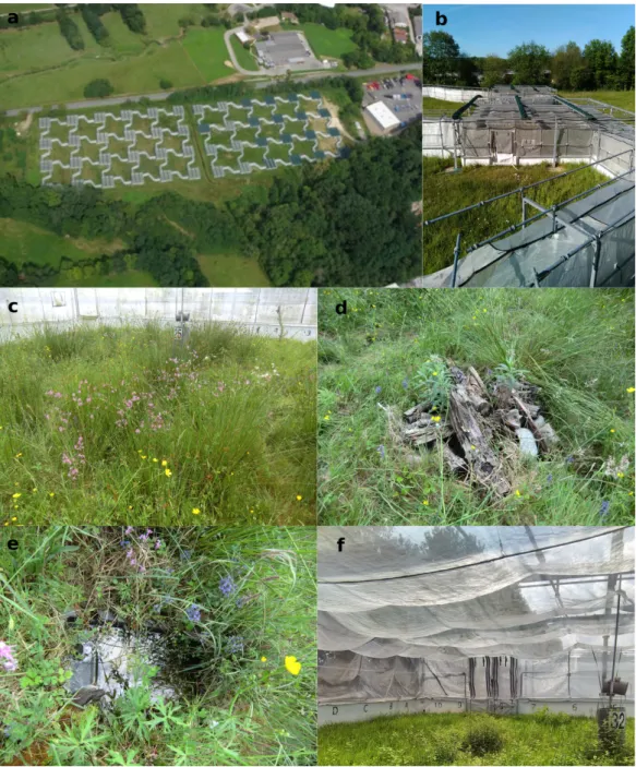
The Metatron (Figure 1.5) is an experimental system situated in the south of France

(Ariège) composed of 48 interconnected semi-natural enclosures of 100 m2 _{surface each}

(Legrand et al., 2012). The enclosure size is equivalent to the common lizards’ core home range size (Clobert et al., 1994; Lecomte & Clobert, 1996; Boudjemadi et al., 1999). Tarpaulins buried in the soil and nets prevent terrestrial and avian predation and lizard escapes. Each enclosure acts as a mini-ecosystem with vegetation, insect communities and habitat heterogeneity with rocks, wood logs for thermoregulation and small water ponds. Enclosures shelter 133 plant species (estimated in June 2018) and at least 82 invertebrate families (mostly arachnids and insects, estimated in 2017).

Enclosures can be connected through a 19 meters corridor, corresponding to the min-imal dispersal distance of the common lizard (Clobert et al., 1994, 2012). Corridors can be easily opened and closed to manipulate landscape connectivity. When corridors are open, lizards could disperse from one enclosure to another.

Temperature, hygrometry and illuminance are automatically recorded every 30 min-utes in each enclosure and can be manipulated via the actuation of motorized shutters and a sprinkler system. For this experiment, we set up two climatic treatments, by closing the shutters at different temperatures. For the “present-day climate” treatment, the shutters

automatically closed when ambient temperature in the enclosures reached 28◦C. For the

“warm climate” treatment, the shutters closed when ambient temperature reached 38◦C.

Given that enclosures are intrinsically warmer than outside, the present-day climate treat-ment allows to obtained thermal conditions similar to the mean temperature outside of the Metatron (temperature in the nearby meteorological station of Saint-Girons Antichan (Bestion et al., 2015a,b)). During the three years of our experiment, the mean summer daily temperatures in the warm climate treatment were on average 1.5 degrees warmer than the present-day climate treatment. Over the three years of experiments, the mean

summer temperature of the present-day climate treatment was 26.03±0.15◦C and the one

for the warm climate treatment was 27.42±0.18◦C. As our treatments depend on outdoor

(37)

-Figure 1.5 – The metatron. a) is a aerial view of the system. b) is a view of an enclosure from outside. c,d,e,f) are views from inside of an enclosure, showing vegetation (c,f), wood logs (d) and water pond (e). We can see the entrance (closed) of a corridor in the background of picture (f)

June to mid - September) and the difference between treatments varied with the weather. The mean summer temperature could therefore be slightly different between the years (26.23±0.25 and 27.71±0.26 in 2015, 26.34±0.24 and 27.88±0.24 in 2016, 25.52±0.24 and 26.67±0.25 in 2017 for present-day climate treatment and warm climate treatment respectively). Relative to the 1986-2005 period, global mean surface temperature increase

(38)

all scenarii in 2080-2100 except RCP2.6 (IPCC (2014), Table 1.1).

Experimental design and chronology of the experiment (Figures 1.6,1.7)

Present-day climate Warm climate

x4 x4 3 years of e xperiment 3 month s of common ga rden x6

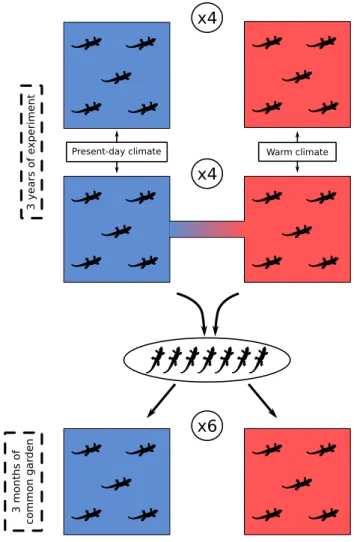
Figure 1.6 – Experimental design of the experiment performed in the Metatron. Pairs of isolated (4 pairs) and connected (4 pairs) enclosures (with one present-day (blue) and one warm (red) climate) were built. Populations of lizards were introduced and lived there for 3 years. We then performed a reciprocal common garden experiment into 12 enclosures, 6 with present-day climate (blue) and 6 with warm climate (red). The individuals were split between the two treatments of the common garden (see details in Chapter 3). The reciprocal common garden lasted three months

Our experimental design consisted in 16 enclosures with two climatic and two con-nectivity treatments (Figure 1.6). Populations of lizards were maintained in the system for three years. At the end of these three years of treatments, we did a reciprocal com-mon garden experiment to test whether the changes in phenotypes resulted in differences in individuals’ success in the different climatic conditions. Compared to a classic com-mon garden, where all the individuals are raised in the same condition, we distributed

(39)

the individuals in the two climatic conditions. We used 12 isolated enclosures, 6 with a present-day climate treatment and 6 with a future warm climate treatment. The re-ciprocal common garden lasted 2.5 months, from July to mid September 2018. Because of the short period of time, and because we did not measure phenotypes at the end of the reciprocal common garden, we did not use it to distinguish between evolutionary and plastic processes that could occur during the three years of experiment. The chronology of the experiment is described in Figure 1.7. More details about experimental design and chronology are provided in Chapters 2 and 3.