Comparison of 2D turbulence models for steady flows computation in a macro-rough channel

Comparison of 2D turbulence models for steady flows computation in a

macro-rough channel

S. Erpicum

HACH – ArGEnCo - University of Liege, Liege, Belgium

T. Meile

LCH – Ecole Polytechnique Fédérale de Lausanne (EPFL), Lausanne, Switzerland

B.J. Dewals

HACH – ArGEnCo - University of Liege, Liege, Belgium

Belgian National Fund for Scientific Research (FRS-FNRS), Brussels, Belgium

A. Schleiss

LCH – Ecole Polytechnique Fédérale de Lausanne (EPFL), Lausanne, Switzerland

M. Pirotton

HACH – ArGEnCo - University of Liege, Liege, Belgium

ABSTRACT: A 2D numerical flow model, developed at the Laboratory of Hydrology, Applied Hydrodynam-ics and Hydraulic Constructions (HACH) at ULg, has been applied to flows in a macro-rough channel using three different approaches to compute the turbulence effects. Both the first and second ones are based on al-gebraic expressions of the turbulent viscosity, and the third one uses a depth-integrated k-ε type model involv-ing two additional partial differential equations. Data for the comparison have been provided by experiments conducted at the Laboratory of Hydraulic Constructions (LCH) at EPFL, showing different two-dimensional flow characteristics in varied configurations of large scale cavities in depressions at the side walls of the flume. Despite the strongly different modeling approaches used in the three models to handle the turbulence effects, the numerical models give generally similar and satisfactory agreement between experimental and numerical results regarding backwater curves.

1. INTRODUCTION

A depth integrated approach for flow modeling, tak-ing into account a hydrostatic pressure distribution, is generally suitable for many problems encountered in rivers, especially when modeling flows in chan-nels with rather flat bottom.

Although turbulence effects are neglected in many practical engineering applications, especially if ex-ternal forces due to the solid boundary friction are predominant (steady flow) or if major advection ef-fects are present (unsteady flow), the predominance of transport terms in the hydrodynamic equations can be less important, mainly in low velocity flows, close to hydraulic structures or for specific geome-trical configurations which lead to an increasing ef-fect of recirculation currents and velocity gradients.

Various approaches exist to handle turbulence ef-fect in the shallow water equations, as rather simple algebraic expressions of turbulent viscosity (i.e. Fisher et al. 1979, Hervouet 2003) or more complex models involving additional equations (i.e. Rastogi & Rodi 1978, Rodi 1984, Babarutsi & Chu 1998).

In this paper, three different turbulence models, integrated into the shallow water equations, are ap-plied to backwater-curve computations in a laborato-ry channel with large scale cavity roughness at both banks. The geometrical configurations of macro-roughness investigated with systematic hydraulic model tests produce recirculation zones, vertical mixing layers and wakes due to high velocity gra-dients in the main flow plane (Meile 2007).

In the first turbulence modeling approach, the turbulent viscosity is computed proportionally to the friction velocity (Fisher et al. 1979). In the second one, it is evaluated on the basis of the mean velocity gradients in the main flow plane (Hervouet 2003). The third model (Erpicum 2006) differentiates the large-scale transverse-shear-generated turbulence, associated with the horizontal length-scale of the flow, and the small-scale bed-generated one, with a characteristic dimension equal of the water depth, as suggested by Babarutsi & Chu (1998).

As shown by Erpicum (2006), the third model has already proven its relevance on test cases from the literature such as for flows through a sudden

en-25 x [m] 20 15 10 5 0 30 35 Prismatic 221 121 224 124

Inlet reach Reach with macro-scale roughness Outlet reach Lb Lc

ΔB B

Table 1. Geometrical characteristics and specific discharges [m²/s] of the selected channel configurations

Figure 1. Plane views of the flume in the selected channel

con-figurations. Position of the ultrasonic elevation probes (z).

largement (Babarutsi et al. 1989) and in a channel

with a groin (Rajaratnam & Nwachukwu 1983). Its application to backwater-curve computations is de-picted in details in Erpicum et al. (submitted).

2. PHYSICAL EXPERIMENTS

Hydraulic model tests have been performed by Meile (2007) in a flume with a useful length of 38.33 m and a mean bed slope of 1.14 ‰. From up-stream to downup-stream, the channel is divided into an inlet reach, a reach with large scale cavity roughness at the banks and an outlet reach (Fig. 1). The chan-nel bottom is made of painted steel and the sidewalls of the reach, including the large scale rectangular cavities in depressions, are formed by smooth limes-tone bricks. The channel bed is fixed and no sedi-ment transport has been taken into account.

The constant channel base width is

B = 0.485 ± 0.002 m. Three geometrical parameters,

namely the length of the cavity Lb, the distance be-tween two cavities Lc and the depth of the cavities

ΔB (Fig. 1), have been systematically varied. The

combination of three different values for Lb and Lc and four different values of ΔB results in 36

differ-ent, axi-symmetric geometrical configurations cov-ering 8 aspect ratios AR = ΔB / Lb and 4 expansion ratios ER = (B + 2ΔB) / B. Additionally, a prismatic

and a randomly generated configuration have been analyzed. (Meile 2007)

The discharge, introduced at the upstream border of the channel through a horizontal opening of the inlet basin, was controlled by an electromagnetic flow meter. At the downstream border of the chan-nel, the flow depth was controlled by a particularly shaped cross section. It corresponded almost to the normal flow depth of the prismatic channel without macro-roughness. During the tests, the water levels have been recorded with ultrasonic elevation probes located along the channel axis. The accuracy of the measurements is at least ± 0.002 m. The ultrasonic elevation probes have been placed in the small channel sections or at the beginning, in the middle and at the end of the widened channel reaches (Fig. 1). Thus, variations of the flow depth at specif-ic locations can be evaluated.

Characteristic values of Froude Fr = U(gh)-1/2 and Reynolds Re = URhν -1 numbers relative to the base width B ranged between 0.37 < Fr < 0.64 and

6’800 < Re < 110’000 for typical flow depths be-tween 0.03 m < h < 0.34 m and mean flow velocities between 0.24 ms-1 < U < 0.80 ms-1. U is the mean flow velocity in the cross-section and Rh is the hy-draulic radius, both calculated relative to the small channel section at base width B.

Four out of the 36 different geometrical configura-tions (Fig. 1 & Table 1) have been selected to be in-vestigated with a 2D numerical model using a two length scale, depth integrated k-ε type approach for turbulence modeling (Erpicum et al. submitted). Fur-thermore, the prismatic channel served as a refer-ence for the calibration of the bottom and wall sur-face roughness. In this paper, we focused on these four specific configurations for three discharges cor-responding to the minimum, maximum and medium amplitudes considered by Meile (2007) (Table 1).

The choice of the test cases has been motivated by the different cavity flow types identified in the experimental study, namely the square grooved flow type (124), the reattachment flow type (221) and the normal recirculating flow type (121 & 224).

3. NUMERICAL MODEL

The flow model is based on the two-dimensional depth-averaged equations of volume and momentum conservation (Shallow Water Equations)

0 h hu hv t x y ∂ ∂ ∂ + + = ∂ ∂ ∂ (1) 2 2 2 0 b x yx xx z hu hu huv g h gh ghJ t x y x x h h x y τ τ ∂ ∂ ∂ ∂ ∂ + + + + − ∂ ∂ ∂ ∂ ∂ ∂ ∂ + + = ∂ ∂ (2) Config. Lb [m] Lc [m] Δ B AR [-] ER [-] q1 q2 q3 Prismatic - - - .0134 .0996 .2781 221 1.0 1.0 0.1 0.1 1.41 .0100 .1006 .2149 121 0.5 1.0 0.1 0.2 1.41 .0114 .1033 .2189 224 1.0 1.0 0.4 0.4 2.65 .0108 .0999 .2186 124 0.5 1.0 0.4 0.8 2.65 .0130 .0971 .1311

2 2 2 0 b y xy yy z hv huv hv g h gh ghJ t x y y y h h x y τ τ ∂ ∂ ₊∂ ₊∂ ₊ ∂ _{+ −} ∂ ∂ ∂ ∂ ∂ ∂ ∂ + + = ∂ ∂ (3)

where is the water depth, u _{and are the}

depth-averaged velocity components, is the bottom ele-vation,

h v

b z x

J and _{J are the friction slope components, y} xx

τ and τ_{yy are the viscous and turbulent normal} stresses and τ_xyand τ_{yx are the viscous and turbulent} shear stresses.

The bottom friction is conventionally modeled with an empirical law, such as the Manning formula. In addition, the friction along side walls is reduced through a process-oriented formulation pro-posed by Dewals (2006). Finally friction terms write

2 2 2 2 b 4/ 3 1/3 1 4 3 x x N x k n n J u u v u h = h ⎡ ⎢ ⎢⎣ = + + Δ

∑

w y ⎤ ⎥ ⎥⎦ (4) 2 3/ 2 2 2 b 4 / 3 1/ 3 1 4 3 y y N y k n n J v u v v h = h ⎡ ⎢ ⎢⎣ = + + Δ

∑

w x ⎤ ⎥ ⎥⎦ (5)

where the Manning coefficients nb and nw character-ize respectively the bottom and the side-walls roughness. These relations have been written for Cartesian grids used in the present study.

Three different models have been used to compute the turbulent stresses terms in Eq. (2) and (3). Both the first and second ones use the Boussinesq as-sumption (Boussinesq 1877) transposed to depth in-tegrated variables (Erpicum 2006) to model the tur-bulent stresses xx yy t u v x y τ = −τ =ν ⎛_⎜∂ −∂ ⎞_⎟ ∂ ∂ ⎝ ⎠ (6) xy yx t v u x y τ =τ =ν ⎛_⎜∂ +∂ ⎞_⎟ ∂ ∂ ⎝ ⎠ (7)

where ν_{t is the turbulent viscosity. This new} varia-ble is evaluated by means of a analytical expression of the local mean flow variables. Both models are thus based on a local equilibrium assumption be-tween turbulence production and dissipation.

In the first approach (model 1), the turbulent vis-cosity is computed proportionally to the friction ve-locity, as proposed by Fisher et al. (1979) for river flows where the turbulence is mainly governed by bottom friction

*

t hU

ν =α (8)

where U* _{is the friction velocity and}

α

_{a coefficient}

equal to 0.5 as suggested by Fisher et al. (1979).

The second approach (model 2) is based on the mixing length assumption to compute the turbulent viscosity with an expression suggested by Smago-rinski (Hervouet 2003) 2 2 2 2 2 t u v u x y v x y y x ν = Δ Δα _⎜⎛∂ ⎞_⎟ + _⎜⎛∂ ⎞_⎟ +⎛_⎜∂ +∂ ⎞_⎟ ∂ ∂ ∂ ∂ ⎝ ⎠ ⎝ ⎠ ⎝ ⎠ (9)

where the proportionality coefficient α _{has been} chosen equal to 1. In this model, following the Prandtl assumption, the mixing length is the space discretization step and the mean fluctuation velocity is related to the depth averaged velocity gradients. Thus, this model considers the turbulence effects generated in the main flow plane at a scale smaller than the mesh size (sub-grid model).

The third model (model 3) is a depth-integrated

k-ε type model involving two additional partial diffe-rential equations (Erpicum 2006). As suggested by Babarutsi & Chu (1998), it differentiates the large-scale transverse-shear-generated turbulence, asso-ciated with the horizontal length-scale of the flow, and the small-scale bed-generated turbulence, with a characteristic dimension in the order of the water depth.

The model has been built following a two-step Reynolds averaging procedure of the equations of motion, as suggested by Babarutsi & Chu (1998). The first stage filters out the bed-generated turbu-lence by treating the small scale fluctuations of the instantaneous three-dimensional velocity compo-nents with an algebraic model. The second stage considers the transverse-shear-generated turbulence by means of additional fluctuations of the mean ve-locity components in the main flow plane, modeled by two additional transport equations: one for the depth-averaged turbulent kinetic energy k’, and one for the depth-averaged turbulence dissipation rate ε’.

The two step averaging procedure modify the flow motion equations (2) and (3) by adding a k ′gradient term along respectively x- and y-axis. The viscous and turbulent stresses are the sum of three terms representing the viscous effects τ , the bed-V generated turbulence contribution and the large-scale transverse-shear-generated turbulence one . ,3 T τ D ,2 T D τ

In analogy with the general formulation for a Newtonian fluid, the gradients of the depth-averaged viscous stresses terms are modeled, for example along x-direction, as 2 2 V V xy xx h h uh uh x y x τ τ ∂ _ν⎛ ⎞ ∂ _{+ =} ∂ ₊∂ ⎜ ⎟ ∂ ∂ _⎝ ∂ ∂y _⎠ (14)

The corresponding turbulent stresses gradients as-sociated to bed-generated turbulence are modeled in the same manner, following an approach similar to the one of Chapmann & Kuo (1985)

,3 ,3 2 2 ,3 T D T D xy xx T D h h uh uh x y x τ τ ∂ _ν ⎛ ∂ ∂ ∂ + = _⎜ + ∂ ∂ _⎝ ∂ ∂y _⎠ ⎞ ⎟ (15) The corresponding turbulent viscosity ν_T,3D is computed using a local equilibrium assumption with Eq. (8). The α coefficient value is decrease to 0.08 as suggested by Babarutsi (1991).

The turbulent stresses terms associated to large-scale transverse-shear-generated turbulence are modeled by a Boussinesq-type approximation. For example x-momentum equation terms write

,2 ,2 T D xx T D uh vh h k x y τ =ν ⎛_⎜∂ −∂ ⎞_⎟ ′ ∂ ∂ ⎝ ⎠− (16) ,2 ,2 T D xy T D uh vh h y x τ =ν ⎛_⎜∂ +∂ ⎞_⎟ ∂ ∂ ⎝ ⎠ (17)

The associated turbulent viscosity νT,2D is

eva-luated according to Rodi (1984) 2 ,2 T D µ k c ν ε ′ = ′ (18) with c_µ =0.09.

The transport equations for k ′ and ε′ write

* ,2 * ,2 0 T D k T D k k uk vk u v k k t x y x y hk k x h x x x hk k y h y y y P F h ν ν σ ν ν σ ε ′ ′ ′ ∂ ∂ ∂ _′∂ _′∂ + + + + ∂ ∂ ∂ ∂ ∂ ⎛ ⎞ ′ ′ ⎛ ⎞ ∂ ∂ ∂ ∂ + _{⎜ ⎟}+ _{⎜ ⎟} ∂ _⎝ ∂ _⎠ ∂ _⎝ ∂ _⎠ ⎛ ⎞ ′ ′ ⎛ ⎞ ∂ ∂ ∂ ∂ + _{⎜ ⎟}+ _{⎜ ⎟} ∂ _⎝ ∂ _⎠ ∂ _⎝ ∂ _⎠ ′ ′ ′ − + + = (10)

(

)

* ,2 * ,2 2 1 1 3 2 0 T D T D u v t x y h x h x x x h y h y y y c P c F c k ε ε ε ε ε hk ε ε ε ν ν ε ε σ ν ν ε ε σ ε ′ ′ ′ ∂ ∂ ∂ + + ∂ ∂ ∂ ⎛ ⎞ ′ ′ ⎛ ⎞ ∂ ∂ ∂ ∂ + _{⎜ ⎟}+ _{⎜ ⎟} ∂ _⎝ ∂ _⎠ ∂ _⎝ ∂ _⎠ ⎛ ⎞ ′ ′ ⎛ ⎞ ∂ ∂ ∂ ∂ + _{⎜ ⎟}+ _{⎜ ⎟} ∂ _⎝ ∂ _⎠ ∂ _⎝ ∂ _⎠ ′ ′ ′ − ⎡_⎣ − − ⎤_⎦+ ′ ε′ = ′ (11)

where ν* = +ν ν_T,3D is the sum of the water viscosity

ν and of the eddy viscosity ν_T,3D related to bed-generated turbulence. νT,2D is the eddy viscosity

re-lated to the large-scale transverse-shear-generated turbulence.

The production term of turbulence by the trans-verse shear P’ and the term reflecting the effect of bed-friction forces on the turbulence motion F’ are given by equations (12) and (13). The latter has been derived as suggested by Babarutsi & Chu (1998).

,2 T D P uh vh u v x y x y uh vh u v y x y x ν ′ = ⎡⎛_⎢⎜∂ −∂ ⎞⎛_⎟⎜∂ −∂ ⎞_⎟ ∂ ∂ ∂ ∂ ⎝ ⎠⎝ ⎣ ⎤ ⎛∂ ∂ ⎞⎛∂ ∂ ⎞ +_⎜ + _⎟⎜ + _⎟⎥ ∂ ∂ ∂ ∂ ⎝ ⎠⎝ ⎠⎦ ⎠ (12)

(

)

2 ,2 2 2 4 3 _{2 2} 2 2 3 2 T D b F gn k u v h _{u v} uh vh uh vh u v uv x y y x ν ′ = ⎡ ′_⎣ + − + ⎤ ⎛∂ ₋∂ ⎞ _{− +} ⎛∂ ₊∂ ⎞ ⎥ ⎜ _{∂ ∂} ⎟ ⎜ _{∂ ∂} ⎝ ⎠ ⎝ ⎟⎠ ⎦ (13)

The calculations have been performed with a set of coefficients σ_k = , 1.31 σ_ε = , c_1,ε =1.44,

2, 1.92

c _ε = and c_3,ε =0.8 as proposed by Babarutsi & Chu (1998) to model transverse mixing layer in shallow open-channel flows.

System (1), (2) and (3) and possibly (4) and (5) is solved by a finite volume scheme where the fluxes are determined by a Flux Vector Splitting method. The time integration is performed by means of an explicit Runge Kutta algorithm. Specific discharge in the channel is prescribed as inflow boundary con-dition and water surface elevation at the most down-stream probe in the experimental facility is the out-flow one (subcritical out-flow). Regarding boundary condition for the turbulence variables, the shear ve-locity on solid walls is computed according to the law of the wall. The corresponding depth-averaged turbulent variables are calculated, following Rodi (1984) and Younus & Chaudhry (1994), as

( )

2 µ k′ =h Uτ c (19)

( )

3 2 h Uτ d ε′ = κ (20)

where Uτ is the shear velocity assuming a logarith-mic velocity profile near the wall, κ the von Karman constant and d the distance to the wall. Furthermore,

this approach assumes that the laminar boundary layer is within the mesh next to the wall. At inlets, values of 4 2

0 10 0

k′ = − q h and 3 2 0 10 k0

ε′ = ′ h are used (Choi & Garcia 2002), with q0 the specific dis-charge imposed at inlet.

More details on the numerical model can be found in Dewals (2006), Erpicum (2006) or Erpicum et al. (submitted).

4. RESULTS

For calibration of the Manning’s roughness coeffi-cients, the prismatic channel has been modeled using the model 3 and a mesh size of 0.02 m (Erpicum et

al. submitted). The best fit between bottom and si-dewall friction, constant along the channel bottom and the side walls respectively, has been found to be

nb=0.0087 s/m1/3 and nw=0.0105 s/m1/3. The side-walls are rougher than the bottom, in agreement with the experimental facility materials surface patterns. The mean difference between the measured and the computed water depths is lower than the probes ac-curacy (Table 3). From this calibration stage, it has been concluded that without using turbulence terms in a 2D modeling approach, no set of roughness

coefficients can be found to fit the water depth mea-surements in a wide range of discharges.

The application of the models 1 and 2 with the same set of roughness coefficients for both the ex-treme discharges show satisfactory results except for the model 1 with the higher discharge since the dif-ference between the measured and the computed wa-ter depths is twice the probes accuracy (Table 3).

In a second stage, the four configurations with large scale depression roughness at the side walls have been modeled using the three models succes-sively. A mesh size of 0.02 m has been used to

mod-el a length of 36.32 m of the channel. The width

va-ries along the channel, depending on the geometrical configurations. The roughness coefficients values

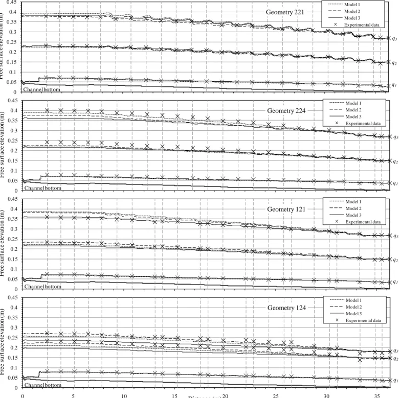
0 0.05 0.1 0.15 0.2 0.25 0.3 0.35 0.4 0.45 0 5 10 15 20 25 30 35 F ree su rf ac e e lev at io n ( m ) Distance (m) Model 1 Geometry 221 Model 2 Model 3 Experimental data q1 q3

Cha nnel bottom

q2 0 0.05 0.1 0.15 0.2 0.25 0.3 0.35 0.4 0.45 0 5 10 15 20 25 30 35 F ree s u rf a ce el e v at io n ( m ) Distance (m) Model 1 Geometry 224 Model 2 Model 3 Experimental data q1 q3

Cha nnel bottom

q2 0 0.05 0.1 0.15 0.2 0.25 0.3 0.35 0.4 0.45 0 5 10 15 20 25 30 35 F ree s u rf a ce el e v at io n ( m ) Distance (m) Model 1 Geometry 121 Model 2 Model 3 Experimental data q1 q3

Cha nnel bottom

q2

Figure 2. Comparison of experimental and simulated backwater curves for the selected macro-rough configurations.

0 0.05 0.1 0.15 0.2 0.25 0.3 0.35 0.4 0.45 0 5 10 15 20 25 30 35 F ree s u rf a ce el e v at io n ( m ) Distance (m) Model 1 Geometry 124 Model 2 Model 3 Experimental data q1 q3

Cha nnel bottom

Config. q1 q2 q3 q1 q2 q3 q1 q2 q3 Prismatic 1.5 - 4.0 1.5 - -2.1 1.4 2.0 1.3 221 -1.1 -3.9 8.2 1.7 -1.0 -2.8 0.5 1.4 4.0 121 -1.9 -4.3 14.6 2.0 3.4 11.0 -0.8 -6.3 0.0 224 -5.9 -13.5 -9.1 -3.6 -9.5 -17.7 -4.8 -12.1 -21.8 124 -2.1 -16.3 -9.2 -1.7 -8.1 -2.9 -2.1 -24.5 -21.7

Absolute value of mean error on water depths [mm] Model 1 Model 2 Model 3

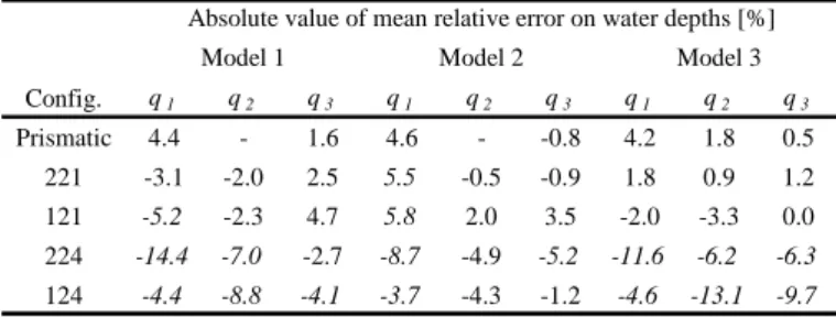
Table 2. Absolute value of mean relative errors between computed and measured flow depths. Errors higher than +/- 5% are indicated in italic

Config. q1 q2 q3 q1 q2 q3 q1 q2 q3 Prismatic 4.4 - 1.6 4.6 - -0.8 4.2 1.8 0.5 221 -3.1 -2.0 2.5 5.5 -0.5 -0.9 1.8 0.9 1.2 121 -5.2 -2.3 4.7 5.8 2.0 3.5 -2.0 -3.3 0.0 224 -14.4 -7.0 -2.7 -8.7 -4.9 -5.2 -11.6 -6.2 -6.3 124 -4.4 -8.8 -4.1 -3.7 -4.3 -1.2 -4.6 -13.1 -9.7

Absolute value of mean relative error on water depths [%] Model 1 Model 2 Model 3

are the ones previously found from the calibration tests. The accuracy of the numerical results has been assessed by a comparison of water depths on 25 points located regularly along the channel axis (Fig. 2, Table 2 and Table 3).

The backwater curves of the configuration with reattachment of the flow to the side walls (221) are well reproduced with the three models. The differ-ence between the measured and computed water depths is in the order of magnitude of the probes ac-curacy (Table 3). The configuration with normal re-circulating flow type and low aspect ratio (121) is also satisfactory reproduced, especially with model 3 (errors less than 5%). The configuration with normal recirculating flow type and high aspect ratio (224) and the one governed by a square grooved flow type (124) show the most important differences between measured and computed flow depths with errors up to 15%. Nevertheless, model 1 succeeds in modeling configuration 124 with errors less than 10% and model 2 shows the same agreement for both confi-gurations 124 and 224.

5. CONCLUSIONS

A 2D numerical flow solver has been applied to flows in a macro-rough channel with three different approaches to model turbulence effects. Data for the comparison were obtained from experiments per-formed with different configurations of large scale cavities at the side walls of a straight channel for a large range of discharges.

Despite the strongly different mathematical ap-proaches, a satisfactory agreement between experi-mental and numerical results could be obtained

re-garding backwater curves with the three turbulence models, especially for the configurations with low aspect ratio.

6. ACKNOWLDGEMENT

The experiments are part of a PhD thesis carried out within the Rhone-Thur national research project “Sustainable use of rivers” granted by the Swiss Federal Office for the Environment (FOEN).

Table 3. Absolute value of mean errors between computed and measured flow depths. Errors higher than the precision of the measurements (± 2mm) are indicated in italic

REFERENCES

Babarutsi, S., Ganoullis, J. & Chu, V.H. 1989. Experimental investigation of shallow recirculating flows. Journal of Hy-draulic Engineering 115(7): 906-924.

Babarutsi, S. 1991. Modelling quasi-two-dimensionnal turbu-lent shear flow. PhD Thesis, Mc Gill University: Montreal Babarutsi, S. & Chu, V. H. 1998. Modeling transverse mixing

layer in shallow open-channel flows. Journal of Hydraulic Engineering 124(7): 718-727.

Boussinesq, J. 1877. Théorie de l’écoulement tourbillonant. Mémoires présentés par divers savants, Académie des Sciences de l’Institut de France 23:45-60.

Chapman, R. & Kuo, C. 1985. Application of the two-equation

k-ε turbulence model to a two-dimensional, steady, free

sur-face flow problem with separation. International Journal for Numerical Methods in Fluids 5: 257-268.

Choi, S.-U. & Garcia, M. 2002. k-ε turbulence modelling of density currents developing two dimensionally on a slope. Journal of Hydraulic Engineering 128(1): 55-63.

Dewals, B.J. 2006. Une approche unifiée pour la modélisation d’écoulements à surface libre, de leur effet érosif sur une structure et de leur interaction avec divers constituants. PhD Thesis, Université de Liège: Liège.

Erpicum, S. 2006. Optimisation objective de parameters en écoulements turbulent à surface libre sur maillage multib-loc. PhD Thesis, Université de Liège: Liège.

Erpicum, S., Meile, T., Dewals, B., Pirotton, M. & Schleiss, A. 2D numerical flow modeling in a macro-rough channel. Submitted to International Journal for Numerical Methods in Fluids.

Fischer, H., List, E., Koh, R., Imberger, J. & Brooks, N. 1979. Mixing in inland and coastal waters. Academic Press: New York.

Hervouet, J-M. 2003. Hydrodynamique des écoulements à sur-face libre - Modélisation numérique avec la méthode des éléments finis. Presses de l'Ecole Nationale des Ponts et Chaussées : Paris

Meile, T. 2007. Influence of macro-roughness of walls on steady and unsteady flow in a channel. PhD thesis No 3952, Ecole Polytechnique Fédérale de Lausanne: Lausanne Rajaratnam, N. & Nwachukwu, B. 1983. Flow near groin-like

structures. Journal of Hydraulic Engineering 109(3): 463-480.

Rastogi, A. & Rodi, W. 1978. Predictions of heat and mass transfer in open channels. Journal of the Hydraulics Divi-sion, ASCE; 104(HY3): 397-420.

Rodi, W. 1984. Turbulence models and their application in hy-draulics - A state-of-the-art (second revised edition). Bal-kema: Leiden

Younus, M. & Chaudhry, M. 1994. A depth-averaged k-ε tur-bulence model for the computation of free-surface flow. Journal of Hydraulic Research 32(3): 415-439.