https://doi.org/10.5194/tc-12-2981-2018
© Author(s) 2018. This work is distributed under the Creative Commons Attribution 4.0 License.
Seasonal mass variations show timing and magnitude of meltwater
storage in the Greenland Ice Sheet
Jiangjun Ran1, Miren Vizcaino1, Pavel Ditmar1, Michiel R. van den Broeke2, Twila Moon3, Christian R. Steger2, Ellyn M. Enderlin4, Bert Wouters2, Brice Noël2, Catharina H. Reijmer2, Roland Klees1, Min Zhong5, Lin Liu6, and Xavier Fettweis7
1Department of Geoscience and Remote Sensing, Delft University of Technology, Delft, the Netherlands 2Institute for Marine and Atmospheric Research, Utrecht University, Utrecht, the Netherlands
3National Snow and Ice Data Center, Cooperative Institute for Research in Environmental Sciences,
University of Colorado, Boulder, CO, USA
4Climate Change Institute and School of Earth and Climate Science, University of Maine, Orono, ME, USA 5State Key Laboratory of Geodesy and Earth’s Dynamics, Institute of Geodesy and Geophysics,
Chinese Academy of Sciences, Wuhan, China
6Earth System Science Programme, Faculty of Science, The Chinese University of Hong Kong, Hong Kong, China 7Department of Geography, University of Liège, Liège, Belgium
Correspondence:Jiangjun Ran (j.ran@tudelft.nl)
Received: 22 February 2018 – Discussion started: 3 April 2018
Revised: 13 August 2018 – Accepted: 22 August 2018 – Published: 21 September 2018
Abstract. The Greenland Ice Sheet (GrIS) is currently los-ing ice mass. In order to accurately predict future sea level rise, the mechanisms driving the observed mass loss must be better understood. Here, we combine data from the satel-lite gravimetry mission Gravity Recovery and Climate Ex-periment (GRACE), surface mass balance (SMB) output of the Regional Atmospheric Climate Model v. 2 (RACMO2), and ice discharge estimates to analyze the mass budget of Greenland at various temporal and spatial scales. We find that the mean rate of mass variations in Greenland ob-served by GRACE was between −277 and −269 Gt yr−1in
2003–2012. This estimate is consistent with the sum (i.e., −304 ± 126 Gt yr−1) of individual contributions – surface mass balance (SMB, 216 ± 122 Gt yr−1) and ice discharge
(520 ± 31 Gt yr−1) – and with previous studies. We further
identify a seasonal mass anomaly throughout the GRACE record that peaks in July at 80–120 Gt and which we interpret to be due to a combination of englacial and subglacial water storage generated by summer surface melting. The robust-ness of this estimate is demonstrated by using both different GRACE-based solutions and different meltwater runoff es-timates (namely, RACMO2.3, SNOWPACK, and MAR3.9). Meltwater storage in the ice sheet occurs primarily due to
storage in the high-accumulation regions of the southeast and northwest parts of Greenland. Analysis of seasonal variations in outlet glacier discharge shows that the contribution of ice discharge to the observed signal is minor (at the level of only a few gigatonnes) and does not explain the seasonal differ-ences between the total mass and SMB signals. With the improved quantification of meltwater storage at the seasonal scale, we highlight its importance for understanding glacio-hydrological processes and their contributions to the ice sheet mass variability.
1 Introduction
During the last decade (2006–2015), the Greenland Ice Sheet (GrIS) has been rapidly losing mass, contributing on average 0.9 mm yr−1 to global mean sea level rise (Enderlin et al.,
2014; Stocker et al., 2013; van den Broeke et al., 2016). The NASA/German Space Agency (DLR) Gravity Recov-ery and Climate Experiment (GRACE) mission is a power-ful tool with which to monitor ice mass variations in Green-land, including the ice sheet and its peripheral glaciers and ice caps, from monthly to multi-year timescales. The total
mass balance (TMB) of the ice sheet represents the summa-tion of processes summarized in Eq. (1): (i) surface mass bal-ance (SMB); (ii) ice discharge (D); and (iii) mass variations (1m/1t), which include all processes not related to SMB and ice discharge, for instance, en- and subglacial meltwater storage. GRACE ice mass balance is calculated after remov-ing the impacts of glacial isostatic adjustment (GIA), atmo-spheric and oceanic variability, and other time-variable geo-physical processes.
TMB = SMB − D + 1m/1t (1)
The quantities in Eq. (1) refer to fluxes (in mass per unit time). Recent GrIS mass loss has been quantified in numer-ous studies (e.g., Shepherd et al., 2012; Schrama et al., 2014; Velicogna et al., 2014). Furthermore, several authors have estimated the contribution to this mass loss from SMB and ice discharge individually (van den Broeke et al., 2009; En-derlin et al., 2014; Velicogna et al., 2014; van den Broeke et al., 2016). To quantify the contribution of SMB, regional climate models (RCMs) are typically used, such as the Re-gional Atmospheric Climate Model v. 2 (RACMO2) (Ettema et al., 2009), Modèle Atmosphérique Régional (MAR) (Fet-tweis et al., 2005, 2017), and HIRHAM (Christensen et al., 1996). The annual ice discharge rates are estimated by com-bining ice flow velocity data and ice thickness data at the flux gates (Thomas et al., 2000). Importantly, ice flow velocities have increased during the last decade and shown different spatial and temporal patterns (Moon et al., 2012).
The analysis of GrIS mass variations at the seasonal timescale is still limited. This is largely because (i) the ac-curacy and spatial resolution of GRACE monthly solutions is relatively poor, as compared to long-term trend estimates, and (ii) ice velocity data at this timescale are scarce (typi-cally, only a few estimates per year are available, often span-ning only a few years). A first attempt to combine GRACE data and SMB modeling in order to evaluate an ice dynam-ics model of the GrIS at the monthly timescale was made by Schlegel et al. (2016). Alexander et al. (2016) examined spa-tial patterns of GrIS seasonal mass variations using a regional climate model, a model of ice dynamics, and GRACE. The seasonal variabilities of the ice velocities of a few marine-terminating glaciers were investigated by, e.g., Howat et al. (2010), Ahlstrøm et al. (2013), and Moon et al. (2015). The only study of multi-regional seasonal variations of GrIS out-let glacier velocities was conducted by Moon et al. (2014), who analyzed 55 marine-terminating glaciers in northwest and southeast Greenland over the period 2009–2013.
GrIS mass balance also depends on supra-, en-, and sub-glacial meltwater storage. An example is the abundance of supraglacial lakes primarily in west Greenland, which store water during the melt season (Selmes et al., 2011). Sub-glacial hydrology is an area of active research (see, e.g., Chandler et al., 2013; Slater et al., 2015). However, time-varying total englacial and subglacial meltwater storage (in-cluded in 1m/1t of Eq. 1) has been poorly quantified and
mostly investigated at a local scale. For instance, Renner-malm et al. (2013) quantified meltwater storage in a small watershed (36–65 km2) near Kangerlussuaq. They suggested
that ∼ 54 % of liquid water is retained for 1–6 months in this watershed. To date, only one study has utilized GRACE data to quantify meltwater storage at ice-sheet-wide scales (Van Angelen et al., 2014). By fitting de-trended GRACE ob-servations and SMB model output, it was found that the mean period of meltwater storage at the whole-ice-sheet scale is ∼18 days. So far, no attempt to quantify the meltwater stor-age with GRACE has been made at the drainstor-age system scale.
In this study, we analyze the individual mass variation con-tributors (see Eq. 1) to total interannual and seasonal mass variations over Greenland at both regional and whole-ice-sheet scales. In particular, this study makes a first ice-whole- ice-sheet-wide attempt to quantify the amplitude and timing of short-term meltwater storage. For this purpose, we combine ob-servations of total mass variations from GRACE with obser-vations of ice discharge to the ocean (Enderlin et al., 2014; Moon et al., 2014), as well as modeled SMB output from RACMO2.3 (Noël et al., 2015), SNOWPACK (Steger et al., 2017), and MAR3.9 (Fettweis et al., 2017). Since the spatial resolution of GRACE data is limited, the obtained estimates cover both the GrIS and the parts of Greenland outside the GrIS, including the tundra and the peripheral glaciers discon-nected from the GrIS. Furthermore, there are also meltwater storage estimates of the Greenland Ice Sheet using in situ core data (e.g., Machguth et al., 2016; Harper et al., 2012; Forster et al., 2014). Usually, the authors collected the data during a short period, to characterize the state of the firn in a transect, in order to understand the capacity of the firn to store meltwater. These findings are then applied to the whole ice sheet based on a firn model. The meltwater storage es-timated by those studies is significant, e.g., at the level of a few hundred or even thousand gigatonnes. Those studies, however, are quite different from this study. Those studies estimated the total meltwater storage in the firn, whereas our study addresses the water storage (i) in all components (supra-, en-, and subglacial) and (ii) at the short timescale.
In Sect. 2, we discuss the methods and data utilized. The results are presented and analyzed in Sect. 3. Finally, the con-clusions are presented in Sect. 4.
2 Data and methods 2.1 GRACE
We use the fifth release of GRACE monthly gravity field so-lutions from the Center for Space Research (CSR) at the Uni-versity of Texas as input to compute total mass variations. Each solution is provided as a set of spherical harmonic co-efficients up to degree/order 96 and supplied with a full error covariance matrix. For the sake of consistency with previous
90 ° W 75 ° W 60° W 45° W 30° W 15 ° W 0° 15 ° E 30 ° E 45 ° N 60 ° N 75 ° N N NW SW SE NE
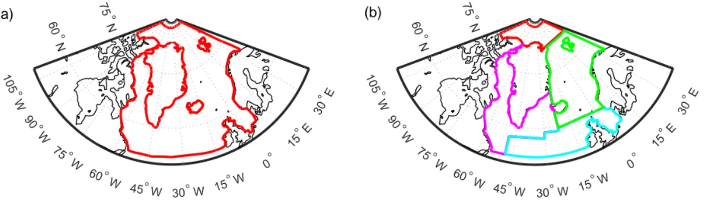
Figure 1.The 28-mascon parameterization of Greenland used in this study for GRACE data processing. For the purpose of further analysis, these patches are merged into five drainage systems (N, NE, SE, SW, and NW). Nine mascons (filled in blue) outside Greenland are added to absorb signals from the surrounding areas. Fifty-five glaciers utilized to compute seasonal ice discharge variations are marked in red. GRACE-based estimates, we limit the considered time
inter-val to January 2003–December 2013. Since data for 9 months are missing, 123 months in total are used. Furthermore, a re-duced time interval (January 2003–December 2012) is also considered in order to make the obtained estimates consis-tent with ice discharge data from Enderlin et al. (2014); see Sect. 2.3 for a further discussion. Due to strong noise in the C2,0 coefficients, we replaced them with available
esti-mates based on satellite laser ranging (Cheng et al., 2013). The degree-one coefficients, which are not included in the GRACE products, are taken from Swenson et al. (2008). The GRACE solutions are corrected for GIA, which is triggered by a relief of ice load since the Last Glacial Maximum, with the model from A et al. (2013).
To estimate mass variations over Greenland at a regional scale, we make use of a novel data processing methodology (Ran et al., 2018b), which is based on the mascon approach. Greenland is split into 28 patches, or “mascons” (Fig. 1), which are complemented by nine patches outside Greenland to absorb signals from the surrounding areas. Temporal vari-ations (anomalies) of surface density (i.e., mass varivari-ations per unit area) within each patch are assumed to be spatially homogeneous. Thus, the total mass anomaly within each patch is just a product of surface density anomaly and patch area. Those mass anomalies are computed for each month independently, without any regularization. Ultimately, mass anomalies are summed up over individual drainage systems or the entirety of Greenland.
A further description of the adopted GRACE data process-ing methodology is provided in the Appendix A. In order to investigate the robustness of GRACE-based mass anomalies, we estimate them using different processing parameters. This leads to multiple sets of GRACE solutions: two primary ones
(estimated with and without applying data weighting) and al-ternative ones. We also consider the estimates produced by other research teams: the Jet Propulsion Laboratory (JPL) mascon solutions by Watkins et al. (2015), the CSR mascon solutions by Save et al. (2016), the Goddard Space Flight Center (GSFC) mascon solutions by Luthcke et al. (2013), and the solutions by Wouters et al. (2008).
Similar to van den Broeke et al. (2009), we aggregate the 28 mascons inside Greenland into five drainage systems. We refer to these drainage systems as (a) north (N), (b) northwest (NW), (c) southeast (SE), (d) southwest (SW), and (e) north-east (NE) (Fig. 1). We slightly shifted southwards the bor-der between NW and SW drainage systems as compared to van den Broeke et al. (2009), in order to ensure that the SW drainage system is mostly limited to land-terminating glaciers.
2.2 SMB modeling
SMB values over 2003–2013 from three models (i.e., RACMO2.3, SNOWPACK, and MAR3.9) are analyzed. The SMB estimates are obtained as the sum of individual SMB components:
SMB = Ptot−SUtot−ERds−RU, (2) where Ptotand SUtotare the total precipitation and
sublima-tion, respectively; ERdsis erosion/deposition due to drifting
snow; and RU is runoff. The units are mass per unit time. The SMB mass anomalies used in this study are from RACMO2.3 unless stated otherwise. The output from SNOWPACK is in-cluded to evaluate the robustness of our findings with re-spect to the choice of SMB outputs simulated by different snow/firn models. Output of another regional climate model,
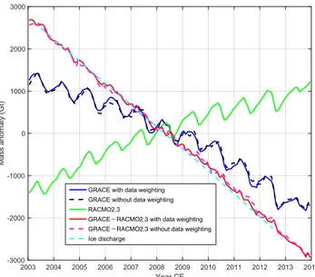
2003 2004 2005 2006 2007 2008 2009 2010 2011 2012 2013 2014 Year CE -3000 -2000 -1000 0 1000 2000 3000 Mass anomaly (Gt)
GRACE with data weighting GRACE without data weighting RACMO2.3
Ice discharge
Figure 2.Time series of mass anomalies over the period 2003–2013 for the entire GrIS: total mass anomalies from GRACE produced with and without data weighting (solid blue and dashed black, re-spectively), cumulative SMB anomalies from RACMO2.3 (green), the difference between them, the “total–SMB” residuals (solid red and dashed pink: with and without data weighting, respectively), and cumulative ice discharge (cyan).
MAR3.9, is also investigated in this study to demonstrate the robustness of the results, considering the large discrepancies among SMB outputs from different regional climate models in the past (Vernon et al., 2013).
2.2.1 RACMO2.3
RACMO2.3 was developed by the Royal Netherlands Mete-orological Institute (KNMI) and Institute for Marine and At-mospheric Research (IMAU), which is a part of Utrecht Uni-versity in the Netherlands (Noël et al., 2015). RACMO2.3 provides daily SMB values with a spatial resolution of 11 km. 2.2.2 SNOWPACK
In addition to the daily SMB provided by RACMO2.3, we use SMB output from SNOWPACK (Steger et al., 2017). SNOWPACK is a state-of-the-art snow model that offers a more physically based snow densification scheme, the simu-lation of microstructural snow properties, and a higher near-surface vertical resolution compared with the snow/firn mod-ule of RACMO2.3. A comparison of SNOWPACK with IMAU-FDM, a snow/firn model nearly identical to the one implemented in RACMO2.3, revealed a better performance of SNOWPACK for the GrIS, particularly for locations with comparably high amounts of liquid water input due to snowmelt and rainfall (Steger et al., 2017). SNOWPACK was coupled offline to RACMO2.3 and run for the full pe-riod 1960–2014 with the same surface mask (ocean,
tun-dra, ice sheet) and horizontal resolution as RACMO2.3. As a consequence of forcing SNOWPACK with mass fluxes from RACMO2.3 at the snow–atmosphere interface, differences in the simulated SMB from SNOWPACK and RACMO2.3 are thus only caused by unequal partitioning of meltwater and rainfall into refreezing and runoff.
2.2.3 MAR3.9
The MAR3.9 model was developed by the Laboratory of Climatology at the Department of Geography, University of Liège (Fettweis et al., 2017). It provides daily SMB val-ues for both the ice sheet and tundra areas with a spatial resolution of 5 km and uses ERA-Interim as forcing like RACMO2.3. The only differences between the version 3.8 of MAR used in Delhasse et al. (2018) and the version 3.9 used here are improvements in the MAR stability when it is applied at high resolution as well as in its computational ef-ficiency.
2.2.4 Processing the SMB outputs from RACMO2.3, SNOWPACK, and MAR3.9
In this study, we integrate SMB outputs from RACMO2.3, SNOWPACK, or MAR3.9 in time, which results in cumu-lative values that can be interpreted as daily SMB mass anomalies. These values are averaged over monthly inter-vals for the sake of temporal consistency with the GRACE solutions. In order to make the SMB outputs (11 km resolu-tion for RACMO2.3 and SNOWPACK, or 5 km in the case of MAR3.9) spatially match the GRACE resolution (around 300 km), we process them consistently with the GRACE data. This scheme is similar to the GRACE-like process-ing of SMB data by Alexander et al. (2016) and Velicogna et al. (2014). More specifically, we convert the SMB out-puts to gravity disturbances at the satellite altitude and limit their spectra to spherical harmonic degree/order 96. Then the SMB per mascon is estimated by a least-squares adjustment (see the Appendix A).
Previous studies on the sources of current GrIS mass loss used relative SMB outputs, i.e., anomalies with respect to an equilibrium state (1961–1990) (van den Broeke et al., 2009; Velicogna et al., 2014). Effectively, this means that the time series of mass anomalies were de-trended to ensure that they are close to zero during the reference equilibrium period. In other words, it assumes that the ice discharge and SMB were balanced during the reference period. In contrast, we use time series of absolute SMB mass anomalies, i.e., without refer-ring to a hypothesized equilibrium state. In this way, we are able to extract more information from the data sets: absolute mass anomalies related to ice discharge (i.e., the difference between GRACE- and SMB-based mass anomalies) cannot increase over time, which is a valuable constraint that facili-tates the correct interpretation of the obtained results.
Month -400 -300 -200 -100 0 100 200 300 400
Mean mass variation (Gt)
D J F M A M J J A S O N D
GRACE - RACMO 2.3 RACMO 2.3 GRACE
Figure 3. Greenland mean annual cycle of total mass anomalies from GRACE produced with data weighting (dark-blue), cumu-lative SMB anomalies (green), and the difference between them (brown) for the period 2003–2013. The latter curve reflects the cu-mulative sum of seasonal ice discharge variations and meltwater storage, as well as GRACE errors and SMB model bias. The shaded strips show the 1σ error bars. Labels at the horizontal axis indicate month of the year (e.g., month “J” denotes January, while month “D” is December).
2.3 Ice discharge
We examine ice discharge from two different data sets. The first set was presented in Enderlin et al. (2014). Here, it is used to reconstruct the 2003–2012 multi-year mass trends and accelerations, as well as to separate the contributions from SMB and ice discharge. It covers 178 outlet glaciers with annual resolution. Ice discharge observations of these glaciers are estimated by multiplying ice flow velocities with ice thickness values. Annual velocities are retrieved by means of feature tracking from (winter) Landsat 7 En-hanced Thematic Mapper Plus and the Advanced Spaceborne Thermal and Reflectance Radiometer (ASTER) data. Ice dis-charge is calculated within 5 km of the grounding lines. The ice thicknesses at the flux gates are computed by subtract-ing bed elevations from surface elevations. Bed elevations are derived from NASA’s Operation IceBridge airborne ice-penetrating radar data, whereas surface elevations are ob-tained from digital elevation models (Enderlin et al., 2014; Xu et al., 2015).
In addition, we produce the second data set, which is used to examine monthly variations of ice discharge. It covers 55 marine-terminating glaciers with sub-annual resolution for 2009–2013. The exploited ice flow velocities were ob-tained from TerraSAR-X images delivered by DLR (Moon et al., 2014). Ice thicknesses at the flux gates are interpo-lated from the IceBridge BedMachine Greenland version 2 data (Morlighem et al., 2015). Ice discharge (D) for a given
glacier is defined as the ice mass flux across the flux gate (f ) close to the glacier terminus (within ∼ 5 km):
D = ρ Z
h(υ · n)df, (3)
where h is the ice thickness, n is the unit vector directed out-wards normally to the flux gate, υ is the ice flow velocity, and ρ is the ice density. When selecting flux gates, we pay attention to variations of the terminus position by checking the images of glaciers during the whole time interval, to make sure that the flux gate is upstream of the terminus all the time. Furthermore, a flux gate should span the whole outlet glacier to the ice flow edges. To compute D, we discretize the flux gates into nearly 200 m long intervals. The length of the last interval is adjusted to make sure that the ice flow edge is sampled. We then use the values (h, υ, and n) defined for the center of each interval, assuming that they are constant over the interval. Then Eq. (3) becomes
D = ρ
N
X
i=1
dihi(υi·n), (4)
where N is the total number of intervals of the flux gate and di is the length of the ith interval.
3 Results and discussion
3.1 Multi-year mass trend and acceleration budgets First, we examine multi-year mass trends and accelerations in terms of the total mass balance and the contributions thereto from SMB and ice discharge. For more details about the estimation of multi-year trend and accelerations, please refer to Appendix B.
Our estimate of the total-mass linear trend, which is based on the primary GRACE data time series produced with op-timal data weighting, is −286 ± 21 Gt yr−1 for 2003–2013.
The estimate obtained without data weighting is −279 ± 21 Gt yr−1. The individual contributors to the errors in the
trend estimates are shown in Table A1. Our estimates are in agreement with those published earlier for the time interval 2003–2013: −280 ± 58 Gt yr−1(Velicogna et al., 2014) and
−278 ± 19 Gt yr−1(Schrama et al., 2014).
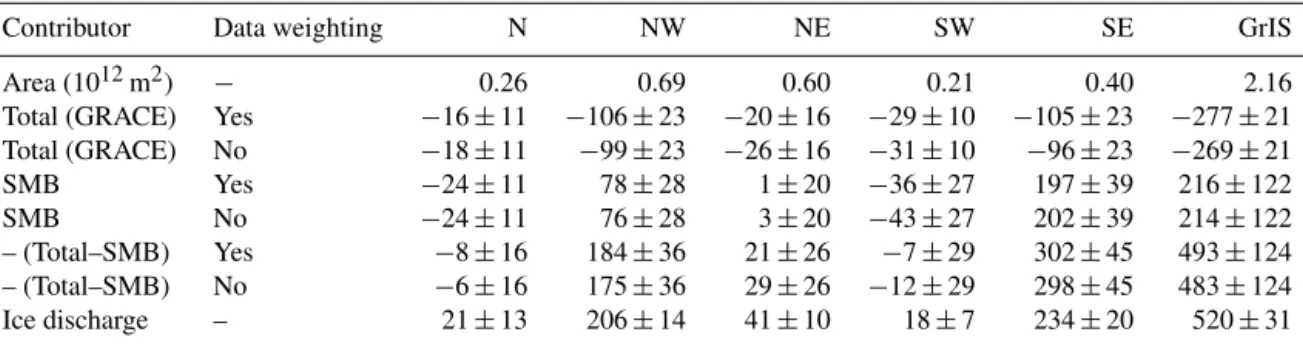
We also examine the SMB and ice discharge contribu-tions to the total mass trend. In this case, we consider the reduced time interval, 2003–2012, in order to be consistent with the ice discharge record, which ends in 2012 (Table 1). The multi-year average mass gains from SMB (RACMO2.3) over that period processed consistently with GRACE via data weighting and without data weighting are 216 ± 122 and 214±122 Gt yr−1, respectively. The uncertainty is computed
by assuming a 9 % error in accumulation and a 15 % error in meltwater runoff signals modeled by RACMO2.3, which is the typical uncertainty of RACMO2.3 (van den Broeke
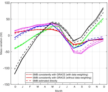
Month -150 -100 -50 0 50 100 Mass variation (Gt) D J F M A M J J A S O N D
SMB consistently with GRACE (with data weighting) SMB consistently with GRACE (without data weighting) SMB estimated directly
Figure 4.Similar to Fig. 3, but only for mean annual cycle of cu-mulative SMB anomalies of different drainage systems (SE: black; NW: green; NE: blue; N: red; SW: pink). The SMB outputs are computed in three different ways: (i) consistently with GRACE data (with or without data weighting) and (ii) by a direct estimation of mass anomalies per drainage system.
et al., 2016). The time series of cumulative mass anomalies due to ice discharge and other processes not related to SMB is obtained as the difference between the total mass varia-tions and the cumulative SMB-related ones; this difference will be referred to as the “total–SMB” residuals (“total mi-nus SMB”; cf. red and pink curves in Fig. 2). The associated rates of linear changes over 2003–2012 estimated with and without data weighting are 493±124 and 483±124 Gt yr−1,
respectively. Those estimates agree with the ice discharge es-timate from Enderlin et al. (2014), 520 ± 31 Gt yr−1, shown
as the cyan curve in Fig. 2, which is shifted to best fit the GRACE-SMB time series. Notice that the GRACE time se-ries obtained with the optimal weighting shows a smoother behavior than that produced without data weighting. This is consistent with the analysis presented in Ran et al. (2018a, b), who found that data weighting substantially reduces the level of random noise in the GRACE GrIS mass change time series.
Next, we present the results of a similar analysis for the in-dividual drainage systems. The greatest total mass losses are observed by GRACE in drainage systems NW and SE (cf. Fig. A2 and Table 1). These two drainage systems account for ∼ 73–76 % of the total mass loss over Greenland, depend-ing on whether data weightdepend-ing is applied or not. The interan-nual behavior of these drainage systems is, however, differ-ent. SE loses mass with an approximately constant rate over the whole considered period. In contrast, NW is relatively stable over the period 2003–2005, but starts losing mass thereafter. The remaining three drainage systems lose mass
at much smaller rates. Remarkably, two of these drainage systems (N and SW) show a similar behavior: they are rela-tively stable over the period 2003–2009 but start losing mass in 2010. These findings are consistent with Velicogna et al. (2014). The SMB is negative in two drainage systems (N and SW) (cf. Table 1). However, with a large fraction of land-terminating glaciers, ice losses from ice discharge are an or-der of magnitude lower there than in the NW and SE drainage systems (cf. Fig. A2), resulting in only modest total mass loss in spite of the negative SMB.
The long-term trends of total–SMB residuals in the drainage systems of NW, NE, and SW are consistent with the ice discharge estimates from Enderlin et al. (2014) within the error bar (Table 1). This suggests robustness of RACMO2.3 long-term SMB trends there, under the assumption that the meltwater storage signal is mainly seasonal. In the SE and N, however, we find relatively large discrepancies between the total–SMB residuals and ice discharge observations from En-derlin et al. (2014). Under the conditions of realistic GRACE error estimates and minimal multi-year meltwater storage, all these inconsistencies suggest a precipitation overestimation in the SE and underestimation in the N in RACMO2.3.
Average accelerations of mass change anomalies over the period 2003–2012 are also estimated using Eq. (B1) (param-eter a3). Over the entirety of Greenland, the SMB (−23.3 ±
2.7 Gt yr−2) contributes 75 % of the total acceleration
ob-served by GRACE (Table A2). This is close to the estimates of Velicogna et al. (2014), who assessed the contribution of SMB to the total GrIS mass loss acceleration as 79 %. The contribution of the total–SMB residuals to the mass loss ac-celeration for the entirety of Greenland is statistically in-significant. Analysis of individual drainage systems leads to similar conclusions (cf. Table A2). However, we note that the acceleration estimates cannot be simply extrapolated onto a longer time interval and may not properly represent the ice sheet behavior at the decadal timescale, because of the large climate variability in a limited time span of data (Wouters et al., 2013).
3.2 Seasonal mass variations
We analyze the mean annual cycles of total (GRACE) and cumulative SMB (RACMO2.3) mass anomalies over the pe-riod 2003–2013 (Fig. 3). To derive them, we divide the entire period into 11 overlapping 13-month time intervals, each of which starts in December of the previous year and ends in December of the current year. Then, the mean mass anomaly for each calendar month is estimated by linear regression, together with one bias parameter per time interval, which ac-counts for a long-term variability. This scheme is less sen-sitive to gaps in data time series than the plain averaging of mass anomalies per calendar month. For more details about this scheme, we refer the reader to Ran et al. (2018a). The un-certainties of mean mass anomalies from GRACE are prop-agated from errors in each monthly GRACE estimate. The
Month
-200 0 200 400
(a) Mass variation (Gt) D J F M A M J J A S O N D
Month 0 50 100 (b) Mass variation (Gt) D J F M A M J J A S O N D N NW SE NE Month 0 0.1 0.2 (c) EWH (m) D J F M A M J J A S O N D N NW SE NE
Figure 5.Mean monthly meltwater production per calendar month (gigatonnes) for the entirety of Greenland (a), for individual drainage systems in gigatonnes (b), and for individual drainage systems in meters of equivalent water height (c) modeled by RACMO2.3.
Table 1.Linear mass change rates over the period 2003–2012 for individual drainage systems and the entirety of Greenland: total, SMB-related, and total–SMB residuals (GRACE–SMB), as well as ice discharge (Gt yr−1). The sign of total–SMB residuals is changed to make
them directly comparable with ice discharge estimates.
Contributor Data weighting N NW NE SW SE GrIS
Area (1012m2) − 0.26 0.69 0.60 0.21 0.40 2.16
Total (GRACE) Yes −16 ± 11 −106 ± 23 −20 ± 16 −29 ± 10 −105 ± 23 −277 ± 21 Total (GRACE) No −18 ± 11 −99 ± 23 −26 ± 16 −31 ± 10 −96 ± 23 −269 ± 21 SMB Yes −24 ± 11 78 ± 28 1 ± 20 −36 ± 27 197 ± 39 216 ± 122 SMB No −24 ± 11 76 ± 28 3 ± 20 −43 ± 27 202 ± 39 214 ± 122 – (Total–SMB) Yes −8 ± 16 184 ± 36 21 ± 26 −7 ± 29 302 ± 45 493 ± 124 – (Total–SMB) No −6 ± 16 175 ± 36 29 ± 26 −12 ± 29 298 ± 45 483 ± 124 Ice discharge – 21 ± 13 206 ± 14 41 ± 10 18 ± 7 234 ± 20 520 ± 31
uncertainties of cumulative SMB mean mass anomalies are computed by assuming 9 % and 15 % errors in modeled mean mass anomalies due to precipitation and runoff, respectively, as suggested by van den Broeke et al. (2016). The uncertain-ties of the total–SMB residuals are the mean root sum square of the standard deviations of noise in GRACE and cumula-tive SMB estimates.
The whole-Greenland mean annual cycles of total and cu-mulative SMB mass anomalies present smooth month-to-month variations (Fig. 3). Importantly, the estimates of both types refer to the mean values for the months considered. The total mass anomaly from GRACE reaches its maximum in March and then steadily decreases until September. The most rapid monthly mass loss is observed in July–August
(∼ 200 Gt). In contrast, the cumulative SMB decreases over a much shorter period – only from May to August.
Alexander et al. (2016) suggested that the inconsistency between the spatial resolution of GRACE-based estimates and that of the SMB model (11 km) may have a large impact on the difference between the two time series. In response to this concern, we investigate the effect of using an alternative scheme to process SMB mass anomalies. Instead of process-ing them consistently with GRACE data, as was explained in Sect. 2.2.4, we directly compute SMB-related mass anoma-lies per drainage system from the RACMO2.3 grid with a spatial resolution of 11 km. We find that the difference for the entirety of Greenland is negligible: smaller than 2 Gt. For individual drainage systems, we find that the impact is also
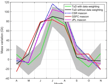
Month -40 -20 0 20 40 60 80 100 120 Mass variation (Gt) A M J J A S O N
TuD with data weighting TuD without data weighting CSR mascon
GSFC mascon JPL mascon
Figure 6.Estimates of seasonal meltwater storage, obtained as the monthly deviations from the April–May and September–November linear fit of “total–SMB” residuals (brown line in Fig. 3): for the whole GrIS (in gigatonnes). Labels along the horizontal axis repre-sent months between April (“A”) and November (“N”). The shaded strip shows the 1σ error bar for the estimates by Delft University of Technology (TuD) with data weighting (the mean standard devi-ation is 23 Gt).
relatively small (< 12 Gt, which is around 10 % of the signal) (see Fig. 4). Still, this effect shows a systematic behavior and may introduce some bias into GRACE-SMB estimates. For this reason, we prefer to process SMB estimates consistently with GRACE data (Alexander et al., 2016; Velicogna et al., 2014).
3.2.1 A simple method of quantifying short-term meltwater storage
The total–SMB residuals show some periods of almost null variations (nearly flat segments in Fig. 3): February–March, May–July, and November–December. The total–SMB resid-uals represent the cumulative sum of ice discharge, meltwa-ter storage, GRACE errors, and SMB model biases. If we assumed that the main contributor to the total–SMB residu-als is ice discharge, these nearly flat features would indicate that ice discharge is negligible or even negative, which is un-physical, since this implies that discharge is contributing to Greenland mass gain. Therefore, these features should be ex-plained either by meltwater storage or by errors in SMB- and GRACE-based estimates. Based on the robustness analysis of the total–SMB estimates in Appendix C, we infer that the quasi-null total–SMB variations during February–March and November–December are likely caused by noise in the esti-mates. In the following, therefore, they will not be discussed. The summer flat feature of May–July, however, always per-sists, no matter what data processing scenario is followed.
Month 125 130 135 140 145 150 155 160 165 Ice discharge (Gt yr -1) J F M A M J J A S O N D 2009 2010 2011 2012 2013 (a) NW Month 108 110 112 114 116 118 120 Ice discharge (Gt yr -1) J F M A M J J A S O N D 2009 2010 2011 2012 2013 (b) SE Month 240 245 250 255 260 265 270 275 280 285 Ice discharge (Gt yr -1) J F M A M J J A S O N D 2009 2010 2011 2012 2013 (c) NW and SE
Figure 7.Monthly ice discharge estimates from 55 major marine-terminating glaciers for the glaciers in the NW drainage system (a)and the SE drainage system (b) individually, and for the NW and SE drainage systems together (c).
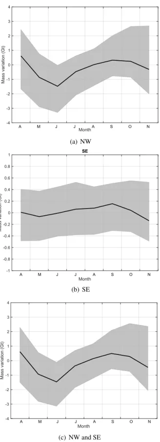
Month -4 -3 -2 -1 0 1 2 3 4 Mass variation (Gt) A M J J A S O N (a) NW Month -1 -0.8 -0.6 -0.4 -0.2 0 0.2 0.4 0.6 0.8 1 Mass variation (Gt) SE A M J J A S O N (b) SE Month -4 -3 -2 -1 0 1 2 3 4 Mass variation (Gt) A M J J A S O N (c) NW and SE
1
Figure 8.Similar to Fig. 6 but for mean ice-discharge-related vari-ations over 2009–2013. The cumulative mass anomalies are com-puted from glaciers in NW (a) and SE (b) drainage systems indi-vidually, and for glaciers in NW and SE together (c).
Thereby, we suggest that it is attributed to a physical signal, i.e., short-term meltwater storage.
Hereafter, we propose a simple method with which to elu-cidate and quantify short-term meltwater storage. According to RACMO2.3, meltwater is mostly produced between May and September, and peaks in July (cf. Fig. 5). Averaged over the GRACE period, approximately 800 Gt of meltwater is produced on average in Greenland during the melt season from May to September, of which ∼ 250 Gt is estimated to refreeze within the snowpack, and the rest runs off of the ice sheet. RACMO2.3 does not calculate lateral meltwater transport, i.e., the time lag between meltwater production and the moment when the runoff reaches the ocean. During late spring and early summer, this lag is particularly significant due to an inefficient subglacial channelized network (Renner-malm et al., 2013) and replenishing of firn aquifers (mainly in the SE and NW) (Forster et al., 2014; Miège et al., 2016). In order to estimate the instantaneous amount of meltwa-ter subject to runoff, we first fit the total–SMB residuals in two periods, before and after the flat feature (i.e., in April– May and September–November), with a linear function. This function can be interpreted as an empirical estimation of the mean combined effect of ice discharge and the difference be-tween the modeled meltwater refreezing and the actual one. Then, we force the mass budget at the beginning and the end of the melt season to be closed by subtracting the obtained linear function from the total–SMB residuals (Fig. 6). In this way, we find that meltwater is retained in Greenland between May and October, with a 100±20 Gt maximum in July. Note that the estimates of meltwater storage are sufficiently ro-bust with respect to the choice of the GRACE-based mascon solution, but they may vary in a small range in timing and amplitude (Fig. 6). The uncertainties of meltwater storage are computed as the root sum square of the standard devi-ations of noise in GRACE- and SMB-based estimates. It is worth mentioning that the error in the SMB estimates is then computed assuming 9 % and 15 % errors in modeled mean mass anomalies due to precipitation and runoff signals, re-spectively, after applying the same linear regression function (see above) to each component.
Estimates of non-SMB mass anomalies could reflect the delayed release of meltwater into the ocean and the vari-ability of ice discharge. We test the effects of ice discharge variability using a monthly resolved data set of ice discharge for 55 glaciers in Greenland (See Fig. 1). These glaciers are largely located in the NW and SE Greenland drainage sys-tems, which are the largest contributors of ice mass wastage into the ocean. The sum of the obtained estimates over all 55 glaciers is shown in Fig. 7a. One can see that at the whole-ice-sheet scale the increase in ice discharge during the melt season is minor in all years (∼ 10 % or less). In the absence of complete coverage of the GrIS with observations of glacier velocities at the seasonal timescale, we compute a scale fac-tor as the ratio between the ice discharge estimates from 55 glaciers considered in this study and the discharge over the
Month -20 0 20 40 Mass variation (Gt) NW A M J J A S O N
TuD with data weighting TuD without data weighting CSR mascon GSFC mascon Month -20 0 20 40 Mass variation (Gt) SE A M J J A S O N Month 0 10 20 Mass variation (Gt) N A M J J A S O N
Figure 9.Similar to Fig. 6, but the estimates of seasonal meltwater storage are extracted from different mascon solutions for individual drainage systems: NW, SE, and N. The errors are not shown in the plot for the sake of its readability. The mean standard deviations of the errors for NW, SE, and N are 25, 26, and 9 Gt, respectively.
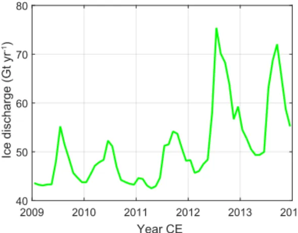
Year CE 2009 2010 2011 2012 2013 2014 Ice discharge (Gt yr -1) 40 50 60 70 80
Figure 10. Monthly variations of ice discharge of Jakobshavn Glacier over the period 2009–2013 (Gt yr−1).
entire GrIS in terms of the long-term linear trend by Enderlin et al. (2014), and apply this scale factor (i.e., ∼ 2) to the ice discharge estimate of each glacier. Then, similar to Fig. 6, we represent the ice discharge related mean mass anomaly per calendar month in terms of the deviation from the lin-ear function fitting the values in April–May and September– November (cf. Fig. 8c). One can see that the effect of ice dis-charge amounts to only a few gigatonnes; i.e., its contribution to the total signal is negligible. This supports our hypothesis
that that delayed runoff is likely the major contributor to the signal isolated in Fig. 6.
Finally, we examine individual drainage systems (cf. Figs. 9 and A6). We refrain from an analysis of the SW and NE regions due to a relatively high level of noise in the ob-tained meltwater storage estimates. Regionally, the SE shows the largest meltwater accumulation per unit area. This is con-sistent with the fact that the rate of meltwater production is large in the sector (Fig. 5), as is the storage potential owing to high accumulation rates (Miège et al., 2016). In the N and NW regions, the signal related to meltwater storage is less pronounced, which can be explained by the dry climate of this region, meaning that less pore space is available in the firn layer to store liquid water.
In terms of the total mass, the largest meltwater accumula-tion takes place in the NW and SE regions: the contribuaccumula-tion of each region may reach around 40 Gt in July–August (cf. Figs. 9 and A6).
As for the increase in ice discharge during the melt sea-son, we find that it is relatively minor for both NW and SE drainage systems (less than 20 % and 10 %, respectively; see Fig. 7). As such, the contribution of ice discharge to the sig-nal reported in Figs. 9 and A6 is minor for both drainage systems: not more than 2.0 ± 1.9 and 0.3 ± 0.5 Gt, respec-tively (cf. Fig. 8). Interestingly, a much larger increase in ice discharge during the melt season is found for the single ma-jor contributor to ice discharge, Jakobshavn Glacier: up to
60 % in 2012 (Fig. 10). This finding is consistent with that of Joughin et al. (2008, 2012).
Note that the meltwater storage signal at the drainage sys-tem scale is present in all GRACE mascon solutions but shows some discrepancies in the timing and amplitude. This means that further effort is still needed to improve the accu-racy of GRACE-based estimates.
4 Conclusions
GRACE monthly solutions have been applied to systemati-cally analyze the mass budget in the territory of Greenland at various temporal and spatial scales. The obtained estimate of the mean rate of mass loss produced from CSR RL05 solu-tions with the new variant of the mascon approach with and without data weighting is −277 ± 21 and −269 ± 21 Gt yr−1
over the period 2003–2012, respectively. The rate of SMB ac-cumulation, as modeled by RACMO2.3 and processed con-sistently with GRACE data, is 216 or 214 ± 122 Gt yr−1,
de-pending on whether data weighting is applied or not. The dif-ferences between GRACE- and RACMO-based trends with or without data weighting are 493±124 or 483±124 Gt yr−1,
which are consistent with 2003–2012 ice discharge observa-tions by Enderlin et al. (2014): 520±31 Gt yr−1. On the other
hand, we observe relatively large discrepancies between the estimates for the SE and N drainage systems. Those discrep-ancies imply that the adopted climate model likely overesti-mates precipitation in the SE drainage system and underesti-mates it in the N drainage system.
Our estimates of accelerations in SMB-related (−23.3 ± 2.7 Gt yr−2), ice discharge-related (2.6 ± 1.5 Gt yr−2), and
total (−31.1 ± 8.1 Gt yr−2) mass anomalies are consistent
within error bars. Most of the observed acceleration in mass loss can be attributed to changes in SMB. This is consis-tent with Velicogna et al. (2014), who found that 79 % of the mass loss acceleration can be explained by the contribu-tion of SMB. Furthermore, our results indicate that most of the total mass acceleration observed by GRACE is attributed to the SW and NW drainage systems, which is in agreement with Velicogna et al. (2014).
We found a remarkable seasonal cycle in the difference between monthly total and SMB cumulative mass anoma-lies (“total–SMB” residuals), which likely reflects significant meltwater storage in the early summer months due to an in-efficiency of the subglacial channelized network. The maxi-mum storage is observed in July: 80–120 Gt. To estimate the potential contribution of ice discharge to the observed sig-nals, we exploited the estimates of ice discharge over 55 out-let glaciers obtained with the flux gate method. We showed that seasonality in ice discharge is on the order of a few gi-gatonnes; i.e., it is negligible compared with meltwater stor-age. We also analyzed the short-term meltwater storage per drainage system. Our results suggest that the meltwater stor-age is large in NW and SE drainstor-age systems, whereas it is weak in the northern drainage system.
A comparison of estimates derived from GRACE data with different processing parameters and from different mascon products (e.g., JPL, CSR, and GSFC) revealed the presence of the short-term meltwater storage signal in all the consid-ered solutions. At the same time, noticeable discrepancies are observed in timing and amplitude in meltwater storage estimates. These indicates that further work is needed to im-prove GRACE-based estimates at both Greenland-wide and drainage system scales.
Finally, this work illustrates the potential of combining multiple observational data sets and model output com-plemented by simple physical constraints, to better under-stand the contributors to GrIS mass variations at various timescales. Improving the estimates of (natural and forced) mass variations associated with individual processes is im-portant for robust projections of future GrIS evolution and its contribution to sea level rise.
Data availability. GRACE Level 2 data and the corresponding er-ror variance–covariance matrices used in this study are provided by the Center for Space Research at the University of Texas at Austin. The mascon product estimated by the optimal data weight-ing scheme is available from the authors unconditionally.
Appendix A: Adopted method for estimating mass variation from GRACE
Our GRACE-based estimates of total mass variations are derived using a new variant of the mascon approach (Ran, 2017). The method is adapted from the computational proce-dures proposed by Forsberg and Reeh (2007) and Baur and Sneeuw (2011). The procedure consists of two steps: (1) syn-thesizing temporal variations of gravity disturbances at a set of data points located at a specific satellite altitude (500 km). The data points are homogeneously distributed over Green-land (extended with a 800 km buffer zone) with a 37.5 km separation. The full error covariance matrix Cd of the
grav-ity disturbances is computed on the basis of the full er-ror covariance matrix of the spherical harmonic coefficients. (2) The synthesized gravity disturbances are converted into mass anomalies per patch. The procedure is based on a linear functional model:
d = Ax + n, (A1)
where d is a vector composed of synthesized gravity distur-bances, x is the vector consisting of mass anomalies, A is the design matrix relating the two vectors to each other in line with Newton’s attraction law, and n is the data noise vector. A straightforward implementation of this functional model may lead to some additional errors due to a spectral incon-sistency between the matrix A and the data vector d. The ith column of A can be interpreted as a set of gravity dis-turbances caused by a unit mass anomaly in the ith patch; its spatial spectrum is unlimited. The spatial spectrum of gravity disturbances d is limited to the maximum degree of the input spherical harmonic coefficients (here, 96). We eliminate this inconsistency by a low-pass filtering of all the columns of the matrix A, so that the contribution of the spherical harmonics above degree 96 is suppressed. The mass anomalies are com-puted from gravity disturbances by means of a least-squares adjustment: 105 ° W 90 ° W 75 ° W 60° W 45° W 30° W 15 ° W 0 ° 15 ° E 30 ° E 60 ° N 75 ° N 105 ° W 90 ° W 75 ° W 60° W 45° W 30° W 15 ° W 0 ° 15 ° E 30 ° E 60 ° N 75 ° N (a) (b)
Figure A1.Parameterization of the ocean area around Greenland with one (a) and four (b) patches.
x = (ATPA)−1ATPd, (A2)
where P is the weight matrix computed by an approximate in-version of the error covariance matrix of gravity disturbances Cd. The exact inverse of Cdcannot be computed because the
matrix Cd is ill posed. Therefore, an approximate inversion
of Cdis introduced, which is based on the eigenvalue
decom-position of Cd; only a limited number of the largest
eigenval-ues are retained. The usage of the matrix P ensures a (nearly) statistically optimal data weighting. From a preliminary nu-merical study we found that the optimal choice is to retain 600 eigenvalues. No spatial regularization is applied in the course of inversion.
This procedure is used to produce one of the primary solu-tions, referred to as the “solution obtained with data weight-ing”; the other primary solution, referred as the “solution ob-tained without data weighting”, is produced with the ordinary least-squares adjustment
2004 2006 2008 2010 2012 2014 -200 0 200 N 2004 2006 2008 2010 2012 2014 -2000 -1000 0 1000 2000 Mass anomaly (Gt) NW 2004 2006 2008 2010 2012 2014 Year CE -200 0 200 SW 2004 2006 2008 2010 2012 2014 -2000 -1000 0 1000 2000 SE GRACE RACMO2.3 2004 2006 2008 2010 2012 2014 -200 0 200 NE
Figure A2.Same as Fig. 2 but for the GRACE-based estimates produced with data weighting at the drainage system scale. The estimates produced without data weighting are not shown as they are very similar to those with data weighting.
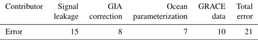
Table A1.Contribution of different error sources to the error in the total GrIS mass trend estimated from GRACE data both with and without data weighting (in Gt yr−1).
Contributor Signal GIA Ocean GRACE Total
leakage correction parameterization data error
Month -400 -300 -200 -100 0 100 200 300 400
Mean mass variation (Gt)
D J F M A M J J A S O N D
TuD with data weighting TuD without data weighting 200 eigenvalues 400 eigenvalues One ocean mascon Four ocean mascons Degree-1 by Sun et al., (2016) Degree-1 by Cheng et al., (2013)
Figure A3. The mean mass anomalies per calendar month of the total–SMB residuals over the entirety of Greenland estimated by applying different GRACE data processing schemes.
Month -400 -300 -200 -100 0 100 200 300 400
Mean mass variation (Gt)
D J F M A M J J A S O N D
TuD with data weighting TuD without data weighting BW
CSR mascon JPL mascon GSFC mascon
Figure A4. The mean mass anomalies per calendar month of the total–SMB residuals over the entirety of Greenland estimated from different GRACE solutions. “BW” refers to the solution of Wouters et al. (2008). Month -400 -300 -200 -100 0 100 200 300 400
Mean mass variation (Gt)
D J F M A M J J A S O N D
Figure A5.The mean mass anomalies per calendar month of the total–SMB residuals over the entirety of Greenland estimated from different SMB outputs.
Month -0.02 0 0.02 0.04 0.06 EWH (m) NW A M J J A S O N
TuD with data weighting TuD without data weighting CSR mascon GSFC mascon Month 0 0.05 0.1 EWH (m) SE A M J J A S O N Month 0 0.05 0.1 EWH (m) N A M J J A S O N
Figure A6.Similar to Fig. 9 but in meters of equivalent water height. The mean standard deviations of the errors for NW, SE, and N are 0.04, 0.07, and 0.03 m, respectively.
Table A2.Acceleration of mass change over the period 2003–2012 for individual drainage systems and the entirety of Greenland: total, SMB-related, and total–SMB residuals (GRACE minus SMB), as well as ice discharge (Gt yr−2). The sign of total–SMB residuals is changed to
make them directly comparable with ice discharge estimates.
Contributor Data weighting N NW NE SW SE GrIS
Total (GRACE) Yes −2.9 ± 1.5 −15.6 ± 3.1 −1.1 ± 2.9 −10.9 ± 4.2 −0.7 ± 5.2 −31.1 ± 8.1 Total (GRACE) No −3.6 ± 1.5 −15.7 ± 3.1 −0.7 ± 2.9 −9.4 ± 4.2 −1.8 ± 5.2 −31.2 ± 8.1 SMB Yes −3.5 ± 0.4 −8.2 ± 1.1 −2.8 ± 0.2 −12.1 ± 0.9 3.3 ± 0.4 −23.3 ± 2.7 SMB No −3.4 ± 0.4 −8.5 ± 1.1 −2.3 ± 0.2 −14.6 ± 0.9 5.5 ± 0.4 −23.3 ± 2.7 – (Total–SMB) Yes −0.6 ± 1.6 7.4 ± 3.3 −1.7 ± 2.9 −1.2 ± 4.3 4.0 ± 5.2 7.8 ± 8.5 – (Total–SMB) No 0.2 ± 1.6 7.2 ± 3.3 −1.6 ± 2.9 −5.2 ± 4.3 7.3 ± 5.2 7.9±,8.5 Ice discharge – 0.5 ± 0.5 2.1 ± 0.7 0.2 ± 0.5 −0.1 ± 0.4 −0.1 ± 1.1 2.6 ± 1.5
Appendix B: The estimation of multi-year trend and acceleration
We approximate each mass anomaly time series (cf. Fig. 2) with the following analytic function:
f (t ) = a1+a2(t − t0) + a3(t − t0)
2
2 +a4sinωt + a5cosωt
+a6sin2ωt + a7cos2ωt, (B1)
where a1, . . . , a7 are parameters to be estimated; t0 is a
reference epoch defined as the middle of the considered time interval (i.e., 1 July 2008 for the time interval 2003– 2013; 1 January 2008 for the time interval 2003–2012); and ω =2π/T , with T = 1 year.
In addition, we calculate the uncertainty of the trend esti-mate, a2. This uncertainty of the GRACE-based estimate (see
Table A1) is composed of the error of the GIA model (we set it as 50 % of the signal; Jacob et al., 2012), the measure-ment errors of GRACE propagated from the full variance– covariance matrix of monthly solutions, the uncertainty as-sociated with a particular choice of the oceanic mascon lay-out (cf. Fig. A1), and signal leakage. The latter (including both signals which leaked from outside Greenland and sig-nals from inside Greenland which leaked between the mas-cons) was simulated numerically by defining the trend from ICESat as the reference. Note that the individual errors are summed up quadratically, by assuming that they are not cor-related with each other. We do not consider errors from at-mospheric and ocean circulation corrections, as the impact of those errors is negligible (Ran et al., 2018a, b). A similar approach is applied to estimate the uncertainty of accelera-tion (parameter a3).
Appendix C: Robustness of the total–SMB residuals at the seasonal timescale
In this section, we investigate the robustness of total–SMB residuals with respect to those errors. To assess a possi-ble impact of errors in GRACE-based mass anomalies, we try different processing schemes in our variant of the mas-con method. The following modifications of the GRACE data processing scheme were considered: (i) retaining a dif-ferent number of eigenvalues of the noise covariance ma-trix Cd when inverting this matrix within the frame of the
weighted least-squares estimation: 200, 400, or 600 eigen-values (600 eigeneigen-values is the primary option); (ii) differ-ent handling of the surrounding ocean: parameterization with one patch, parameterization with four patches (cf. Fig. A1), or without estimating mass anomalies over ocean (the latter is the primary option); and (iii) a different choice of spher-ical harmonic degree-one coefficients: from Swenson et al. (2008), Cheng et al. (2013), or Sun et al. (2016) (the for-mer is the primary option). Note that only one parameter
varies at a time, while the primary option is chosen to de-fine the other parameters (see also the Appendix A). The op-timal data weighting is exploited in all these experiments. In addition, we consider an effect of switching to the ordi-nary least-squares adjustment (when the data weighting is not used). We also consider alternative GRACE-based esti-mates: JPL mascon solutions by Watkins et al. (2015), CSR mascon solutions by Save et al. (2016), GSFC mascon so-lutions by Luthcke et al. (2013), and mascons soso-lutions of Wouters et al. (2008).
The results are depicted in Figs. A3–A4. The presence and appearance of the nearly zero total–SMB month-to-month variations during February–March and November– December vary between GRACE estimates. When the sur-rounding ocean is parameterized with four patches, the February–March feature becomes less flat; the November– December flat feature is not significant either in the estimates based on the ordinary least-squares estimator and on Wouters et al. (2008). In addition, the flat features of February–March and November–December do not appear in the total–SMB residuals obtained from the CSR and JPL mascon solutions. Therefore, we infer that the nearly zero total–SMB vari-ations during February–March and November–December, which are clearly visible in Fig. 3, are likely caused by noise in the GRACE-based estimates. In the following, therefore, they will not be discussed. On the other hand, the flat fea-ture of May–July persists, no matter what processing pa-rameters are chosen and which GRACE product is utilized. Therefore, it cannot be explained by uncertainties associated with GRACE data processing. Remarkably, switching data weighting on/off has the maximum impact on the obtained estimates of mass anomalies per calendar month. Since it is not clear at this moment which of the two options leads to better estimates, the results produced both without and with optimal data weighting will be considered in the further dis-cussion of the main text.
To assess a possible impact of uncertainties in the SMB output, we analyze the SMB mass anomalies from RACMO2.3, SNOWPACK, and MAR3.9. As shown in Fig. A5, the May–July flat feature persists in the total– SMB residuals estimated from RACMO2.3, SNOWPACK, and MAR3.9. Therefore, we conclude that the May–July flat feature is likely not triggered by noise in the SMB estimates. As such, it must be attributed to a physical signal. We suggest that this signal is caused by short-term meltwater storage.
Author contributions. PD, RK, and JR developed the methodology for GRACE data processing; JR processed the GRACE data; PD, MV, and JR interpreted the results based on GRACE data; MV ini-tiated their comparison with ice discharge data; JR, MV, and PD wrote the manuscript; MvdB, TM, EE, CRS, CHR, BW, XF, MZ, and LL provided additional data; BW contributed to the GRACE-intercomparison; and all authors commented on the manuscript.
Competing interests. The authors declare that they have no conflict of interest.
Acknowledgements. We thank the constructive and insightful comments by the editor, Joseph MacGregor, and two anonymous reviewers. Jiangjun Ran thanks his sponsor, the Chinese Schol-arship Council. Jiangjun Ran has also been partly supported by the National Natural Science Foundation of China (41474063, 41431070, and 41674084), the National Key Research and Development Program of China (2018YFC1406100), and the Strategic Priority Research Program of the Chinese Academy of Sciences (XDB23030100). Miren Vizcaino is funded by the Dutch Technology Fellowship. Michiel R. van den Broeke and Bert Wouters acknowledge funding from the Polar Programme of the Netherlands Organization for Scientific Research (NWO/NPP) and the Netherlands Earth System Science Centre (NESSC). Lin Liu is funded by the Hong Kong Research Grants Council (CUHK24300414).
Edited by: Joseph MacGregor Reviewed by: two anonymous referees
References
A, G., Wahr, J., and Zhong, S.: Computations of the vis-coelastic response of a 3-D compressible Earth to surface loading: an application to Glacial Isostatic Adjustment in Antarctica and Canada, Geophys. J. Inte., 192, 557–572, https://doi.org/10.1093/gji/ggs030, 2013.
Ahlstrøm, A. P., Andersen, S. B., Andersen, M. L., Machguth, H., Nick, F. M., Joughin, I., Reijmer, C. H., van de Wal, R. S. W., Merryman Boncori, J. P., Box, J. E., Citterio, M., van As, D., Fausto, R. S., and Hubbard, A.: Seasonal velocities of eight ma-jor marine-terminating outlet glaciers of the Greenland ice sheet from continuous in situ GPS instruments, Earth Syst. Sci. Data, 5, 277–287, https://doi.org/10.5194/essd-5-277-2013, 2013. Alexander, P. M., Tedesco, M., Schlegel, N.-J., Luthcke, S. B.,
Fettweis, X., and Larour, E.: Greenland Ice Sheet sea-sonal and spatial mass variability from model simulations and GRACE (2003–2012), The Cryosphere, 10, 1259–1277, https://doi.org/10.5194/tc-10-1259-2016, 2016.
Baur, O. and Sneeuw, N.: Assessing Greenland ice mass loss by means of point-mass modeling: A viable methodology, J. Geodesy, 85, 607–615, 2011.
Chandler, D., Wadham, J., Lis, G., Cowton, T., Sole, A., Bartholomew, I., Telling, J., Nienow, P., Bagshaw, E., Mair, D., Vinen, S., and Hubbard, A.: Evolution of the subglacial drainage
system beneath the Greenland Ice Sheet revealed by tracers, Nat. Geosci., 6, 195–198, 2013.
Cheng, M., Tapley, B. D., and Ries, J. C.: Deceleration in the Earth’s oblateness, J. Geophys. Res.-Sol. Ea., 118, 740–747, https://doi.org/10.1002/jgrb.50058, 2013.
Christensen, J. H., Christensen, O. B., Lopez, P., Van Meijgaard, E., and Botzet, M.: The HIRHAM4 regional atmospheric climate model, DMI Sci. Rep., 4, 51 pp., 1996.
Delhasse, A., Fettweis, X., Kittel, C., Amory, C., and Agosta, C.: Brief communication: Impact of the recent atmospheric cir-culation change in summer on the future surface mass bal-ance of the Greenland ice sheet, The Cryosphere Discuss., https://doi.org/10.5194/tc-2018-65, in review, 2018.
Enderlin, E. M., Howat, I. M., Jeong, S., Noh, M.-J., van Angelen, J. H., and van den Broeke, M. R.: An improved mass budget for the Greenland ice sheet, Geophys. Res. Lett., 41, 866–872, https://doi.org/10.1002/2013GL059010, 2014.
Ettema, J., van den Broeke, M. R., van Meijgaard, E., van de Berg, W. J., Bamber, J. L., Box, J. E., and Bales, R. C.: Higher sur-face mass balance of the Greenland ice sheet revealed by high-resolution climate modeling, Geophys. Res. Lett., 36, L12501, https://doi.org/10.1029/2009GL038110, 2009.
Fettweis, X., Gallée, H., Lefebre, F., and Van Ypersele, J.-P.: Green-land surface mass balance simulated by a regional climate model and comparison with satellite-derived data in 1990–1991, Clim. Dynam., 24, 623–640, 2005.
Fettweis, X., Box, J. E., Agosta, C., Amory, C., Kittel, C., Lang, C., van As, D., Machguth, H., and Gallée, H.: Reconstructions of the 1900–2015 Greenland ice sheet surface mass balance using the regional climate MAR model, The Cryosphere, 11, 1015–1033, https://doi.org/10.5194/tc-11-1015-2017, 2017.
Forsberg, R. and Reeh, N., (Eds.): Mass change of the Greenland Ice Sheet from GRACE, vol. 73, Gravity Field of the Earth – 1st meeting of the International Gravity Field Service, Harita Der-gisi, Ankara, 2007.
Forster, R. R., van den Broeke, M. R., Miège, C., Burgess, E. W., van Angelen, J. H., Lenaerts, J. T., Koenig, L. S., Paden, J., Lewis, C., Gogineni, S. P., Leuschen, C., and McConnell, J. R.: Extensive liquid meltwater storage in firn within the Greenland ice sheet, Nat. Geosci., 7, 95–98, 2014.
Harper, J., Humphrey, N., Pfeffer, W. T., Brown, J., and Fet-tweis, X.: Greenland ice-sheet contribution to sea-level rise buffered by meltwater storage in firn, Nature, 491, 240–243, https://doi.org/10.1038/nature11566, 2012.
Howat, I. M., Box, J. E., Ahn, Y., Herrington, A., and McFad-den, E. M.: Seasonal variability in the dynamics of marine-terminating outlet glaciers in Greenland, J. Glaciol., 56, 601– 613, https://doi.org/10.3189/002214310793146232, 2010. Jacob, T., Wahr, J., Pfeffer, W., and Swenson, S.: Recent
contri-butions of glaciers and ice caps to sea level rise, Nature, 482, 514–518, https://doi.org/10.1038/nature10847, 2012.
Joughin, I., Howat, I. M., Fahnestock, M., Smith, B., Krabill, W., Alley, R. B., Stern, H., and Truffer, M.: Continued evolution of Jakobshavn Isbrae following its rapid speedup, J. Geophys. Res.-Earth, 113, F04006, https://doi.org/10.1029/2008JF001023, 2008.
Joughin, I., Smith, B. E., Howat, I. M., Floricioiu, D., Alley, R. B., Truffer, M., and Fahnestock, M.: Seasonal to decadal scale vari-ations in the surface velocity of Jakobshavn Isbrae, Greenland:
Observation and model-based analysis, J. Geophys. Res.-Earth, 117, F02030, https://doi.org/10.1029/2011JF002110, 2012. Luthcke, S. B., Sabaka, T. J., Loomis, B. D., Arendt,
A. A., McCarthy, J. J., and Camp, J.: Antarctica, Green-land and Gulf of Alaska Green-land-ice evolution from an iterated GRACE global mascon solution, J. Glaciol., 59, 613–631, https://doi.org/10.3189/2013JoG12J147, 2013.
Machguth, H., MacFerrin, M., van As, D., Box, J. E., Charalam-pidis, C., Colgan, W., Fausto, R. S., Meijer, H. A., Mosley-Thompson, E., and van de Wal, R. S.: Greenland meltwater stor-age in firn limited by near-surface ice formation, Nat. Clim. Change, 6, 390–393, https://doi.org/10.1038/NCLIMATE2899, 2016.
Miège, C., Forster, R. R., Brucker, L., Koenig, L. S., Solomon, D. K., Paden, J. D., Box, J. E., Burgess, E. W., Miller, J. Z., McNerney, L., Brautigam, N., Fausto, R. S., and Gogineni, S.: Spatial extent and temporal variability of Greenland firn aquifers detected by ground and airborne radars, J. Geophys. Res.-Earth, 121, 2381–2398, https://doi.org/10.1002/2016JF003869, 2016. Moon, T., Joughin, I., Smith, B., and Howat, I.: 21st-century
evolu-tion of Greenland outlet glacier velocities, Science (New York, NY), 336, 576–8, https://doi.org/10.1126/science.1219985, 2012.
Moon, T., Joughin, I., Smith, B., Van Den Broeke, M. R., Van De Berg, W. J., Noël, B., and Usher, M.: Distinct patterns of seasonal Greenland glacier velocity, Geophys. Res. Lett., 41, 7209–7216, https://doi.org/10.1002/2014GL061836, 2014.
Moon, T., Joughin, I., and Smith, B.: Seasonal to multiyear variabil-ity of glacier surface velocvariabil-ity, terminus position, and sea ice/ice-lange in northwest Greenland, J. Geophys. Res.-Earth, 120, 818– 833, https://doi.org/10.1002/2015JF003494, 2015.
Morlighem, M., Rignot, E., Mouginot, J., Seroussi, H., and Larour, E.: Icebridge bedmachine greenland, version 2, NASA DAAC at the National Snow and Ice Data Center, Boulder, Colorado, USA, https://doi.org/10.5067/AD7B0HQNSJ29, 2015.
Noël, B., van de Berg, W. J., van Meijgaard, E., Kuipers Munneke, P., van de Wal, R. S. W., and van den Broeke, M. R.: Evalua-tion of the updated regional climate model RACMO2.3: summer snowfall impact on the Greenland Ice Sheet, The Cryosphere, 9, 1831–1844, https://doi.org/10.5194/tc-9-1831-2015, 2015. Ran, J.: Analysis of mass variations in Greenland by a novel variant
of the mascon approach, Ph.D. thesis, Delft University of Tech-nology, 2017.
Ran, J., Ditmar, P., and Klees, R.: Optimal mascon ge-ometry in estimating mass anomalies within Green-land from GRACE, Geophys. J. Int., 214, 2133–2150, https://doi.org/10.1093/gji/ggy242, 2018a.
Ran, J., Ditmar, P., Klees, R., and Farahani, H. H.: Statistically op-timal estimation of Greenland Ice Sheet mass variations from GRACE monthly solutions using an improved mascon approach, J. Geodesy, 92, 299–319, https://doi.org/10.1007/s00190-017-1063-5, 2018b.
Rennermalm, A. K., Smith, L. C., Chu, V. W., Box, J. E., Forster, R. R., Van den Broeke, M. R., Van As, D., and Moustafa, S. E.: Evidence of meltwater retention within the Greenland ice sheet, The Cryosphere, 7, 1433–1445, https://doi.org/10.5194/tc-7-1433-2013, 2013.
Save, H., Bettadpur, S., and Tapley, B. D.: High-resolution CSR GRACE RL05 mascons, J. Geophys. Res.-Solid, 121, 7547– 7569, https://doi.org/10.1002/2016JB013007, 2016.
Schlegel, N.-J., Wiese, D. N., Larour, E. Y., Watkins, M. M., Box, J. E., Fettweis, X., and van den Broeke, M. R.: Applica-tion of GRACE to the assessment of model-based estimates of monthly Greenland Ice Sheet mass balance (2003–2012), The Cryosphere, 10, 1965–1989, https://doi.org/10.5194/tc-10-1965-2016, 2016.
Schrama, E. J. O., Wouters, B., and Rietbroek, R.: A mascon ap-proach to assess ice sheet and glacier mass balances and their uncertainties from GRACE data, J. Geophys. Res.-Sol. Ea., 119, 6048–6066, https://doi.org/10.1002/2013JB010923, 2014. Selmes, N., Murray, T., and James, T.: Fast draining lakes on
the Greenland Ice Sheet, Geophys. Res. Lett., 38, L15501, https://doi.org/10.1029/2011GL047872, 2011.
Shepherd, A., Ivins, E. R., A, G., Barletta, V. R., Bentley, M. J., Bettadpur, S., Briggs, K. H., Bromwich, D. H., Forsberg, R., Galin, N., Horwath, M., Jacobs, S., Joughin, I., King, M. a., Lenaerts, J. T. M., Li, J., Ligtenberg, S. R. M., Luckman, A., Luthcke, S. B., McMillan, M., Meister, R., Milne, G., Mouginot, J., Muir, A., Nicolas, J. P., Paden, J., Payne, A. J., Pritchard, H., Rignot, E., Rott, H., Sørensen, L. S., Scambos, T. a., Scheuchl, B., Schrama, E. J. O., Smith, B., Sundal, A. V., van Angelen, J. H., van de Berg, W. J., van den Broeke, M. R., Vaughan, D. G., Velicogna, I., Wahr, J., Whitehouse, P. L., Wing-ham, D. J., Yi, D., Young, D., and Zwally, H. J.: A recon-ciled estimate of ice-sheet mass balance, Science, 338, 1183–9, https://doi.org/10.1126/science.1228102, 2012.
Slater, D., Nienow, P., Cowton, T., Goldberg, D., and Sole, A.: Ef-fect of near-terminus subglacial hydrology on tidewater glacier submarine melt rates, Geophys. Res. Lett., 42, 2861–2868, 2015. Steger, C. R., Reijmer, C. H., van den Broeke, M. R., Wever, N., Forster, R. R., Koenig, L. S., Kuipers Munneke, P., Lehn-ing, M., Lhermitte, S., Ligtenberg, S. R. M., Miège, C., and Noël, B. P. Y.: Firn Meltwater Retention on the Greenland Ice Sheet: A Model Comparison, Front. Earth Sci., 5, 1–3, https://doi.org/10.3389/feart.2017.00003, 2017.
Stocker, T. F., Qin, D., Plattner, G.-K., Alexander, L. V., Allen, S. K., Bindoff, N. L., Bréon, F.-M., Church, J. A., Cubasch, U., Emori, S., Forster, P., Friedlingstein, P., Gillett, N., Gregory, J. M., Hartmann, D. L., Jansen, E., Kirtman, B., Knutti, R., Kr-ishna Kumar, K., Lemke, P., Marotzke, J., Masson-Delmotte, V., Meehl, G. A., Mokhov, I. I., Piao, S., Ramaswamy, V., Randall, D., Rhein, M., Rojas, M., Sabine, C., Shindell, D., Talley, L. D., Vaughan, D. G., and Xie, S.-P.: Climate Change 2013: The Phys-ical Science Basis, Contribution of Working Group I to the Fifth Assessment Report of the Intergovernmental Panel on Climate Change, edited by: Stocker, T. F., Qin, D., Plattner, G.-K., Tig-nor, M., Allen, S. K., Boschung, J., Nauels, A., Xia, Y., Bex, V., and Midgley, P. M., Cambridge University Press, Cambridge, United Kingdom and New York, NY, USA, 2013
Sun, Y., Riva, R., and Ditmar, P.: Optimizing estimates of annual variations and trends in geocenter motion and J2 from a combination of GRACE data and geophysi-cal models, J. Geophys. Res.-Sol. Ea., 121, 8352–8370, https://doi.org/10.1002/2016JB013073, 2016.
Swenson, S., Chambers, D., and Wahr, J.: Estimating geocen-ter variations from a combination of GRACE and ocean
model output, J. Geophys. Res.-Sol. Ea., 113, B08410, https://doi.org/10.1029/2007JB005338, 2008.
Thomas, R., Akins, T., Csatho, B., Fahnestock, M., Gogineni, P., Kim, C., and Sonntag, J.: Mass Balance of the Green-land Ice Sheet at High Elevations, Science, 289, 426–428, https://doi.org/10.1126/science.289.5478.426, 2000.
Van Angelen, J., Van den Broeke, M., Wouters, B., and Lenaerts, J.: Contemporary (1960–2012) evolution of the climate and sur-face mass balance of the Greenland ice sheet, Surv. Geophys., 35, 1155–1174, 2014.
van den Broeke, M., Bamber, J., Ettema, J., Rignot, E., Schrama, E., van de Berg, W. J., van Meijgaard, E., Velicogna, I., and Wouters, B.: Partitioning recent Green-land mass loss, Science (New York, NY), 326, 984–6, https://doi.org/10.1126/science.1178176, 2009.
van den Broeke, M. R., Enderlin, E. M., Howat, I. M., Kuipers Munneke, P., Noël, B. P. Y., van de Berg, W. J., van Meijgaard, E., and Wouters, B.: On the recent contribution of the Greenland ice sheet to sea level change, The Cryosphere, 10, 1933–1946, https://doi.org/10.5194/tc-10-1933-2016, 2016. Velicogna, I., Sutterley, T. C., and Broeke, M. R. V. D.: Regional
acceleration in ice mass loss from Greenland and Antarctica us-ing GRACE time-variable gravity data, Geophys. Res. Lett., 119, 8130–8137, https://doi.org/10.1002/2014GL061052, 2014.
Vernon, C. L., Bamber, J. L., Box, J. E., van den Broeke, M. R., Fettweis, X., Hanna, E., and Huybrechts, P.: Surface mass bal-ance model intercomparison for the Greenland ice sheet, The Cryosphere, 7, 599–614, https://doi.org/10.5194/tc-7-599-2013, 2013.
Watkins, M. M., Wiese, D. N., Yuan, D.-N., Boening, C., and Landerer, F. W.: Improved methods for observing Earth’s time variable mass distribution with GRACE using spheri-cal cap mascons, J. Geophys. Res.-Sol. Ea., 120, 2648–2671, https://doi.org/10.1002/2014JB011547, 2015.
Wouters, B., Chambers, D., and Schrama, E. J. O.: GRACE ob-serves small-scale mass loss in Greenland, Geophys. Res. Lett., 35, L20501, https://doi.org/10.1029/2008GL034816, 2008. Wouters, B., Bamber, J., Van den Broeke, M., Lenaerts, J.,
and Sasgen, I.: Limits in detecting acceleration of ice sheet mass loss due to climate variability, Nat. Geosci., 6, 613–616, https://doi.org/10.1038/NGEO1874, 2013.
Xu, Z., Schrama, E., and van der Wal, W.: Optimization of re-gional constraints for estimating the Greenland mass balance with GRACE level-2 data, Geophys. J. Int., 202, 381–393, https://doi.org/10.1093/gji/ggv146, 2015.