Architecture Optimization with SysML Modeling: A Case Study Using Variability

To cite this version

: Leserf, Patrick and Saqui-Sannes, Pierre de and

Hugues, Jérôme and Chaaban, Khaled

Architecture Optimization

with SysML Modeling: A Case Study Using Variability

.

Third International Conference on Model-Driven Engineering and

Software Development.( February 2015)

OATAO is an open access repository that collects the work of Toulouse researchers and

makes it freely available over the web where possible.

This is an author-deposited version published in :

http://oatao.univ-toulouse.fr/

Eprints ID : 14052

Any correspondance concerning this service should be sent to the repository

administrator:

staff-oatao@listes-diff.inp-toulouse.fr

Architecture Optimization with SysML Modeling

A Case Study Using Variability

Patrick Leserf1_{, Pierre de Saqui-Sannes}2_{, Jérôme Hugues}2 _{and Khaled Chaaban}1 1_{ESTACA-Lab, F-53000 Laval, France}

{patrick.leserf,khaled.chaaban}@estaca.fr 2_{ISAE-SUPAERO, University of Toulouse, F31055 Toulouse, France}

{pdss,jerome.hugues}@isae-supaero.fr

Abstract. Obtaining the set of trade-off architectures from a SysML model is

an important objective for the system designer. To achieve this goal, we pro-pose a methodology combining SysML with the variability concept and multi-objectives optimization techniques. An initial SysML model is completed with variability information to show up the different alternatives for component re-dundancy and selection from a library. The constraints and objective functions are also added to the initial SysML model, with an optimization context. Then a representation of a constraint satisfaction problem (CSP) is generated with an algorithm from the optimization context and solved with an existing solver. The paper illustrates our methodology by designing an Embedded Cognitive Safety System (ECSS). From a component repository and redundancy alternatives, the best design alternatives are generated in order to minimize the total cost and maximize the estimated system reliability.

Keywords: Architecture Optimization, SysML, Embedded Systems, Model

Variability.

1

Introduction

Embedded system design has become an important development activity, due to the industrial demands for new functions integration and design. These systems are main-ly composed of software. However hardware components such as sensors, CPU and embedded networks have to be considered too. The designer must implement an ar-chitecture that fulfills the functionalities according to the requirements, but numerous indicators such as cost, weight and reliability have to be optimized too. These indica-tors typically compete with one another. Improving one of them often leads to degrad-ing another one. In this context, this paper considers that the designer has a twofold objective: to obtain the set of optimal architecture designs and to obtain it using a Model-Based System Engineering approach that seamlessly unifies system modeling in SysML [1] with architecture optimization. Such an optimization may be automated using architecture models and transformations. Then the designer can select the ap-propriate design alternative, according to his or her preferences. These activities shall be integrated into Model-Based System Engineering (MBSE).

The expected benefits of MBSE include the capacity to simulate and formally veri-fy models in order to detect design errors as soon as possible in the life cycle of sys-tems. A great number of papers present tools (e.g. TOPCASED [2], TTool [3]) that enable simulation and verification of SysML models. By contrast, little work has been published on SysML modeling as a front-end to come up with and compare different design alternatives. Current approaches such as [4] and [5] address design optimiza-tion from SysML models but differ from our approach for they focus on component parameters tuning, such as CPU frequency or memory size. In this paper, we propose to take into account hardware component selection, the component redundancy level and the component connection in order to optimize the system cost and reliability.

The paper is organized as follows. Section 2 introduces the methodology we pro-pose for model-based system design optimization in the context of embedded sys-tems. Section 3 and Section 4 respectively address SysML modeling and architecture optimization. An algorithm for Pareto front extraction is proposed in Section 5 with results from the case study. Section 6 surveys related work. Section 7 concludes the paper and outlines future work.

2

Methodology

2.1 Design Flow with MBSE

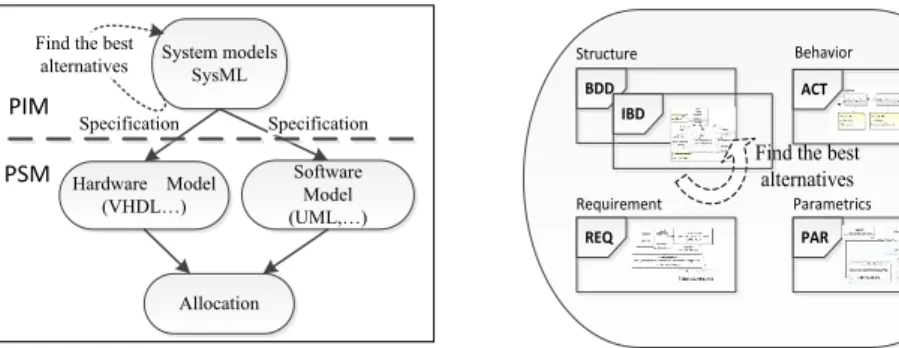
We consider architecture design in the context of systems engineering activities with MBSE, as described in [6]. The output of systems engineering activities is a system model written in SysML language (Fig. 1).

Fig. 1. Design flow with MBSE. Fig. 2. System models with SysML.

The model can be divided into a Platform Independent Model (PIM) and a Platform Specific Model (PSM). The PIM and PSM concepts come from the Model Driven Architecture standard of the Object Management Group [7]. Fig. 1 uses the model of the system to specify both hardware and software components requirements. During the PIM stage, the hardware platform is not yet selected. The designer has to consider a set of candidate platforms in order to find the best alternatives. After the specifica-tion step, the execuspecifica-tion platform is selected. In SysML, the model of the system is defined by a set of diagrams (Fig. 2). The requirement diagram (REQ) describes the

System models SysML Hardware Model (VHDL…) Software Model (UML,…) Allocation Specification Specification PIM PSM

Find the best alternatives BDD Structure Behavior REQ Requirement ACT Parametrics PAR

Find the best alternatives

requirements. The activity diagram (ACT) represents the behavior of the system. The Block Definition Diagram (BDD) and the Internal Block Diagram (IBD) describe the structure of the system. Finally the parametric diagram captures relationships among properties. An important activity of system engineering is to find the best design al-ternatives for the whole system. However the exploration space is very large, espe-cially, with current approach such as [10] that does exploration on PSM. In this paper, we focus on system model optimization issues (dashed elements in Fig. 1 and Fig. 2) because it comes first in the design activity and it will substantially restrict the design space exploration (DSE). With this approach, the DSE can be done in a stepwise manner, exploring the system model first, and then the software, hardware and alloca-tion alternatives with current DSE approaches. The system structure is also a key point for metric evaluation (i.e. cost, weight and reliability). In this context, the objec-tive for the designer using MBSE and SysML is to obtain the best trade-off system structure, in order to optimize objective functions such as cost and reliability. This multi-objective optimization problem can be described by mathematical terms:

𝑚𝑖𝑛 [𝑓1(𝒙), 𝑓2(𝒙), … 𝑓𝑛(𝒙) ] 𝑤𝑖𝑡ℎ 𝑥 ∈ 𝑆

Above, f is the objective function vector and S the set of constraints. Our approach is to suggest the best configurations to the designer, that is, to find the Pareto-optimal solutions. Pareto-optimal solutions have the lowest (or equivalently low) values for all objective functions. The set of solutions is presented to the decision-maker by the designer for the selection of optimal solutions. The methodology we propose is pre-sented by next sub-section. The requirement and structure models are adapted for the optimization, including objective function definition, variability and constraints. We assume that the system design is done using the SysML language. Also, a component repository is available including the parameters for the objective functions.

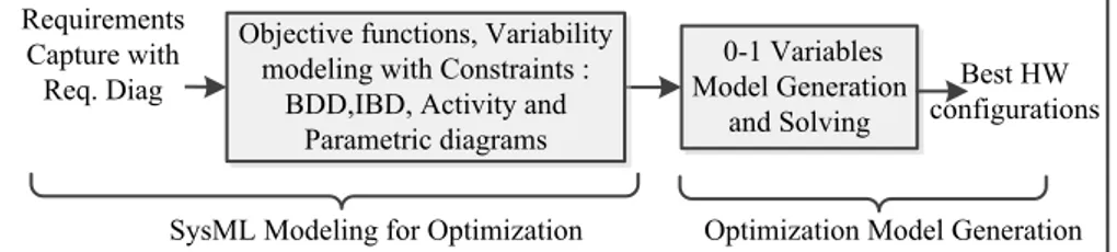
Fig. 3. Methodology overview.

Note: The SysML diagrams of this paper have been edited using the Papyrus tool from CEA [8].

2.2 Our Proposal

Fig. 3 presents the methodology we propose for optimizing system architecture, showing the activities and the produced artifacts. The first stage is the SysML model-ing for optimization (cf. section 3). In a preliminary step, the requirements are cap-tured using requirement diagrams. Architecture requirements are taken into account. This allows to express constraints and to add traceability between requirements and architecture elements. Then the SysML model is completed for optimization, by

0-1 Variables Model Generation

and Solving

SysML Modeling for Optimization Optimization Model Generation Objective functions, Variability

modeling with Constraints : BDD,IBD, Activity and

Parametric diagrams Requirements

Capture with

ing objective function definitions in parametric diagrams and by adding model varia-bility. The model variability expresses the different design alternatives the designer wants to explore. The model variability is represented by several degrees of freedom from the model, using variability variables inserted into comments. We distinguish between the instance variability variable (IVV), meaning that we may have several instances of the same component in the model, and component variability variable (CVV), meaning that a component instance may be replaced. The second stage, de-scribed in sections 4 and 5, is the optimization model generation and solving. To do this, the variability variables of the SysML model are transformed into a new set of 0-1 variables in the optimization model. By re-using the constraints from the SysML model, the problem can be resolved as a Constraint Satisfaction Problem (CSP), using a standard solver. Then the designer can select among the trade-off solutions the ones that best fit to his or her needs.

3

SysML Modeling for Optimization

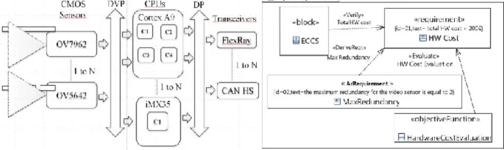
This section presents the Embedded Cognitive Safety System (Fig. 4) that serves as a running case study throughout the paper, and step-by-step discusses how to model the ECSS in SysML.

3.1 Case Study

The ECSS system can be integrated in an on-board vehicle digital system or in aero-nautics systems such as drones. Typical features for an ECSS are line detection, ob-stacle detection and distance measurement with stereoscopic view. The embedded hardware platform is composed of CMOS image sensors, processing elements and vehicle interface networks. These three components types may be redundant, for safe-ty purposes or stereoscopic processing. CMOS image sensors support auto focus en-gine and image stabilization. Image sensors are connected to processing elements through Digital Video Port (DVP), a type of parallel bus interface. Processing ele-ments are CPU supporting image processing such as Cortex A9 or iMX35. The vehi-cle interface is an embedded serial bus such as CAN High Speed or FlexRay. The vehicle interface is integrated into the ECSS system with a transceiver component, connected to the processing element with a digital port (DP) which is a parallel bus interface.

3.2 Requirements Capture

SysML provides modeling constructs to capture and represent textual requirements, and to link the requirements to other modeling elements. The requirement diagram (Fig. 5) depicts requirements, but a requirement may also appear on other diagrams to show its relationship to other modeling elements. A standard requirement includes a unique identifier and a text requirement. The “Satisfy” and “Verify” relationships relate requirements to other model elements such as blocks and test cases. In our con-text of architecture optimization, specific requirements for the architecture, so-called the “architecture requirements,” are derived from standard requirements. To clearly identify architectural requirements, a stereotype “ArRequirement” extends the stand-ard SysML requirement. On the other hand, a standstand-ard requirement is evaluated by an objective function. The objective function is a stereotype extending the standard SysML constraint block. This objective function is related to a requirement with a stereotype “evaluate” extending the basic UML-2 dependency relationship. A de-pendency is a design-time relationship between definitions. In Fig. 5, the

“MaxRe-dundancy” architecture requirement limits the sensor component redundancy to two

for cost reason, and the system cost requirement is evaluated.

3.3 MDO Context and Objective Functions Definition

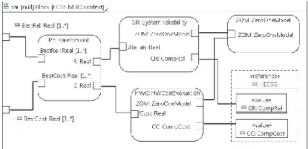
To integrate multi-domain optimization (MDO) into the system model design, we propose to define a MDO context, a type of analysis context. The MDO context is represented by a BDD diagram and a parametric diagram, both including constraint blocks. The parametric diagram captures the internal structure of a constraint block, in term of parameters and connectors between parameters. The BDD defines constraint blocks and their relationships. This BDD diagram contains a top-level constraint block, named “ECSS MDO Context” in Fig. 6. This constraint block has a reference to the block representing the system under analysis and including the variability for representing the alternatives. The MDO context diagram also contains the objective functions and the optimization model representation. The Pareto frontier, a result of the MDO context, is used to present alternatives to the designer. The MDO context can be passed to an external optimization solver, and the result can be provided back as Pareto frontier values of the MDO context. The objective function block extends the standard SysML Constraint Block and contains an optimization goal parameter (i.e. maximize or minimize). A constraint provides a description of the analytical function supporting the objective function. Other parameters specify the interaction points between the objective function and the system under analysis, and between the objective functions and the optimization model. Fig. 6 shows the MDO context defi-nition for our case study, in a BDD. The MDO context is called ECSS MDO Context, to perform a multi-objective optimization of the ECSS system. The ECSS MDO Con-text constraint block has two value vectors, /BestCost[1..*] and /BestRel [1..*], repre-senting the Pareto frontier. The ParetoFront constraint block produces these value vectors from the two objectives functions. It is intended that the equations are solved by an external optimization solver for these two vectors, so they are shown as derived.

Fig. 6. BDD diagram for ECSS MDO context Definition.

The result values obtained with an external CSP solver are presented later in section 4. As indicated by its associations, ECSS MDO context contains two constraint prop-erties, both typed by an objective function, namely HWCostEvaluation and

SystemRe-liability. A precision to the modeling of the objective function is added, with a

con-straint. The two constraints describe the equation underlying the total cost and the reliability calculation. In this case, the Python language can be used as constraint language, because it is used by the CSP solver [14]. For the SystemReliability func-tion, the system reliability R is calculated with parameters coming from the system under analysis (the components reliability) and from the Zero One Model. The ECSS MDO context also contains one reference property typed by ECSS, the system under analysis including variability. Finally, ECSS MDO contains a constraints property Zero One Model, representing the optimization model described in section 4. The Zero One Model has a parameter and a set of constraints deduced from the ECSS system (see section 4, equation 2) and from the model itself. These constraints can be expressed using the Object Constraint Language (OCL). Fig. 7 shows a parametric diagram. Its frame represents the ECSS MDO context constraint block. This diagram is similar to an internal block diagram but uses binding connectors to link constraints parameters.

3.4 System Composition and Redundancy Modeling

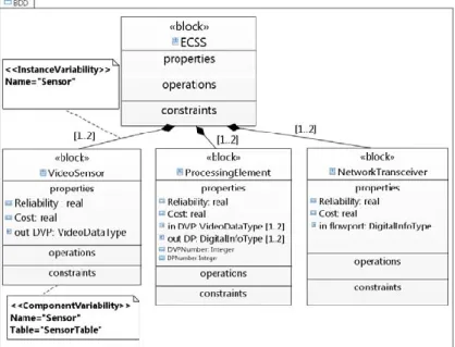
The architecture modeling represents the set of hardware resources available for the execution of the application. The hardware system is made up of several components and described by a block definition diagram (see Fig. 8). In our optimization problem, the composition is known, but the redundancy level of each component is not. The redundancy level is the first degree of freedom for the optimization problem. At this step, we specify instance variability variables (IVV) in comments. Each IVV is relat-ed to a composition association, between the top-level component and the low-level component. The ECSS system in Fig. 8 contains one or two sensors, processing ele-ments and networks. Three IVVs are respectively related to the sensor, the CPU and the Transceiver composition.

Fig. 8. BDD for HW composition.

The hardware components selection is the second degree of freedom for the optimiza-tion process. For this second degree of freedom, a Component Variability Variable (CVV) is inserted in the model as a comment. A CVV indicates that the component instance can be replaced by another hardware component specification. The hardware component specification is provided by the designer, and belongs to a component repository. The repository includes a set of tables. Each table is associated with one component of the block definition diagram. In our example, we define three tables and three CVV, respectively associated with the sensor, the processing element and the network block. Each table contains the list of available components, with their cost and reliability (See Table 2). The user, in addition to the SysML model, provides these tables.

3.5 Component Interface Modeling

Component interface modeling is useful for the optimization problem, because new constraints arise during this stage. These constraints will be added to the computa-tional model for the problem solving. The Internal Block Diagram in SysML captures the internal structure of a block in terms of properties and connectors between proper-ties. If we consider the IBD depicted by Fig. 10, we have one or two sensors with one output DVP port connected to one or two processing elements for video data trans-mission. At this step, the goal is to retain the valid configurations with a constraint used by the optimization process. In our case and for the digital video port (DVP), the sum of input ports for processing elements shall be greater than or equal to the sum of output port for video sensors. This constraint may be expressed in OCL and attached to the VideoData connection.

4

Problem Statement

Previous section has shown how the SysML model could be prepared for optimiza-tion. But a mathematical representation is required to perform the optimization with suitable algorithms. In this section we propose a representation and show how to ob-tain it from the SysML model. This representation is based on zero-one variables, and can be solved as a constraint satisfaction problem. Optimization models have been developed to select software or hardware components and redundancy levels. The system (see Fig. 9) consists of independent subsystem Si. Si is associated to a given block with instance variability (the VideoSensors aggregation in Fig. 9). Subsystem Si is composed of components selected in a repository of components Ci. Cij represents the component number j in the repository Ci. Each selected component has a position k in the final subsystem Si, after the problem resolution. Fig. 9 shows there exists two possible positions for a selected component in the final subsystem Si.

Fig. 9. from BDD to problem formulation. Fig. 10. From IBD to connection constraints

S

S

S

IBD

We define the following sets and parameters:

 Si the set of components with position k. Ci the set of components available in the

component repository

 cij the cost of component Cij and θi an interconnection cost for any component

 rij the reliability of component Cij

 eij and sij the input and output port numbers of component Cij. For sensors (the first

block) we have no input port and one output port, so we have : e1j=0 and s1j=1

These sets and parameters are deduced from the SysML model, as it is shown in Ta-ble 1.

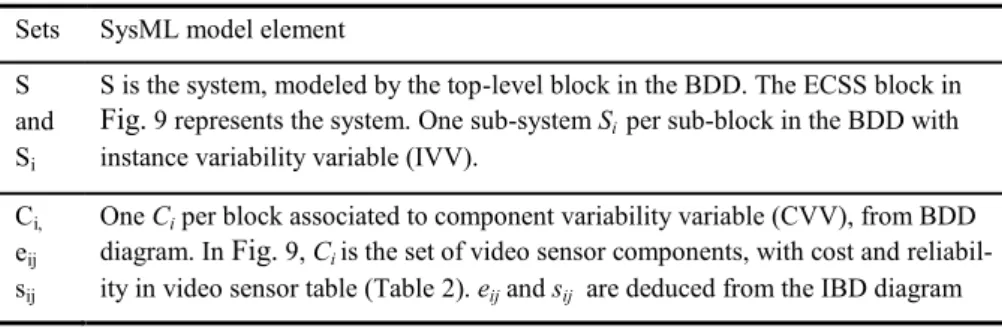
Table 1. Association between SysML model elements and optimization model.

Sets SysML model element S

and Si

S is the system, modeled by the top-level block in the BDD. The ECSS block in

Fig. 9 represents the system. One sub-system Si per sub-block in the BDD with instance variability variable (IVV).

Ci, eij sij

One Ci per block associated to component variability variable (CVV), from BDD diagram. In Fig. 9, Ci is the set of video sensor components, with cost and reliabil-ity in video sensor table (Table 2). eij and sij are deduced from the IBD diagram

In Fig. 9, the range of k is given by the SysML aggregation multiplicity in the BDD, the range of i by the system composition in the BDD and the range of j by the component table size. The following zero-one programming formulation of this prob-lem defines decision variables:

∀𝑖 ∈ 𝑆, 𝑗 ∈ 𝐶𝑖, 𝑘 ∈ 𝑆𝑖 𝑎𝑖𝑗𝑘= {0 𝑖𝑓 𝑐𝑜𝑚𝑝𝑜𝑛𝑒𝑛𝑡 𝐶_{1 𝑜𝑡ℎ𝑒𝑟𝑤𝑖𝑠𝑒} 𝑖𝑗 𝑖𝑠 𝑢𝑠𝑒𝑑 𝑖𝑛 𝑝𝑜𝑠𝑖𝑡𝑖𝑜𝑛 𝑘 𝑜𝑓 𝑆𝑖 (1)

Seen as constraints applied to the system, the first set of constraints comes from the decision variable definition.

At any position of the final subsystem Si we can have only one component in position k :

∀𝑖, 𝑗 ∑ 𝑎𝑖𝑗𝑘≤ 1 (2) 𝑘

Other constraints can be expressed such as exclusion between components. When a CPU component is not compatible with a particular transceiver, this can be expressed as a constraint, such as a sum lower than one. In the same way, a sum comparison is used to express a component dependency. Connection information is given by the IBD diagram (see Fig. 10). First, the place of each Si in the component flow is given. Then the connection constraints are provided. At each interface we have constraints between the total input port number and the total output port number. In Fig.10, for

VideoData connection, the sensors and CPUs satisfy the following connection

∑ 𝑎1𝑗𝑘𝑠1𝑗≤ ∑ 𝑎2𝑗𝑘𝑒2𝑗 𝑗,𝑘 𝑗,𝑘

(3)

For DigitalData connection, each transceiver input is connected to one CPU, and each CPU has at least one connected output:

∑ 𝑎3𝑗𝑘𝑒3𝑗≤ ∑ 𝑎2𝑗𝑘𝑠2𝑗 𝑗,𝑘 𝑗,𝑘 and ∑ 𝑎2𝑗𝑘𝑠2𝑗≤ ∑ 𝑎3𝑗𝑘𝑒3𝑗 𝑗,𝑘 𝑗,𝑘 (4) The objective functions are included in the parametric diagram. In our example, the goal is to minimize the cost and to maximize reliability. The total system cost includ-ing interconnection cost is given by equation (5). The system reliability to be maxim-ized, using serial-parallel interconnection model, can be calculated by equation (6).

min 𝐶 = ∑ 𝑐𝑖𝑗[𝑎𝑖𝑗𝑘+ 𝑒𝑥𝑝 (𝜃𝑖∑ 𝑎𝑖𝑗𝑘 𝑘 )] 𝑖,𝑗,𝑘 (5) max 𝑅 = ∏ [1 − ∏[1 − 𝑎𝑖𝑗𝑘𝑟𝑖𝑗] 𝑗,𝑘 ] 𝑖 (6)

5

Model Transformation

In this section, CSP problems are presented, and a formalization for the system under analysis (SuA) is proposed.

5.1 CSP Problem

The problem defined in sub-section 4 including variables and constraints can be seen as a constraint satisfaction problem (CSP). A CSP, as defined in [13] consists of a set of n variables 𝑋 = {𝑥1, 𝑥2, … 𝑥𝑛}, a set of n domains 𝐷 = {𝐷1, 𝐷2, … 𝐷𝑛} 𝑤𝑖𝑡ℎ 𝑥𝑖∈ 𝐷𝑖, a set of constraints and a set of objective functions F = {f1, f2, … fi}. A function fi is an objective function which maps every solution to a numerical value.

Researchers in artificial intelligence usually adopt CSP to solve problems such as scheduling or decision problems. CSP problems are combinatorial by nature. They are NP-complete or NP-hard (RM Karp, [17]). An efficient algorithm (i.e with polynomi-al time for polynomi-all inputs) does not exist, but some heuristics produce good approximate solutions. A feasible solution for the problem consists in an assignment of values from its domain to every variable, in such a way that each constraint is satisfied. When a feasible solution exists, we may want to find just one solution, all solutions or an optimal solution. In our case we want to find optimal solutions. An optimal solu-tion is given by the objective funcsolu-tions defined in the SysML model. The selected approach in this paper consists in finding all solutions of the CSP problem and then to evaluate the different solutions with objective functions, to determine the optimal solutions. Algorithms for solving CSP use to systematically search through the possi-ble assignments of values to find a solution. SC Brailsford et al. [13] show that a sim-ple algorithm is the backtracking algorithm, and others are forward checking and the MAC algorithm. These algorithms use a search tree, as it would be done in a branch and bound algorithm. In the backtracking algorithm, the current variable is assigned

to a value from its domain. This assignment is checked against the current partial solution. If any of the constraints is violated, another value for the current variable is chosen. If all the values have been tried, the algorithm backtracks to the previous variable and assigns it with another value. A CSP solver typically uses a problem description file to define the problem. This file is written in high level programming language such as Python and contains several sections. The first one is the variables definition, including the variable names, the data types and variables bounds. Depend-ing on the solver, data types can be integer, Boolean, choice or real. The second sec-tion is the constraints secsec-tion, with relasec-tionships of equality or inequality between variables. The problem to solve is created with a particular command, and the previ-ous variables and constraints are added to the problem. Lastly, a resolution command is used to invoke the solver algorithm for the problem solving.

5.2 Creation of CSP Variables

The appropriate variables are created in the CSP description file, from the SuA in-cluding variability. When a combination between component and instance variability is found, as it is described in Fig. 9, we create a two dimensional array of Boolean variables, corresponding to the 𝑎𝑖𝑗𝑘, ∈ {0,1} coefficients described in equation (1).

We obtain the following lines of code in the first section of the CSP problem de-scription file. These lines create a two dimensional array of Boolean variables 𝑎𝑖𝑗 for the problem, corresponding to the sensors variability. The variability is a combination of single or dual redundancy, and a list of two sensors:

problem.addVariables(["a"+str(i)+str(j) for j in range(1,3) for i in range(1,3)], [0,1])

5.3 Constraints and CSP Resolution

The second section of the CSP problem description file includes the constraints coming from the SysML model and from the representation of variables. For the rep-resentation of variables, when a combination between component and instance varia-bility is found, the constraint expressed by equation (2) is inserted in the problem description file. The following lines of code correspond to the sensors representation in the case study:

problem.addConstraint(lambda a11,a12, : a11+a12 <= 1, ("a11","a12"))

problem.addConstraint(lambda a21,a22, : a21+a22 <= 1, ("a21","a22"))

The other constraints come from constraint blocks in the SysML model. The Internal Block Diagram in Fig. 10 provides constraints between the total input port number and the total output port number, for the sensors, the CPUs and the transceiver. These constraints are expressed by equations (3), (4), given in section 4. In equation (3), one

sensor shall be connected to one CPU having one or two inputs. This corresponds to the following lines of code in the CSP problem description file of our case study: problem.addConstraint(lambda

a11,a12,a21,a22,b11,b12,b21,b22 : 2*b11+b12+2*b21+b22 >= a11+a12+a21+a22,

["a11","a12","a21","a22","b11","b12","b21","b22"])

After the variable definition and the constraints instantiation, the CSP problem can be solved and the solutions are sorted with the following lines:

solutions = sorted(sorted(x.items()) for x in prob-lem.getSolutions())

Regarding the case study, as a first experiment, we obtain a CSP problem with Boole-an variables, 𝑎𝑖𝑗, 𝑏𝑖𝑗, 𝑐𝑖𝑗 𝑤𝑖𝑡ℎ 𝑖, 𝑗 ∈ {1,2} for the sensors, the CPUs and the trans-ceivers. The resolution of this constraint problem provides seventy-four CSP solu-tions, after the filtering of equivalent configurations due to the Boolean representa-tion.

5.4 Evaluation of the CSP solutions

After obtaining the CSP solutions, each solution can be evaluated with the objective functions. An objective function is expressed with an algorithm included in a con-straint block of the optimization context. In Fig. 6, the “SystemReliability” and the “HWCostEvaluation” constraint blocks contain Python code of the objective functions given by equations (5) and (6).

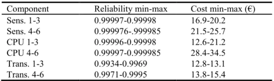
Table 2. Component repository extract.

Component Reliability min-max Cost min-max (€)

Sens. 1-3 0.99997-0.99998 16.9-20.2 Sens. 4-6 0.999976-.999985 21.5-25.7 CPU 1-3 0.99996-0.99998 12.6-21.2 CPU 4-6 0.99997-0.999985 28.4-34.5 Trans. 1-3 0.9934-0.9969 12.8-13.1 Trans. 4-6 0.9971-0.9995 13.8-15.4

The input parameters for the algorithms are the 𝑎𝑖𝑗, 𝑏𝑖𝑗, 𝑐𝑖𝑗 coefficients and the cost and reliability of each component in the repository (see Table 2). The 𝑎𝑖𝑗, 𝑏𝑖𝑗, 𝑏𝑖𝑗 ∈ {0,1} coefficients are defined in equation (1) and correspond to the decision varia-bles. By applying the algorithm of the objective functions (Cost and reliability) to each solution of the CSP problem, we get results in the following form:

Solution 39

a11 a12 = 01 b11 b12 = 01 c11 c12 = 01 a21 a22 = 01 b21 b22 = 01 c21 c22 = 10 Fail. R.=0.00001484 Cost=95

This result means that the solution #39 to the CSP problem has a hardware cost of €95 and a failure rate of 14.8 failures per million. This solution is obtained by using two identical sensors of type 2, two identical CPUs of type 2, and two transceivers of type 1 and 2.

5.5 Pareto frontier

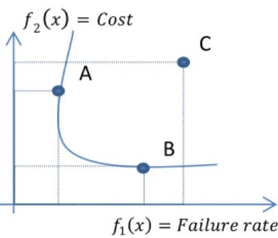
From the set of solutions obtained in previous section, it is possible to extract the Pareto frontier. Each solution represents an alternative for the system design. General-ly speaking, the Pareto frontier consists of all alternatives that are not dominated by another one. In Fig. 11, the A alternative dominates C because A is both cheaper and more reliable than C. But A and B do not dominate each other.

Fig. 11. Pareto frontier

For a minimization problem, an alternative named A dominates another one named C if and only if:

{∀𝑖 ∈ {1. . 𝑛} 𝑓_{∃𝑖 ∈ {1. . 𝑛} 𝑓}𝑖(𝒂) ≤ 𝑓𝑖(𝒄) 𝑖(𝒂) < 𝑓𝑖(𝒄)

𝑤𝑖𝑡ℎ 𝒇(𝒙) = (𝑓1(𝒙), 𝑓2(𝒙), … 𝑓𝑛(𝒙)) is an array of n objective functions. 𝒙 is the array of decision variables. In the context of our case study, we have:

𝒙 = {𝑎11, 𝑎12, . . , 𝑏11, 𝑏12, . . , 𝑐11, 𝑐12, . . } with 𝑎𝑖𝑗, 𝑏𝑖𝑗, 𝑐𝑖𝑗 ∈ {0,1} defined in equation (1), 𝑓1(𝑥) is the failure rate and 𝑓2(𝑥) is the system cost. After solving the CSP prob-lem in previous section, we obtained an array 𝑺 of n solutions with a cost and failure rate estimation. In order to obtain the Pareto frontier 𝑃, we apply Algorithm 1. In line 2, the solutions are sorted according to their increasing cost (primary sort key) and according to their increasing failure rate (secondary sort key). We obtain a second 𝑺′ array of solutions. In line 4, the cheapest solution (first solution of 𝑺′) is added to the Pareto Frontier. Then we skip the successive alternatives until we find one with a lower or equal failure rate (line 7 and 8). This alternative is added to the Pareto fron-tier and the search is restarted from this alternative.

With this algorithm, when several alternatives have the same cost and the same failure rate, they are all added to the Pareto frontier, if they are not dominated by an-other solution. 𝑓1(𝑥) = 𝐹𝑎𝑖𝑙𝑢𝑟𝑒 𝑟𝑎𝑡𝑒

A

B

C

(

)

Algorithm 1: Pareto frontier extraction from a solution set

1. 𝑃 ← ∅ , 𝑖𝑛𝑑𝑒𝑥 ← 1, 𝐼𝑡𝑒𝑚𝐹𝑜𝑢𝑛𝑑 ← 𝑇𝑟𝑢𝑒

2. Sort 𝑆 array in order of increasing cost and increasing failure rate, we obtain 𝑆′₌ (𝑆1, 𝑆2, … 𝑆𝑛) 3. 𝑾𝒉𝒊𝒍𝒆(𝐼𝑡𝑒𝑚𝐹𝑜𝑢𝑛𝑑 = 𝑇𝑟𝑢𝑒) 4. 𝑨𝒅𝒅 𝑆′𝑖𝑛𝑑𝑒𝑥 𝒕𝒐 𝑃 5. 𝐼𝑡𝑒𝑚𝐹𝑜𝑢𝑛𝑑 ← 𝐹𝑎𝑙𝑠𝑒 6. 𝑭𝒐𝒓(𝑗 = 𝑖𝑛𝑑𝑒𝑥 + 1 𝑡𝑜 𝑛) 7. 𝒊𝒇(𝐹𝑎𝑖𝑙𝑢𝑟𝑒𝑅(𝑆′ 𝑗) ≤ 𝐹𝑎𝑖𝑙𝑢𝑟𝑒𝑅(𝑆′𝑖𝑛𝑑𝑒𝑥)) 8. 𝑖𝑛𝑑𝑒𝑥 ← 𝑗, 𝐼𝑡𝑒𝑚𝐹𝑜𝑢𝑛𝑑 ← 𝑇𝑟𝑢𝑒 9. 𝑬𝒏𝒅𝑭𝒐𝒓 10. 𝑬𝒏𝒅𝑾𝒉𝒊𝒍𝒆 11. 𝑹𝒆𝒕𝒖𝒓𝒏 𝑃 5.6 Results

We consider the case study with a maximum redundancy of two and four connection constraints between sensors, processing elements and network transceivers. A reposi-tory of 18 components is specified in Table 2. We obtain a 36-decision variables problem to be solved. With the CSP solver using a backtracking algorithm imple-mented in Python, and a posteriori objective function evaluation, we obtain 13,500 solutions in 36 minutes of computation time (Fig. 12). The X-axis displays the Failure rate (1-Rs) instead of reliability Rs. The figure is obtained with a MATLAB [16] im-plementation of algorithm 1 running on an Intel i5 3GHz machine with 4 GB RAM. Each point figures a solution to the CSP problem obtained with the Python labix solv-er [14]. The solid line figures the Pareto frontisolv-er.

Fig. 12. Pareto frontier with CSP Solver

For a maximum cost of €90 and a failure rate < 0.00002, table 3 presents the three best trade-off configurations selected by the user.

Table 3. Three best trade-off configurations

Solution # Sensors CPUs Transceivers Cost (€) FR (10-5)

1 S1+S1 CPU1 T4+T1 73 1.48

2 S1+S3 CPU1 T1+T1 75.3 1.22

3 S1+S3 CPU1+CPU1 T1+T1 87.9 1.02

6

Related work

In recent literature, there are approaches such as [15], [4] or [5] on the architecture optimization at the system level with SysML. In [15], the authors have demonstrated the adaptability of SysML by extending the language to provide integration with mathematical solver for optimization. However this approach lacks support of multi-criteria optimization that would help designers to perform design space exploration and trade-off analysis. The approach proposed by P. Van Huong [4] and Spyropoulos [5] allows the user to perform multiple analyses in the same environment. These ap-proaches are adapted to the component parameters optimization such as CPU fre-quency or memory size, not to the architecture composition and redundancy problem we want to address. In [9] an optimization technique is proposed for a microwave module design, with combination of alternatives for part modules, but without redun-dancy constraint. In the Design Space Exploration (DSE) approach ([10]), the prob-lem to solve is related to the hardware/software partitioning and the mapping of appli-cation onto hardware elements. Our approach comes earlier in the design flow and is complementary, providing a limitation of the design space exploration. The redun-dancy allocation problem (RAP, [11], [12]) deals with component selection, for cost and reliability optimization at system level. In these approaches (DSE, RAP), the problem is formalized as an optimization problem, and not with the MBSE approach. Similarly, in the RAP formulation the connection topology is fixed as a serial-parallel model.

7

Conclusions and Future Work

The paper presents a methodology for multi-objective optimization of system ar-chitecture. Starting from a SysML model, we add information concerning objective functions, variability and architecture constraints. The redundancy level and the com-ponent alternatives are tagged with variables that describe variability. Then the SysML model can be further exploited to generate a mathematical representation, based on integer variables, linear constraints and objective functions. The problem can be solved using a CSP solver. Finally, the ECSS case study shows that there ex-ists three best configurations, minimizing cost and maximizing reliability, from a repository of 18 components. Ongoing work includes the integration of two steps in the methodology, the deployment and the system configuration. The deployment is the allocation of software components onto hardware components. The configuration is the determination of the best values for model attributes such as ECSS position in

the vehicle. For the deployment and configuration, the variability concept shall be extended. In particular, for the system configuration, the variables can be either dis-crete or continuous. That is why in addition to instance and component variability, the value variability, relative to component attributes, will be integrated too. The CSP problem generation shall be adapted too, to cope with the resolution of these mixed problems, including discrete and continuous variables.

8

References

1. OMG Systems Modeling Language (OMG SysML™), V1.3, http://www.omg.org/spec/SysML/1.3/PDF

2. TOPCASED, The Open source Toolkit for critical systems; http://www.topcased.org/

3. TTool, The TURTLE Toolkit, http://labsoc.comelec.telecom-paristech.fr/ttool.

4. Van Huong, P., & Binh: Embedded System Architecture Design and Optimization at the Model Level., IJCCE, vol. 1, no. 4, pp. 345-349. IAP, San Bernardino (2012)

5. Spyropoulos, D., & Baras: Extending Design Capabilities of SysML with Trade-off Anal-ysis: Electrical Microgrid Case Study. Procedia Computer Science, 16, 108-117. Elsevier, Amsterdam (2013)

6. Friedenthal, S., Moore, A., & Steiner: A practical guide to SysML; The MK/OMG Press,San Francisco (2009)

7. MDA, the Model Driven Architecture; http://www.omg.org/mda/ 8. Papyrus tool from CEA, http://www.eclipse.org/papyrus/

9. Meyer, J., Ball, M., Baras, J., Chowdhury, A., Lin, E., Nau, D., ... & Trichur, V.: Process Planning in Microwave Module Production. Artificial Intelligence and Manufacturing: State of the Art and State of Practice. (1998)

10. Apvrille, L.: TTool for DIPLODOCUS: an environment for design space exploration. In Proceedings of the 8th international conference on New technologies in distributed sys-tems (p. 28). ACM. (2008)

11. Coit, D. W., & Smith, A. E: Optimization approaches to the redundancy allocation prob-lem for series-parallel systems. In Fourth Industrial Engineering Research Conference Pro-ceedings (pp. 342-349). Citeseer, (1995)

12. Limbourg, P., & Kochs, H. D.:. Multi-objective optimization of generalized reliability de-sign problems using feature models—A concept for early dede-sign stages. Reliability Engi-neering & System Safety, 93(6), 815-828. Elsevier, Amsterdam (2008)

13. Brailsford, S. C., Potts, C. N., & Smith, 1999. Constraint satisfaction problems: Algo-rithms and applications. European Journal of Operational Research, 119(3), 557-581. Elsevier, Amsterdam (2009)

14. Niemeyer G, python-constraint, http://labix.org/doc/constraint/

15. Schamai, W., Fritzson, P., Paredis, C., & Pop, A. : Towards unified system modeling and simulation with ModelicaML: modeling of executable behavior using graphical notations. In Proceedings 7th Modelica Conference, Como (2009)

16. Mathews, J. H., & Fink, K. D.:. Numerical methods using MATLAB (Vol. 31). Prentice hall Upper Saddle River, NJ (1999).

17. Karp, Richard .M., : Reducibility among combinatorial problems. In: Miller, R.E., pp. 85–103. Springer US (1972)