Any correspondence concerning this service should be sent to the repository
administrator:
[email protected]
O
pen
A
rchive
T
OULOUSE
A
rchive
O
uverte (
OATAO
)
OATAO is an open access repository that collects the work of Toulouse researchers and
makes it freely available over the web where possible.
This is an author-deposited version published in:
http://oatao.univ-toulouse.fr/
Eprints ID: 16572
To cite this version:
Denieul, Yann and Alazard, Daniel and Bordeneuve-Guibé, Joël and
Toussaint, Clément and Taquin, Gilles Interactions of Aircraft Design and Control:
Actuators Sizing and Optimization for an Unstable Blended Wing-Body. (2015) In: AIAA
Atmospheric Flight Mechanics Conference, 22 June 2015 - 26 June 2015 (Dallas, Texas,
United States).
Interactions of Aircraft Design and Control: Actuators
Sizing and Optimization for an Unstable Blended
Wing-Body
Yann Denieul
∗Daniel Alazard
†Joel Bordeneuve
†University of Toulouse, ISAE-SUPAERO, 10, Av. Edouard Belin, 31055 Toulouse FRANCE
Clement Toussaint
‡ONERA, 2, Av. Edouard Belin, 31055 Toulouse FRANCE
Gilles Taquin
§Airbus Operations SAS, 316 route de Bayonne, 31060 Toulouse FRANCE
In this paper the problem of integrated design and control for a civil blended wing-body aircraft is addressed. Indeed this configuration faces remarkable challenges related to handling qualities: namely the aircraft configuration in this study features a strong lon-gitudinal instability for some specific flight points. Moreover it may lack control efficiency despite large and redundant movables. Stabilizing such a configuration may then lead to high control surfaces rates, meaning significant energy penalty and installation mass for flight control actuators, as well as challenges for actuators space allocation. Those penal-ties should therefore be taken into account early in the conceptual design phase, instead of being checked afterwards. Our approach consists in simultaneously designing a stabilizing controller and actuators dynamic characteristics, namely their bandwidth, for a given air-craft configuration. Our method relies on latest developments on nonsmooth optimization techniques for robust control design. For any aircraft configuration, guaranteed stability performance, as well as optimized control surfaces allocation with respect to their relative
efficiency and inertia, are obtained. From these results, a segregation among trim and
maneuver control surfaces is obtained, with guarantee that the later ones are able to cope with aircraft instability. Then it is checked that remaining trim control surfaces are suffi-cient for equilibrating the aircraft in any flight condition. This approach allows for a fast prototyping of control surfaces and actuators for unstable configurations. Different control surfaces layouts are evaluated in order to show the flexibility of the method.
Nomenclature
α Angle of attackCD Drag coefficient
Cm Pitching moment
Cm0 Zero-lift pitching moment
Cmq Pitching moment pitch rate gradient
CL Lift coefficient
CLq Lift coefficient pitch rate gradient δm Control surface deflection
∗PhD Student, University of Toulouse, ISAE-SUPAERO, 10, Av. Edouard Belin, 31055 Toulouse FRANCE. †Professor, University of Toulouse, ISAE-SUPAERO, 10, Av. Edouard Belin, 31055 Toulouse FRANCE. ‡Research Engineer, ONERA, 2, Av. Edouard Belin, 31055 Toulouse FRANCE.
γ Flight path angle ρ Volumetric mass θ Pitch attitude ω Actuator bandwidth
B Aircraft inertia around ya axis
AVL Athena Vortex Lattice BWB Blended Wing-Body CG Center of Gravity CoP Center of Pressure
EMA Electro-Mechanical Actuator FCS Flight Control System GW Gross Weight
HM Hinge Moment
HWB Hybrid Wing-Body i i-th control surface
K Compensator
l Reference length LQ Linear Quadratic
LMI Linear Matrix Inequalities LoD Lift-over Drag ratio m Aircraft mass
MTOW Maximum Taike-Off Weight MDO Multi-Disciplinary Optimization OWE Operating Weight Empty ncontrols number of control surfaces
RSS Relaxed Static Stability S Reference area
SAS Stability Augmentation System S&C Stability and Control
u Command
V Aerodynamic speed
W&CG Weight and Center of Gravity
I.
Introduction
Among other disruptive aircraft configurations, the Flying Wing (also known in litterature as Blended Wing-Body (BWB)1 or more recently Hybrid Wing-Body2) has been identified for years as a potential
candidate for the future of civil aviation.3 Most studies in this field focused either on the overall aircraft
design problem, optimizing the aircraft with respect to ”traditional” disciplines in the conceptual design phase, such as aerodynamics, propulsion, weights and performance1,4 or on stability and control related
challenges for a given configuration.5 However this sequential approach, while valid for traditional aircraft
configurations, appears as too restrictive for the BWB case. Indeed its unusual characteristics, such as a strong longitudinal instability, do not allow treating the handling qualities issues without considering active stabilisation in the early design phase6.7 At Airbus previous research topics were focusing on plan form
optimization for performance objectives on the one hand, and handling qualities resolution8 on the other
hand. This meant checking regulation and in-house criteria for maneuvers, in flight and on ground equilibria. One of the conclusions of these studies was the need for active stabilisation. It was also concluded that the active stabilisation may induce high deflection rates on control surfaces; this is even more problematic as these surfaces may be significantly larger than usual movables. They may also lack pitch efficiency. As a result a major mass and energy penalty would result from flight control actuators required to stabilize the aircraft. What we propose to perform here is a synthesis of these couplings between aircraft design and control, as well as setting a process capable of sizing and optimizing the flight control actuators in a preliminary way for dynamic stability criteria. This paper is organized as follows: in section II the general problem of stabilizing an aircraft with redundant actuators is adressed, the aerodynamic model and the
different control surfaces layouts are presented. Then section III presents the problem of integrated design and control, and the specific H2/H∞ formulation used in this paper in order to simultaneously optimize
the controller and the actuators bandwidth. The objective is to meet constraints on handling qualities requirements while minimizing the ”cost” of actuators. Finally section IV discusses the results obtained for different control surfaces layouts in terms of achievable actuators bandwidth and remaining trim capability.
II.
Problem Setup
II.A. Design Challenges associated to the Control of an Unstable Configuration
From a handling qualities point of view, an aircraft is said statically stable if its center of gravity (CG)9
is located forwards its aerodynamic centera. The aerodynamic center of an aircraft is mainly driven by its
lifting surfaces characteristics, ie wing location with respect to the fuselage, airfoils and twist. Whereas static stability, or at least neutral stability, used to be a design constraint at preliminary design stage, recent aircraft designs tend towards instability. From a conceptual design point of view, Relaxed Static Stability (RSS) may be seeked for different reasons:
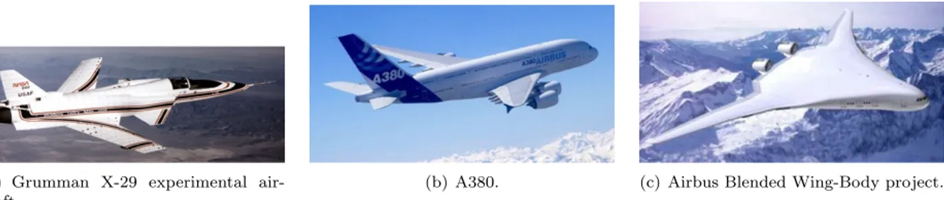
• High levels of instability enable excellent maneuverability properties for fighter aircraft. For instance the X-36 tailless demonstrator10or the Grumman X-29 forward-swept wing experimental aircraft (see
figure 1(a)), are both designed with negative static stability margins (35%l for the X-2911); as a result
any perturbation from an initial longitudinal equilibrium makes the aircraft dynamically depart. If this motion is adequately controlled, superior longitudinal maneuverability is obtained.
• For civil commercial aircraft, RSS may be a desirable feature for cruise performance optimization. In-deed a conventional statically stable tail-aft configuration requires a downlift force on the aft horizontal stabilizer in order to trim the aircraft in cruise. This results in higher lift coefficient on the main wing, therefore in higher induced and wave drag . Reducing the static margin by shifting the CG backwards and diminishing the horizontal tailplane size is therefore beneficial from a lift-over-drag ratio (LoD) point of viewb: the induced drag and wetted area are decreased (see for instance the A380 figure 1(b)).
Of course levels of instability for such configurations are not in the same order of magnitude as for super-maneuverable fighter aircraft.
• However for some configurations instability is no more a design requirement, but a consequence of an overall layout. On the BWB studied in this paper (see figure 1(c)), planform and airfoil design results of optimisation of the LoD with constraints on the zero-lift pitching moment Cm0 to ensure a
feasible take-off rotation despite the nose-down pitching moment of the high-mounted engines.12 The
aerodynamic center then comes as an output of the optimization process. The specific lift distribution of the BWB, featuring a large lifting centerbody, implies generally a large lift produced at the forward part of the aircraft. This tends to move the aerodynamic center forward. On the contrary fuel located in the wing box tends to move the CG backwards, resulting in a negative static margin and a strong instability for some flight points (see on figure 2 the relative position of the CG and aerodynamic center for different masses and speeds). It should be noted however that instability is not inherent to the BWB configuration. In the work of Lyu and Martins for instance4,13an optimization is performed on
the planform and profiles of a BWB with constraints on cruise trim and minimum static margin. The resulting geometry is optimal from a LoD point of view within the constraints — therefore the optimal LoD is slightly decreased with respect to optimal LoD without stability constraint—, and remains stable and equilibrated.
A question then arises: for a given configuration, are we able to adequately control its unstable modes, and at which expense on the flight control system (FCS) cost and complexity? Indeed it was shown in previous aFrom a dynamic point of view, the appropriate point to be considered for stability is the maneuver point. If the CG is at
the maneuver point position, then the short period mode is at limit of stability. This point lies backwards the aerodynamic center, due to Cmq and CLq damping effects. On a conventional tail-aft configuration, Cmq effect can be significant due to
tail lever arm. On the contrary on a BWB Cmqeffect is very small, meaning that aerodynamic center and maneuver point are
nearly equivalent.
bMore precisely trim drag is minimal for the CG located at a so-called Center of Pressure — CoP —. For a CG located
at the CoP no pitching moment is needed to balance the aircraft. The aircraft CoP lies backwards the aerodynamic center: therefore going towards this point tends to increase the aircraft instability.
(a) Grumman X-29 experimental air-craft.
(b) A380. (c) Airbus Blended Wing-Body project.
Figure 1. Illustration on unstable aircraft configuration for different design purposes.
studies that despite constant advances in the field of Control, fundamental physical limitations remain when controlling an unstable plant. A seminal lecture by Stein14 emphasises the fact that a controlled
unstable mode remains only locally stable, and turns unstable again when reaching non-linearities such as actuators saturations and rate limits. Whatever the control method used, physical limitations such as actuators bandwidth and rate limits, sensors and processors sampling rates, mechanical structure modes prevent from controlling high frequency unstable modes. A consequence of this is illustrated in a paper by Rogers and Collins11 about X-29 control synthesis. Two control methods, namely H
2 and H∞ design are
compared. From a theoretical point of view the H∞design exhibits superior performance, however actuators
limitations are largely exceeded. When taking into account those limitations into the control design, both methods perform equally, but neither is able to meet the requirements.
The aim of this study is to determine the required actuators dynamics that stabilize our configuration with appropriate performance, by taking advantage of the redundant actuators on the whole trailing edge, as can be seen on figure 3(a). Actuators sizing for BWB large control surfaces with possibly high deflection rates has been identified for years as a challenging task.15 Quoting a seminal paper on BWB configuration by
Liebeck,3”If the BWB is designed with negative static margin (unstable), it will require active flight control
with a high bandwidth, and the control system power required may be prohibitive”. Indeed as stated by Garmendia et al.,16 secondary power for FCS P
F CS may be evaluated in a preliminary way by the equation
1: PF CS= ncontrols X i=1 HMimax. ˙θmaxi (1) where HMmax
i and ˙θimaxare the maximum hinge moment and maximum deflection rate of the i-th control
surface respectively, and ncontrols is the number of control surfaces.
• On the one hand, from Roman et al.1 we know that hinge moments are related to the scale of a
control surface through a ”square-cube law”: control surface area increases as the square of the scale λ2, whereas hinge moment increases with the cube of this scale λ3. Large BWB control surfaces lead to high hinge moments requirements. However hinge moments computation is out of scope of this study. • On the other hand, deflection rate is a direct consequence of a stability augmentation system (SAS) for an unstable configuration. It can be demonstrated that under the assumptions of a linear dynamic model with static state-feedback compensator K and actuator modeled by a first-order transfer function with bandwidth ω (for notations please refer to figure 7):
yact
uact
= ω
ω + s (2)
The maximal deflection rate ˙θmax for an initial perturbation X
0 on the aircraft states — e.g. a
perturbation on the angle of attack — is obtained at the initial time and is equal to: ˙θmax= ˙θ
0= ωK(X0− Xeq) (3)
This means that deflection rates are both a function of the actuators dynamics and the control law synthesis.
The aim of this study is then to perform a combined synthesis of control laws and actuators bandwidth sizing, in order to limit deflection rates induced by the SAS. Keeping in mind previous remarks on hinge moments, deflection rates should moreover be more limited for larger control surfaces.
Figure 2. Weight & CG diagram of the studied BWB, and aerodynamic center in low speed (blue) and high speed (red) in percentage of Mean Aerodynamic Chord (MAC).
II.B. The Blended Wing-Body Configuration
In this section the aerodynamic model as well as the three evaluated control surfaces layouts are described. II.B.1. Aerodynamic Model
The flight dynamics model used in this study comprises only longitudinal equations written in the aerody-namic reference system Ra(xa, ya, za):
m ˙V = −1 2ρV 2SC D− mg sin γ + F (4) −mV ˙γ = −12ρV2SCL+ mg cos γ (5) B ˙q = 1 2ρV 2SlC m (6) ˙θ = q (7) θ = α + γ (8) where:
• concerning aircraft parameters, m and B denote the aircraft mass and inertia around the ya axis
respectively, S and l are reference surface and length, corresponding to the wing aera and mean aerodynamic chord respectively.
• angles are classically defined as follows: γ, α and θ denote the flight path angle, angle of attack and aircraft pitch attitude respectively.
• concerning aerodynamic parameters, V denotes the aerodynamic speed, ρ denotes the volumetric mass, and CD, CL and Cm denote the drag, lift and pitching moment coefficients respectively.
This model is fully non-linear, with embedded non-linearities in the aerodynamic coefficients CD, CLand
Cm with respect to variables such as Mach, angle of attack and control surfaces deflections. This model
will be used for trim capacity evaluation of section IV.B. Aerodynamic coefficients for this flight dynamics model were obtained using different CFD methods.17
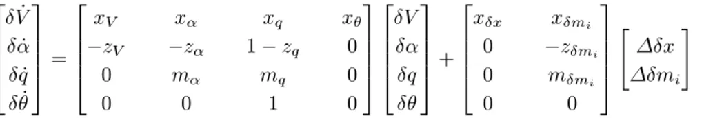
For control synthesis purpose, a linear state-space representation is obtained from Eq. 4 to 8 using finite differences method on different flight points. This state-space representation reads:
δ ˙V δ ˙α δ ˙q δ ˙θ = xV xα xq xθ −zV −zα 1− zq 0 0 mα mq 0 0 0 1 0 δV δα δq δθ + xδx xδmi 0 −zδmi 0 mδmi 0 0 " ∆δx ∆δmi # (9)
The states are δV , δα, δq, δθ, variations around an equilibrium of the airspeed, angle of attack, pitch rate, and attitude respectively. The different terms of all matrices are developed in the Appendix. Concerning the controls, ∆δx denotes the thrust command, and ∆δmi denotes the i-th control surface command, the
different control surfaces layouts being developped in Section II.B.2. II.B.2. Control Surfaces Layout
In this section three different control surfaces layouts are presented and their rationale is explained. The problem of number and spacing of trailing edge control surfaces for BWB was already pointed out by Garmendia et al16.18 They provided an extensive view on all currently studied BWB configurations
and controls layouts. Another study of interest was performed by Belschner:19 an optimisation was run
on failure cases considering electro-mechanical actuators (EMA) driving independant control surfaces. An optimal layout of 23 control surfaces resulted of the process. Failure case analysis is out of scope of our study, as is a sizing of a whole FCS. Rather we expect to rough out actuator dynamics, which would then serve as an input for a more precise FCS sizing.
The initial configuration evaluated here is visible on figure 3(a). Five control surfaces are spread along the half span, except a gap from elevon 1 to 2 — control surfaces are numbered from inboard to outboard — due to the presence of the engine pylon. The whole trailing edge of a BWB is usually devoted to control, as the lack of longitudinal lever arm should be compensated by large surfaces. On control surfaces 3, 4 and 5 the relative inboard and outboard chords were kept constant, so their absolute chords decrease due to the taper ratio of the outer wing. Their chords are moreover limited by a rear spar. The inboard chord of the second control is also limited by cargo and cabin considerations.
(a) Initial control surfaces lay-out.
(b) Iso-area layout. (c) Iso-inertia layout.
Figure 3. Control surfaces layouts evaluated.
From a static point of view, previous studies6 demonstrated that total control surfaces efficiency of this
configuration was sufficient to fulfill both longitudinal and lateral handling qualities requirements, provided all surfaces are used as multicontrol. Control allocation algorithms were implemented for that purpose.20
So to keep comparison as fair as possible, total area devoted to control surfaces is kept as close as possible to the reference configuration when evaluating alternative layouts.
From this point, two layouts were compared to the initial one in order to test the fast prototyping method presented here. Elevons number is kept constant. The most inboard elevon remained constant due to here-above mentioned constraints. Total span is still devoted to controls, only relative span — and chord when necessary — are changed. Two designs are presented here:
• an Iso-area design, visible on figure 3(b), where an equality constraint was set on control surfaces areas of 2, 3, 4 and 5. Relative chords of 3, 4 and 5 are set constant at 22%. Only the inboard chord of 2 has to be slightly decreased compared to the initial design in order to provide a feasible solution. The overall area is then a bit decreased.
• an Iso-inertia design, visible on figure 3(c), where total area is set equal to the initial total area in order to provide a feasible design. Then relative chords of 3, 4 and 5 are set as free parameters to fulfill the equality requirement on all control surfaces inertia with respect to their hinge.
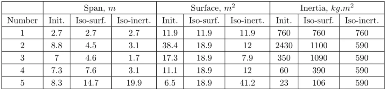
All three layouts geometrical characteristics are summarized in table 1. The most significant difference between the derived layouts and the initial one is that the largest elevon, which is initially inboard — namely elevon 2 — is now outboard — namely elevon 5 — particularly for the ”iso-inertia” design .
Span, m Surface, m2 Inertia, kg.m2
Number Init. Iso-surf. Iso-inert. Init. Iso-surf. Iso-inert. Init. Iso-surf. Iso-inert.
1 2.7 2.7 2.7 11.9 11.9 11.9 760 760 760
2 8.8 4.5 3.1 38.4 18.9 12 2430 1100 590
3 7 4.6 1.7 17.3 18.9 7.9 350 1090 590
4 7.3 7.6 3.1 11.1 18.9 12 60 390 590
5 8.3 14.7 19.9 6.5 18.9 41.2 23 106 590
Table 1. Control surfaces characteristics for three different layouts: initial, iso-surface and iso-inertia. Control surfaces are numbered from most inboard (1) to most outboard (5).
II.B.3. Aerodynamics of the Derived Layouts Computation
Aerodynamic model of the derived layouts is described in this section. For sake of clarity the initial layout is called ”reference” aircraft, and the two derived layouts —namely iso-area and iso-inertia layouts — are called ”project” aircraft. The reference flight dynamics model described in section II.B.1 is used for all three configurations from section II.B.2 as planform and airfoils are kept constant for all configurations; therefore only control surfaces aerodynamic efficiencies need to be evaluated for the two derived layouts. For that purpose the Athena Vortex Lattice (AVL) software21was used together with calibration factors coming from
the supposedly known aerodynamic coefficients of the initial BWB design.
More precisely the lift coefficient CL introduced in Eq.4 comprises a i-th control surface deflection
de-pendency CLi which can be written as:
CLi = k
N L
δmi(α, δmi)CLδmiδmi (10)
where kN L
δmi(α, δm) accounts for loss of control surface efficiency as a function of the angle of attack α and control surface deflection δmi, and CLδmi is the lift gradient of the i-th control surface. kδmN Li(α, δm) is known for reference aircraft, and kept for project aircraft. Reference lift gradient CLref
δmi is supposed known from previous studies, and is compared with the lift gradient computed by AVL for the reference configuration CLAV Lδmi (see figure 5(a)). From these data a calibration factor accounting for AVL lack of accuracy is computed:
∆CLAV Li = CLref δmi CAV L Lδmi (11) Then an AVL computation is run on project geometry in order to compute the lift gradient of project aircraft CAV Lproj
Lδmi . This gradient is finally calibrated using the previously computed calibration factor ∆CLAV Li of Eq.11 (see figure 5(b)), giving:
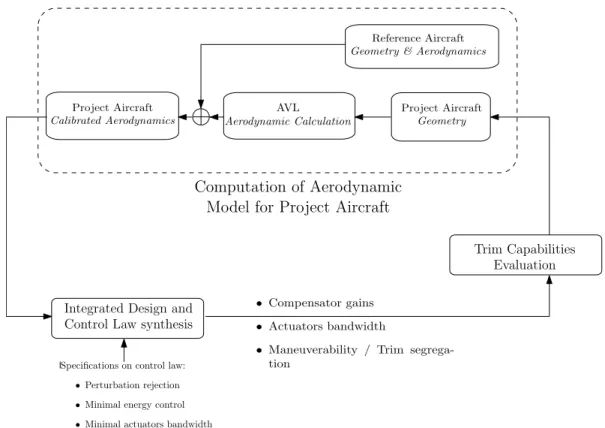
Reference Aircraft Geometry & Aerodynamics
Project Aircraft Calibrated Aerodynamics Project Aircraft Geometry AVL Aerodynamic Calculation
Computation of Aerodynamic
Model for Project Aircraft
Integrated Design and Control Law synthesis
Specifications on control law: • Perturbation rejection • Minimal energy control • Minimal actuators bandwidth
Trim Capabilities Evaluation
• Compensator gains • Actuators bandwidth
• Maneuverability / Trim segrega-tion
Figure 4. General process of the study including computation of aerodynamic model for project aircraft.
CLproji = kN Lδmi∆C
AV L Li C
AV Lproj
Lδmi δmi (12)
A similar process is used for computing control surfaces pitching moment efficiencies of project configu-rations. More precisely the lift coefficient Cm introduced in Eq.6 comprises a i-th control surface deflection
dependency Cmi which can be written as: Cmi= k
N L
δmi(α, δmi)CLδmiδmi(XCG− XFi) (13) where XCGdenotes the x−wise CG position, and XFi denotes the i-th control surface aerodynamic center x−wise position. However XFi is not a direct output of AVL and has to be computed as follows:
XFAV Li = XCG− CAV L mδmi CAV L Lδmi (14) This leads to computing the aerodynamic center calibration factor for the reference aircraft knowing the actual aerodynamic center XFrefi for the i-th elevon:
∆XFAV Li = XFrefi XAV L
Fi
(15) Finally an AVL computation is run on project aircraft in order to compute the pitching moment gradient of project aircraft i-th elevon CAV Lproj
mδmi , and the resulting aerodynamic center is computed and calibrated as
follows: XFAV Li proj = ∆X AV L Fi . XCG− CAV Lproj mδmi CAV Lproj Lδmi ! (16) This method, summarized on figure 4, combines the advantages of fast data generation through light CFD computation, and far better accuracy than AVL direct output through accurate knowledge on a reference configuration. Here it is applied only to control surfaces aerodynamic coefficients, but the process would be similar for computing any aerodynamic coefficient of a project aircraft with a baseline knowledge on a similar reference aircraft.
(a) Comparison of pitch gradient coefficients for reference aircraft: CLref
δmi (dotted) vs C AV L Lδmi (plain).
(b) Comparison of pitch gradient coefficients for project aircraft before and after calibration respectively: CLAV Lproj
δmi (plain) vs C proj
Lδmi (dotted) Projet aircraft here
is ”iso-area” layout.
Figure 5. Comparison of pitch gradient coefficientsCLδmi from AVL outputs with reference aircraft aerodynamic data (left) and with calibrated data (right). Indices denote elevon number.
III.
Integrated Design and Control
In this section the problem of integrated design and control is formulated. III.A. Plant-Controller Optimization General ProblemThe usual way of designing and stabilizing an aircraft is a sequential approach: first the aircraft is sized taking into account disciplines such as aerodynamics, weight, engine sizing, performance and open-loop han-dling qualities. Then when the overall aircraft design is mostly frozen control laws are designed in order to improve closed-loop handling qualities and passenger comfort, or to alleviate loads. The assumption for this sequential procedure is that the open-loop plant is adequately designed in order to guarantee good control performance. From an engineering point of view, this is generally true for classical tail-aft configurations, for this configuration was historically selected as being flyable without any control law. This is no more the case for BWB configuration. Also from a theoretical point of view, sequential plant-controller design was shown to lead to suboptimal configurations.22 The idea is then to simultaneously optimize the plant and controller
to achieve a globally optimal design. This problem, known in litterature as Plant-Controller Optimization, Integrated Design and Control or Co-Design, was adressed in different domains such as spacecraft design for controlling flexible appendages,23 chemistry24 and underwater vehicles.25 In aircraft design several
ap-proaches were investigated. Already in the 70s’ a study by the US Air Force showed the benefits of RSS for a control-configured vehicle in terms of operating weight empty (OWE) and gross weight (GW). More recently studies by Perez et al.26 incorporated a stability and control (S&C) module into a multidisciplinary
optimization (MDO) process, showing improved aircraft design over a traditional process. Another approach of interest consists in integrating plant relevant parameters into a controller optimization. Plant and con-troller parameters are then optimized simultaneously in the concon-troller optimization. Most formulations to our knowledge involve linear matrix inequalities (LMI) formulations of open and closed-loop handling quali-ties requirements. In the work of Niewoehner and Kaminer, a sequential optimization of control surfaces and controller is performed using LMI optimization for state-feedback controller27.28 More recent work of Liao
et al.29 involve H
∞plant-controller optimization also based on LMI for a single aircraft parameter, namely
the elevator size. This work is extended to mixed H2/H∞ control with optimization of several aircraft
parameters in a related study.30
sophisticated dynamic controllers require reduction techniques in order to be practically implementable. With recent advances in the field of nonsmooth optimization techniques for structured H∞ synthesis31,32
the problem of integrated design and control for spacecraft avionics was addressed using structured control laws and plant parameter by Alazard et al.33 Later this formulation was extended to aircraft design34 and gain-scheduling techniques.35 This structured controller approach is used in the present paper. Section III.B
formulates the control problem, and section III.C presents the co-design approach.
III.B. H2/H∞ Formulation for Perturbation Rejection on the Acceleration Sensitivity
Func-tion
First it is important to remind that the aim of this study is not to provide directly implementable control laws, rather a quick prototyping of control laws and control surfaces layouts for different configurations. Therefore static state feedback u =−K.[α q θ]T of the angle-of-attack, pitch rate and pitch angle respectively, is used.
This corresponds to some kind of augmented pitch damper: on most recent aircraft degraded control law feature only direct order of the pilot to control surfaces, in addition with a pitch rate feedback. However it was found that for such unstable configurations as the BWB pitch-rate feedback is not sufficient to properly stabilize the short-period oscillation. Therefore α and θ feedback were added, in order to add some feedback ”stiffness”. The u command vector is composed of ten elements: a different feedback order is sent to each of the ten control surfaces. This allows for a linear control allocation strategy of the control law optimizer: elevons are differently used according to their relative pitch efficiencies.
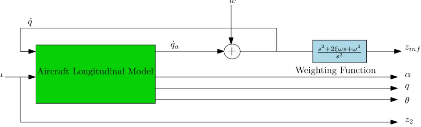
Aircraft Longitudinal Model
w s2+2ξωs+ω2 s2 zinf u z2 α q θ ˙qa ˙q Weighting Function
Figure 6. Standard problem of perturbation rejection of the acceleration sensitivity function
The control problem formulation is based on a H∞ weighting on the acceleration sensitivity function.
This approach is extensively described in work by Fezans et al.36 The rationale for using this approach in
our problem is the assumption that from a sizing point of view, perturbation rejection is more stringent than command tracking. In other words, it is harder to reject unknown disturbances than to follow known commands. Therefore we are focusing on perturbation rejection — ie stabilizing the aircraft while facing external disturbance such as turbulence — instead of command tracking such as maneuver response to pilot input. This assumption would deserve to be checked, however this is out of scope of the study.
We consider an unknown disturbance w that perturbates the aircraft pitch acceleration ˙qa, leading to a
resulting pitch acceleration ˙q = ˙qa+ w (see figure 6). This is equivalent to considering a disturbing moment
on pitch axis. The objective of the control law is then to limit the influence of perturbation w on closed-loop acceleration. In order to obtain the desired behaviour for closed-loop pitch acceleration a weighting function W1 = s
2+2ξωs+ω2
s2 is specified on resulting pitch acceleration ˙q. If this frequency template is fulfilled, the pitch motion will behave as a second-order system with specified damping ξ and pulsation ω. The H∞
constraint can now be written as follows:
kW1Tw→ ˙qk∞≤ γ∞ (17)
kk∞ being the H∞ norm, and γ∞being a value slightly above 1. In practice we will assume γ∞= 1.5.
However this problem is under-constrained, and without further specifications commands are allowed to raise to high values. To avoid this, a minimization objective is set on the H2 norm of the transfer between
the disturbance w and the command u. The mixed H2/H∞problem is then formulated as follows:
min
K kTw→uk2
subject to: kTw→zinfk∞ ≤ γ∞ (18)
zinf being defined on figure 6. In other words: over the set of controllers satisfying closed-loop
require-ments for perturbation rejection, choose solution with minimal control energy. III.C. Co-design on Actuators Bandwidth
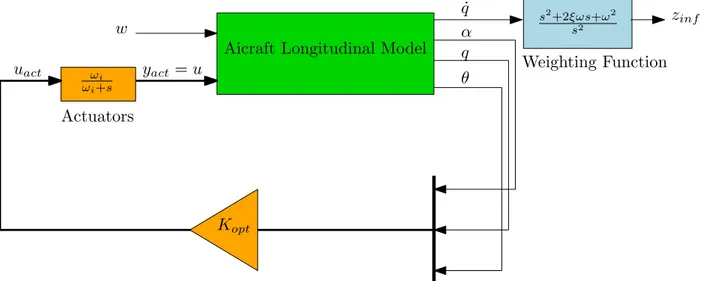
In section III.B the initial control problem was introduced. In this section the co-design problem is formu-lated. The formulation presented here was more extensively developed in previous studies.34
Aicraft Longitudinal Model
α
q
θ
ωi ωi+sActuators
w
z
infK
optu
acty
act= u
s2+2ξωs+ω2 s2Weighting Function
˙q
Figure 7. Closed-loop problem of integrated design and control of state-feedback and actuators bandwidth. Open-loop aircraft dynamics is represented in green, weighting function in blue and tunable parameters in orange.
Actuators dynamics of each elevon is now modelled by a first order transfer of the form: yact
uact
(s) = ωi ωi+ s
, i = 1...10 (19)
where yactand uactare the actuators output and input respectively, as defined on figure 7. ωirepresents the
i-th elevon bandwidth. This bandwidth is not a fixed parameter, but a variable which is optimized conjointly with control law synthesis. Ω = [ω1, . . . ω10]T is the vector of design parameters.
The aim of combined optimization is to minimise the actuators bandwidth required to properly stabilize the aircraft. Indeed as shown in section II, high actuators bandwidth lead to high deflection rates, as well as heavy and high power-consuming actuators. Moreover, smaller control surfaces should be allowed to move faster than bigger ones: therefore it was chosen to weight each bandwidth ωiby the associated control surface
inertia Jiwith respect to its hinge in the objective formulation. The objective function associated to aircraft
parameters is then: min Ω .. . Jiωi .. . ∞ = min Ω maxi |Jiωi|
subject to: 0≤ Ω ≤ Ωmax (20)
where Ωmax is an upper bound for actuators bandwidth, eg. Ωmax = 8Hz, and J = [J1, ...J10]T is a
vector of all control surfaces inertia. Finally the multiobjective optimization is written as a min-max of the two previously described objectives:
min
K,Ω maxi {
1
M axAmpkTw→uact(s, K)k2,|Jiωi|}
subject to:kTw→zinfk∞≤ γ∞, 0≤ Ω ≤ Ωmax (21) Please note that with the introduction of actuators dynamics the energy minimisation criterion acts no more on the transfer Tw→ubut on Tw→uact. This was done on purpose, so that the control energy objective
kTw→uact(s, K)k2 mostly affects the gains K and not the bandwidth Ω. Said shortly, kTw→uact(s, K)k2 is
concerned with minimizing values of K, and min max|Jiωi| is concerned with minimizing values of Ω. A
trade-off arises between K and Ω: same control performance may be achieved for higher gain values and smaller bandwidth and reciprocally.
In order to be compared and conjointly optimized, the two objective functions are normalized through the parameter M axAmp. This parameter has to be carefully chosen as it drives the trade-off between control and design requirements. Usually, in multi-objective control, design weights are seen only as degrees of freedom for the designer; no attention is paid on physical meaning of these weights. The situation here is different, for one of the objectives comprises physical variables. Therefore the weight M axAmp is calculated as follows:
M axAmp = k×kTw→uactk
0 2 kJΩ0k ∞ (22) where: • kTw→uactk 0
2 represents minimal energy control, computed with a linear quadratic (LQ) synthesis and
no actuators dynamics — ie infinite bandwidth. As this represents an ideal situation, optimal value of the multiobjective problem will necessarily be above this value.
• kJΩ0k
∞is the value of design objective for initial bandwidth, eg. Ω0= 3Hz. As we seek to mimimize
this criterion, optimal value will be below this value.
• k represents the factor which we are willing to loose on control energy optimality, in order to gain on actuators bandwidth. Therefore we want k≥ 1. Indeed in eq.(21) objectives are normalized to 1, so when optimality is reached following relation is obtained:
kTw→uactkopt2
kJΩkopt∞
= M axAmp (23)
So the k factor can be interpreted as:
k = kTw→uactk opt 2 kTw→uactk02 .kJΩ 0k ∞ kJΩkopt∞ (24) For this study we found that k = 5 is providing good results for all control surfaces layouts.
From an implementation point of view, we chose to work with the systune and slTunable37 routines
from MATLABTMfor:
• It allows mixed H2/H∞ synthesis and multiobjective optimization.
• It allows structured parameters.
• Bounds on the variables are easily applicable.
• Design and simulation model can be derived directly from a single block diagram file.
• Constraints specifications are not limited to specifications on frequencies, but may also handle pole placement constraints, which may be more suitable to handling qualities purpose. This is out of scope of the study but may be addressed in future work.
Finally this optimization was run on a single flight point, corresponding to the most sizing one from codesign procedure point of view. To find this sizing point, the process is run for the initial configuration on different flight points corresponding to different altitudes and Mach numbers. The sizing point is selected as being the flight point requiring maximal actuators bandwidth in order to stabilize the configuration with adequate performance. Interestingly, it was found that this sizing point, corresponding to a high-altitude low-speed flight point, does not correspond to the maximal absolute instability of the short period oscillation mode. Rather it combines a strong longitudinal instability with a lack of control surfaces efficiency due to low dynamic pressure.
IV.
Results
In this section, results of the optimization problem defined in section II and III are presented, and trim capabilities of the different configurations are evaluated.
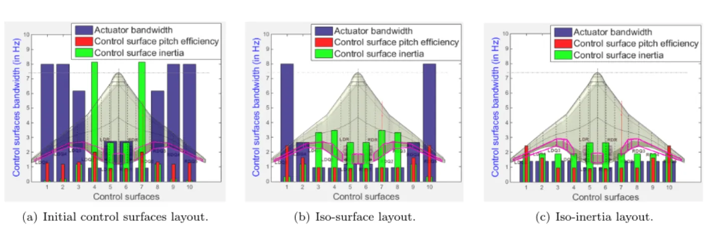
IV.A. Actuators Bandwidth Preliminary Sizing for Different Layouts
(a) Initial control surfaces layout. (b) Iso-surface layout. (c) Iso-inertia layout.
Figure 8. Control surfaces inertia (normalized), pitch efficiencies and actuators bandwidth preliminary sizing through integrated design and control procedure for different control surfaces layouts.
For each layout an optimization process is performed, and performance of the three layouts are discussed. On table 2 numerical values of some meaningful norms introduced in section III.C are presented before and after optimisation process, for the three evaluated layouts. Results are consistent with what was stated in section III.C:
• kTw→uactk2increases between initial (LQ without actuators dynamics) and optimal design. This means that gains have to be increased as we move away from an ideal situation in order to stabilize the aircraft with required performance.
• kJΩk∞ is decreased from initial to optimal design.
• kTw→zinfk
opt
∞ is below the γ∞value. This indicates that required performance specification is fulfilled
for all designs. This may also be seen on figure 9, where frequency responses of the three closed-loop layouts are plotted, as well as the W1template for performance specification. Frequency responses are
located below the weighting function W1, which indicates that performance is satisfied for all control
laws.
Looking at optimized actuators bandwidth on figure 8, some significant differences among different layouts are observed.
• Initial layout features three fast outboard control surfaces, corresponding to the three smallest elevons. Inboard elevons 1 and 2 have a slow dynamics.
• Iso-surface layout features one fast outboard elevon pair, and to a lower extend also elevon 4. All three inboard elevons feature slow dynamics.
Control surfaces layout Norms Initial Iso-area Iso-inertia kTw→uactk 0 2 0.8097 0.7496 0.7496 kJΩ0 k∞ 4.59.104 1.96.104 1.49.104 kTw→uactk opt 2 1.2684 1.1431 1.2415 kJΩkopt ∞ 1.43.104 5.98.103 4.96.103 kTw→zinfk opt ∞ 1.0836 1.0666 1.1755 Table 2. Different norms for initial and optimal parameters.
Figure 9. Frequency responses of Tw→zinf for initial (blue), iso-surface (green) and iso-inertia (red) layouts. W1
weighting function is also represented.
• Iso-inertia layout is the most balanced one, with only relatively low dynamics actuators. Small dif-ferences on numerical values are observed due to difference of pitch efficiencies of different elevons — outboard control surfaces having more x-wise lever arm— but this is second order.
Most important is that control synthesis provides a control architecture with guaranteed performance, for reasonable gains increase —60% increase from an H2norm perspective— from ideal to optimized design.
Resulting bandwidth are challenging but not unrealistic. Even though this study is too preliminary to draw some definitive conclusions, it seems that the initial layout is too unbalanced for being efficient, some elevons being very small and other very large.
IV.B. Evaluation of Trim Capabilities under Trim / Maneuverability Segregation Assump-tions
The co-design process presented in section IV.A gives some insight about a frequential allocation among control surfaces: it stipulates that in order to provide sufficient perturbation rejection performance, some control surfaces need to move very fast while some other are allowed to have slower dynamics. The former ones may be called ”maneuverability” control surfaces, while the latter ones may be called ”trim” control surfaces. While the co-design process states that maneuverability control surfaces are sufficient to properly stabilize the aircraft, it is not set yet whether remaining trim control surfaces are sufficient for equilibrating the aircraft. The main interest of such a trim / maneuverability segregation would be to use different actuators technologies for these two functions. Indeed it was shown by Garmendia et al.2 allocating only
trim to some elevons allowed for choosing irreversible actuators: hence no power penalty is paid in permanent flight once the control surface is deflected to its equilibrating position.
For the three layouts, trim control surfaces are selected as those with actuator bandwidth below 1Hz. For each configuration, elevons evaluated for trim are summarized in table 3.
Control surfaces layout Initial Iso-area Iso-inertia Elevons used for trim 1-2 1-2-3 1-2-3-4-5
Table 3. Control surfaces used for trim according to co-design results for the three layouts.
IV.B.1. Trim Criteria Description
CS-25 regulation states that it must be possible to trim the aircraft during every phase of the flight. Three relevant trim criteria are evaluated in this study: trim on glide, trim stall and trim turn.
1. Trim on glide: it must be possible to trim the aircraft on a 3◦glide path approach, for any combination
of mass and CG. To evaluate this criterion eq. (4) to (8) are solved at the equilibrium for different masses with following constraints:
• V = Vappthe approach speed.
• γ = −3◦ the flight path angle.
• δm = δmmin, respectively δm = δmmax, minimal, resp. maximal control surfaces deflection
allocated for trim.
Free variables to solve flight mechanics equations are: • F the thrust.
• α the angle of attack.
• XCGthe x−wise CG location.
Please note that in our formulation the CG is not restricted to its allowable locations, as defined on W &CG diagram of figure 2 for instance. Rather a minimal — upwards — trim control surfaces deflection is imposed, and maximal forward XCG position that such a deflection is able to balance
is computed. If this XCG position lies forward the allowable CG envelope, then trim elevons are
sufficiently efficient. Similarly a minimal —downwards — trim deflection leads to a backward XCG
position, which should lie backwards the allowable CG envelope.
2. Trim stall : The aircraft should remain trimmable and controllable near stall angle of attack, for any combination of mass and CG. Similarly to the trim on glide criterion, equilibrated flight mechanics equations are solved with following constraints:
• α = αstall the stall angle of attack.
• γ = 0◦.
• δm = δmmin, respectively δm = δmmax, minimal, resp. maximal control surfaces deflection
allocated for trim.
Free variables to solve flight mechanics equations are: • θ the pitch angle.
• V the air speed.
• XCGthe x−wise CG location.
3. Trim turn: this criterion is no more a pure longitudinal one. The aim of this criterion is to check the aircraft manoeuvrability in the following case: a coordinate turn at 45◦, landing speed and the
trim at minimum setting. Lateral flight dynamics equations are not described in this paper for sake of brevity, therefore only longitudinal constraints and free variables are listed below. However the actual equilibrium includes constraints on sideslip β, r and p yaw and roll rates respectively, and bank angle φ = 45◦. Longitudinal constraints are:
• γ = 0◦
• δm = δmmin minimal control surfaces deflection allocated for trim.
Longitudinal free variables to solve flight mechanics equations are: • F the thrust.
• α the angle of attack.
• XCGthe x−wise CG location.
On all evaluated layouts roll control is allocated to elevons 4 and 5. IV.B.2. Initial Control Surfaces Layout
(a) Weight and CG diagram for initial layout, with elevons 1 and 2 used for trim.
(b) Weight and CG diagram for initial layout, with all elevons used for trim.
Figure 10. Weight and CG diagrams for initial layout.
For the initial configuration and according to co-design results of figure 8(a), capacity of equilibrating the aircraft with only control surfaces 1 and 2 is evaluated. Results are presented on figure 10(a). It can be seen that trim on glide criterion is not challenging, for forward and backward limits respectively far exceed allowable CG positions. Same conclusion is valid for trim turn and trim stall forward criteria, which lie forward the W&CG diagram. However trim stall backward is not satisfied for some backward CG positions. Therefore a second computation is run using all elevons in for trimming the aircraft for this specific flight case. Indeed trim stall is a certification maneuver which needs to be performed with all trim capabilities. Results are presented on figure 10(b). Appart from all other criteria being relaxed, it is noteworthy that trim stall backward moved backward, as expected. However, for some specific combinations of mass and CG this criterion still lies inside the W&CG envelope. After investigations this means that αstall is not reached
for those backward configurations; nevertheless required CLmax is achieved thanks to CL contribution of positive deflections of the elevons for this flight case. This criterion is therefore considered as fulfilled. IV.B.3. Iso-Surface Control Surfaces Layout
Following what was presented in table 3, trim capacity of configuration iso-area is evaluated using elevons 1, 2 and 3 as trim devices. Results are presented on figure 11. One can see that all criteria are satisfied, except the trim stall backward criterion. As stated in section IV.B.2, this criterion allows for using all available control surfaces for trim. with such an allocation, the aircraft would be trimmable for backward CG at stall speed.
IV.B.4. Iso-Inertia Control Surfaces Layout
This last configuration features all control surfaces used both for maneuverability and trim, as presented on figure 8(c). Results of trim evaluation using all control surfaces are presented on figure 12. Once again all criteria but the trim stall backward are fulfilled. As stated previously the apparent lack of control efficiency for this maneuver comes from the formulation of the criterion, specifying a target αstall. However it was
Figure 11. Weight and CG diagram for ”iso-surface” layout, with elevons 1 2 and 3 used for trim.
checked that, taking into account CL contribution of positive deflections of the elevons, required CLmax is achieved at stall speed for backward CG.
Figure 12. Weight and CG diagram for ”iso-inertia” layout, with all elevons used for trim.
V.
Conclusion
A new method for fast prototyping of control surfaces actuators for unconventional unstable configura-tions is proposed. This method relies upon latest developments of nonsmooth optimization for structured controllers design. Stabilizing control law gains and actuators bandwidth are optimized in a single pro-cess. The result is guaranteed closed-loop performance as well as trim / maneuverability control surfaces segregation. In a last part of the study remaining capability of trim elevons is evaluated. The flexibility of the method is demonstrated through evaluation of three different control surfaces layouts for a blended wing-body. As a preliminary recommendation the authors suggest that control surfaces layouts with highly
different elevons sizes should be avoided, unless a segregation between maneuverability and trim is per-formed, as it is investigated in this paper. Therefore from this study the so-called ”iso-surface” layout seems promising compared to the initial one. Future work may include refined actuators modelling in order to assess relative weight and energy penalty for different configurations. Lateral control laws may also be in-cluded into the design process, for multi-control elevons may be sized by longitudinal-lateral maneuvers. A last study of interest would be to compare control surfaces layout with different number of elevons.
Appendix
Developing the coefficients in state-space matrices of section II.B.1 gives:
xV =−%V SCm x +∂V∂F, xα=−2gkCLα, xq =−2gLkV CLq, xθ=−g, zV =−2gV2 , zα= %V S 2m CLα, zq =%SL2mCLq, mα= %V2S B Cmα, mq =%V SL 2 2B Cmq, xδx= 1 m ∂F ∂δx, xδmi =−2gkCLδmi, zδmi = %V S 2m CLδmi, mδmi = %V2SL 2B Cmδmi
Acknowledgments
This work is part of a CIFRE PhD thesis in cooperation between ISAE-Supaero, ONERA and the Future Projects Office of Airbus Operations SAS.
References
1Roman, D., J. Allen, and R. Liebeck, “Aerodynamic Design Challenges of the Blended-Wing-Body Subsonic Transport,”
18th Applied Aerodynamics Conference, Fluid Dynamics and Co-located Conferences, American Institute of Aeronautics and Astronautics, Aug. 2000.
2Daniel C. Garmendia, Imon Chakraborty, and Dimitri N. Mavris, “Uncertainty Quantification for the Actuation Power
Requirements of a Hybrid Wing Body Configuration with Electrically Actuated Flight Control Surfaces,” 53rd AIAA Aerospace Sciences Meeting, AIAA SciTech, American Institute of Aeronautics and Astronautics, 2015.
3Liebeck, R., “Design of the Blended-Wing Body subsonic transport,” 2005-06, von Karman Institute for Fluid Dynamics,
June 2005.
4Zhoujie Lyu and Joaquim Martins, “Aerodynamic Shape Optimization of a Blended-Wing-Body Aircraft,” 51st AIAA
Aerospace Sciences Meeting including the New Horizons Forum and Aerospace Exposition, Aerospace Sciences Meetings, Amer-ican Institute of Aeronautics and Astronautics, Jan. 2013.
5Kozek, M. and Schirrer, A., Modeling and Control for a Blended Wing Body Aircraft , Springer, 2014.
6Saucez, M., Handling Qualities of the Airbus Flying Wing Resolution, PhD thesis, ISAE-Airbus, Toulouse, May 2013. 7Wildschek, A., “Flight Dynamics and Control Related Challenges for Design of a Commercial Blended Wing Body
Aircraft,” AIAA Guidance, Navigation, and Control Conference, AIAA, National Harbor, Maryland, Jan. 2014.
8Saucez, M. and Boiffier, J.-L., “Optimization of Engine Failure on a Flying Wing Configuration,” AIAA Atmospheric
Flight Mechanics Conference, Guidance, Navigation, and Control and Co-located Conferences, AIAA, Minneapolis, Minnesota, Aug. 2012.
9Roskam, J., Airplane flight dynamics and automatic flight controls, DARcorporation, 1995.
10Brinker, J. S. and Wise, K. A., “Flight Testing of Reconfigurable Control Law on the X-36 Tailless Aircraft,” JOURNAL
OF GUIDANCE, CONTROL, AND DYNAMICS , Vol. 24, No. 5, Oct. 2001.
11Rogers, W. L. and Collins, D. J., “X-29 H-infinity controller synthesis,” Journal of Guidance, Control, and Dynamics,
Vol. 15, No. 4, July 1992, pp. 962–967.
12Meheut, M., Arntz, A., and Carrier, G., “Aerodynamic Shape Optimizations of a Blended Wing Body Configuration for
Several Wing Planforms,” AIAA, Vol. 10, American Institute of Aeronautics and Astronautics, New Orleans, Louisiana, June 2012, p. 3122.
13Lyu, Z. and Martins, J. R. R. A., “Aerodynamic Design Optimization Studies of a Blended-Wing-Body Aircraft,” Journal
14Stein, G., “The practical, physical (and sometimes dangerous) consequences of control must be respected, and the
underlying principles must be clearly and well taught.” IEEE Control Systems Magazine, Vol. 272, No. 1708/03, 2003.
15Cameron, D. and Princen, N., “Control Allocation Challenges and Requirements for the Blended Wing Body,” AIAA,
Denver, CO, Aug. 2000.
16Daniel C. Garmendia, Imon Chakraborty, David R. Trawick, and Dimitri N. Mavris, “Assessment of Electrically Actuated
Redundant Control Surface Layouts for a Hybrid Wing Body Concept,” 14th AIAA Aviation Technology, Integration, and Operations Conference, AIAA Aviation, American Institute of Aeronautics and Astronautics, 2014.
17Meheut, M., Grenon, R., Carrier, G., Defos, M., and Duffau, M., “Aerodynamic design of transonic flying wing
configu-rations,” KATnet II: Conference on Key Aerodynamic Technologies, Bremen, Germany, 2009.
18Garmendia, D. C., Chakraborty, I., and Mavris, D. N., “Method for Evaluating Electrically Actuated Hybrid Wing Body
Control Surface Layouts,” Journal of Aircraft , April 2015, pp. 1–11.
19Belschner, T., “Definition of systems architecture for flight, load and vibration control of blended wing body type aircraft,”
MSc Thesis-Airbus Internal D3-21, EADS Innovation Works, Dec. 2011.
20Denieul, Y., “Control Allocation for multicontrol surfaces applied to unconventional aircraft configurations,” MSc
Thesis-Airbus Internal, Toulouse, France, Oct. 2013.
21Drela, M. and Youngren, H., “AVL-Aerodynamic Analysis, Trim Calculation, Dynamic Stability Analysis, Aircraft
Configuration Development,” Athena Vortex Lattice, Vol. 3, 2006, pp. 26.
22Fathy, H., Reyer, J., Papalambros, P., and Ulsov, A., “On the Coupling Between the Plant and Controller Optimization
Problems,” American Control Conference, 2001. Proceedings of the, Vol. 3, 2001, pp. 1864–1869 vol.3.
23Perez, J. A., Alazard, D., Loquen, T., Cumer, C., and Pittet, C., “Linear Dynamic Modeling of Spacecraft with
Open-Chain Assembly of Flexible Bodies for ACS/Structure Co-design,” Advances in Aerospace Guidance, Navigation and Control , edited by J. Bordeneuve-Guib, A. Drouin, and C. Roos, Springer International Publishing, Jan. 2015, pp. 639–658.
24Bansal, V., Ross, R., Perkins, J., and Pistikopoulos, E., “The interactions of design and control: double-effect distillation,”
Journal of Process Control , Vol. 10, No. 23, April 2000, pp. 219–227.
25Silvestre, C., Pascoal, A., Kaminer, I., and Healey, A., “Plant-Controller Optimization with Applications to Integrated
Surface Sizing and Feedback Controller Design for Autonomous Underwater Vehicles (AUVs),” Vol. 3, 1998.
26Perez, R. E., T. Liu, H. H., and Behdinan, K., “Multidisciplinary optimization framework for control-configuration
integration in aircraft conceptual design,” Journal of Aircraft , Vol. 43, No. 6, 2006, pp. 1937–1948.
27Niewhoener, R. J. and Kaminer, I., “Linear matrix inequalities in integrated aircraft/controller design,” American Control
Conference, Proceedings of the 1995 , Vol. 1, IEEE, 1995, pp. 177–181.
28Niewoehner, R. J. and Kaminer, I., “Integrated aircraft-controller design using linear matrix inequalities,” Journal of
guidance, control, and dynamics, Vol. 19, No. 2, 1996, pp. 445–452.
29Liao, F., Lum, K. Y., and Wang, J. L., “An LMI-based optimization approach for integrated plant/output-feedback
controller design,” American Control Conference, 2005. Proceedings of the 2005 , IEEE, 2005, pp. 4880–4885.
30Liao, F., Lum, K. Y., and Wang, J. L., “Mixed H
2/H∞Sub-Optimization Approach for Integrated Aircraft/Controller
Design,” presenting in the 16th IFAC World Congress, Prague, Czech Republic, 2005.
31Apkarian, P., Noll, D., Rondepierre, A., and others, “Nonsmooth optimization algorithm for mixed H
2/H∞ synthesis,”
Proc. of the 46th IEEE Conference on Decision and Control , 2007, pp. 4110–4115.
32Gahinet, P. and Apkarian, P., “Structured Hinfinity synthesis in Matlab,” IFAC World Congress, Universit Cattolica del
Sacro Cuore, Milano, Italy, 2011.
33Daniel Alazard, Thomas Loquen, Henry de Plinval, and Christelle Cumer, “Avionics/Control co-design for large flexible
space structures,” AIAA Guidance, Navigation, and Control (GNC) Conference, Guidance, Navigation, and Control and Co-located Conferences, American Institute of Aeronautics and Astronautics, Aug. 2013.
34Denieul, Y., Bordeneuve, J., Alazard, D., Toussaint, C., and Taquin, G., “Integrated Design and Control of a Flying
Wing Using Nonsmooth Optimization Techniques,” Advances in Aerospace Guidance, Navigation and Control , edited by J. Bordeneuve-Guib, A. Drouin, and C. Roos, Springer International Publishing, Jan. 2015, pp. 475–489.
35Lhachemi, H., Saussi, D., and Zhu, G., “A structured -based optimization approach for integrated plant and self-scheduled
flight control system design,” Aerospace Science and Technology, Vol. 45, No. 0, Sept. 2015, pp. 30–38.
36Fezans, N., Alazard, D., Imbert, N., and Carpentier, B., “H
∞control design for generalized second order systems based on
acceleration sensitivity function,” Control and Automation, 2008 16th Mediterranean Conference on, June 2008, pp. 1508–1513.