To link to this article :
DOI:10.1016/j.artint.2016.09.001
URL :
http://dx.doi.org/10.1016/j.artint.2016.09.001
To cite this version :
Bessière, Christian and Fargier, Hélène and
Lecoutre, Christophe Computing and restoring global inverse
consistency in interactive constraint satisfaction. (2016) Artificial
Intelligence, vol. 241. pp. 153-169. ISSN 0004-3702
O
pen
A
rchive
T
OULOUSE
A
rchive
O
uverte (
OATAO
)
OATAO is an open access repository that collects the work of Toulouse researchers and
makes it freely available over the web where possible.
This is an author-deposited version published in :
http://oatao.univ-toulouse.fr/
Eprints ID : 17214
Any correspondence concerning this service should be sent to the repository
administrator:
[email protected]
Computing
and
restoring
global
inverse
consistency
in
interactive
constraint
satisfaction
✩
Christian Bessiere
a,
Hélène Fargier
b,
Christophe Lecoutre
c,∗aLIRMM-CNRS,UniversityofMontpellier,France bIRIT-CNRS,UniversityofToulouse,France cCRIL-CNRS,UniversityofArtois,France
a b s t r a c t
Keywords:
Constraintsatisfactionproblems Configuration
Globalinverseconsistency
Someapplicationsrequire theinteractiveresolutionofaconstraint problembya human user. In such cases, it is highly desirable that the person who interactively solves the problem isnot given the choice to select values that do not lead to solutions. We call thispropertyglobalinverseconsistency.Existingsystemssimulatethiseitherbymaintaining arcconsistency after eachassignmentperformedby theuseror by compilingofflinethe problemas a multi-valued decision diagram. Inthis article,we define several questions relatedtoglobalinverseconsistencyandanalyzetheircomplexity.Despitetheirtheoretical intractability, we propose several algorithms for enforcing and restoring global inverse consistency and we show that the best version is efficient enough to be used in an interactivesettingonseveralconfigurationanddesignproblems.
1. Introduction
Constraint Programming (CP) iswidelyused toexpress and solvecombinatorial problems.Once a problem ismodeled asaconstraintnetwork,efficientsolving techniquesgenerate asolutionsatisfyingtheconstraints,ifsuchasolutionexists. However, thereare situations where theuser has strong opinions about the wayto build good solutions to the problem but someofthedesirable/undesirablecombinationswillbecomeclearonly oncesomeofthevariablesareassigned.Inthis case, the constraint solver should bethere to assist the user in thesolution design and to ensureher choices remain in the feasible space,removing thecombinatorial complexity from her shoulders. See theSynthia system for proteindesign as anearly example ofusing CP to interactivelysolve a problem[2]. Another wellknown example of such aninteractive solvingofconstraint-basedmodelsisproductconfiguration[3,4].Thepersonmodelingtheproductasaconstraintnetwork for thecompany knowsitstechnical and marketingrequirements. Shemodelsthefeasibility, availability and/ormarketing constraints abouttheproduct.Thisconstraintnetworkcapturesthecatalogofpossibleproducts,whichmaycontainbillions ofsolutions,butinanintentionalandcompactway.Nevertheless,themodelerdoesnotknowtheconstraintsorpreferences ofthecustomer(s).Thisisthecustomerwhowilllookforsolutions,withherownconstraintsandpreferencesontheprice, thecolor,orany otherconfigurablefeature.
✩ This paper isan invited revision of a paper whichfirst appeared at the 18th International Conference on Principles and Practice of Constraint
Programming(CP 2013)[1]. Thisarticle additionally containsa newsection on restoringglobal inverseconsistency aftertheretraction of a decision fromtheuser.Italsocontainsadditionalexperiments.
*
Correspondingauthor.Theseapplicationsrefertoaninteractivesolvingprocesswheretheuserselectsvaluesforvariablesaccordingtoherown preferencesand thesystemchecks theconstraints ofthenetwork,until allvariablesareassignedandsatisfyallconstraints of thenetwork.This solvingpolicy raises animportant issue:theperson whointeractively solvestheproblemshould not be led to a dead-end where satisfying all constraints of the network is impossible. Existing interactive solving systems address thisissue eitherbycompiling theconstraintnetwork intoamulti-valueddecisiondiagram(MDD)atthemodeling phase[4–6]orbyenforcingarcconsistencyonthenetworkaftereachassignmentperformedbytheuser[2].Compilingthe constraint network asan MDDcan require asignificantamount oftime and space.That iswhy compilationis performed offline (before thesolving session). As a consequence, configurators basedon an MDD compilation arerestricted to static constraintnetworks:non-unaryconstraintscanneitherbeaddednorremovedonce thenetwork iscompiled.Itisthus not possiblefortheusertoperformcomplexrequirements,e.g.sheisinterestedintravelingtoVeneziaonlyduringthecarnival period. Arcand dynamicarcconsistencies requirealightercomputationaleffortbut theusercanbetrapped indead-ends, which isvery riskyfromacommercialpointofview.Ithas beenshownin[7]that arcconsistency(andeven higherlevels of local consistency)canbe very badapproximationsof theideal statewhere allvalues remaininginthenetwork can be extendedtosolutions.
Themessageofourarticleisthatformanyoftheproblemsthatrequireinteractivesolvingoftheproblem,andespecially forrealproblems,itiscomputationallyfeasibletomaintainthedomainsofthevariablesinastatewheretheyonlycontain those valueswhichbelong toacompletesolution extendingthecurrent choices oftheuser.Inspiredbythenomenclature used in[8]and [9],wecallthislevelofconsistencyglobalinverseconsistency (GIC).
Our contribution addresses several aspects. First, we formally characterize the questions that underlie the interactive constraint solving loop and we show that they are all NP-hard. Second, we provide several algorithms with increasing sophistication to address thosetasks. Third, we experimentally show that themost efficient of ouralgorithms is efficient enoughtobeusedinaninteractiveconstraintsolvingloopofseveralnon-trivial configurationanddesign problems. 2. Background
A(discrete)constraintnetwork(CN)N iscomposedofafinitesetofn variables,denotedbyvars(N),andafinitesetofe
constraints,denotedbycons(N).Eachvariablex hasadomainwhichisthefinitesetofvaluesthatcanbeassignedtox.The initial domain ofavariable x is denotedbydominit(x) whereas thecurrent domainof x isdenoted bydom(x); wealways havedom(x)⊆dominit(x).Sometimes,weusedomN(x)todenotethedomainofx inthecontextoftheCNN.Themaximum domain sizeofavariableinagiven CNisdenotedbyd.Tosimplify, avariable–valuepair(x,a) suchthat x∈vars(N) and
a∈domN(x) is called avalue of N;we note values(N)= {(x,a)|x∈vars(N)∧a∈domN(x)}. Each constraint c involves
anordered set ofvariables,calledthescope of c anddenoted byscp(c),and issemanticallydefined byarelation, denoted byrel(c),which containstheset oftuplesallowed for thevariablesinvolvedin c.Thearity ofaconstraint c isthesizeof
scp(c),and willusuallybedenotedbyr.
Aninstantiation I ofaset X= {x1,. . . ,xk} ofvariablesisaset {(x1,a1), . . .,(xk,ak)}suchthat∀i∈1..k,ai∈dominit(xi); X isdenotedbyvars(I)andeachaiisdenotedbyI[xi].AninstantiationI on aCNN isaninstantiationofaset X⊆vars(N);
itiscomplete ifvars(I)=vars(N). I isvalid on N iff∀(x,a)∈I,a∈dom(x). I covers aconstraintc iffscp(c)⊆vars(I),and I satisfies aconstraintc withscp(c)= {x1,. . . ,xr}iff(i)I coversc and(ii)thetuple(I[x1],. . . ,I[xr])∈rel(c).Aninstantiation I on aCN N islocallyconsistent iff(i)I isvalidon N and(ii)every constraintof N coveredby I issatisfiedby I .Asolution
of N is acompletelocally consistentinstantiationon N; sols(N) denotestheset ofsolutionsof N. ACN N issatisfiable iff sols(N)6= ∅.
The ubiquitous example of constraint propagation is enforcement of generalizedarcconsistency (GAC) which removes values from domains without reducing the set of solutions of the constraint network. A value (x,a) of a CN N is GAC on N iff for every constraint c of N involving x, there exists a valid instantiation I of scp(c) such that I satisfies c and I[x]=a. N is GACiffevery valueof N is GAC.EnforcingGAC meansremoving GAC-inconsistentvaluesfromdomainsuntil theconstraintnetworkisGAC.Inthisarticle,weshallrefertoMACwhichisanalgorithmconsideredtobeamongthemost efficient genericapproachesfor thesolutionofCNs. MAC [10]exploresthesearchspacedepth-first,enforces(generalized) arc consistency after each decision taken (variable assignment or value refutation) during search, and backtracks when failures happen. A past variable is a variable explicitly assigned by the search algorithm whereas a future variable is a variablenot(explicitly)assigned.Theset offuturevariablesofaCNN isdenotedby varsf ut(N).
3. Problemsraisedbyinteractiveconstraintsolving
Inthissection,weformallycharacterizethequestionsthatunderlietheinteractiveconstraintsolvingloopandwestudy theirtheoreticalcomplexity.
3.1. Formalization
Wefirstdefinethelevel oflocalconsistencythat isdesirableinanyinteractive solvingloopinvolvingahuman,that is, thelevel ofconsistencythat guaranteesthatallvaluesinalldomainsbelongtoasolution.Inthenomenclatureintroduced by Freuder in [11] it corresponds to (1,n−1)-consistency if the constraint network contains n variables. To avoid the
reference to n, Freuder has called it variable completability in [12], and Dechter has called it globalconsistencyofvalues
in[13].To beconsistent withthenowwidelyaccepted nomenclatureintroducedin[8],we decidedtocallit globalinverse consistency.
Definition1(GlobalInverseConsistency). Avalue (x,a) ofaCNN isgloballyinverseconsistent(GIC) iff∃I∈sols(N)|I[x]=a.
ACN N is GICiffevery valuein values(N) isGIC.The GICclosure ofaCN N is theCNobtainedfrom N by removingall thevaluesthatdonotbelongtoasolutionofN.
We can observe that, as usual for levels of consistency, the GIC closure of a constraint network has the same set of solutionsastheoriginalnetwork.
There isa closerelationship between GIC and minimalityofconstraint networks asdefined byMontanari [14].A con-straint network is minimal according to Montanari if and only if any locally consistent instantiation of length 2 can be extendedtoasolution.Minimalnetworksareonlydefinedforbinary networks,thatis,whenthearityofallconstraintsis 2. Despite similarities in thedefinitionsof GIC and minimalnetworks—theyare bothbased on thenotion ofextensibilityto solutions,abinaryconstraintnetworkcanbeGICandnotminimalorminimalandnotGIC.Takeforinstancetheconstraint networkwithdom(x1)=dom(x2)= {1,2,3}andthesingleconstraintx1·x2=3.Itisobviouslyminimal,butitisnotGIC
be-cause2doesnotbelongtoanysolution.Takenowtheconstraintnetworkwithdom(x1)=dom(x2)=dom(x3)= {1,2,3}and
theconstraints x1+x2=4,x2+x3=4,and |x1−x3|≤1.ItisGIC,but itisnot minimalbecausethetuple ((x1,2),(x3,1))
isacceptedbytheconstraint|x1−x3|≤1 anddoesnotextendtoany solution.
The obviousproblems that follow from thedefinition ofGIC are tocheck whether a constraintnetwork is GIC ornot, and toenforceGIC.
Problem1(DecidingGIC).GivenaCNN,isN GIC?
Problem2(ComputingGIC).GivenaCN N,computetheGICclosure ofN.
As we are interested in interactive solving, we definethe problem of maintaining GIC after the user has performed a variableassignmentor,moregenerally,addedany arbitraryconstraint.
Problem3(MaintainingGIC).GivenaCNN thatisGIC,andaconstraintcne w withscp(cne w)⊆vars(N),recomputeGICafter theadditionofcne w tocons(N).
WealsodefinetheproblemofrestoringGICaftertheuserhasdecidedtodiscard anexistingconstraint.
Problem4(RestoringGIC).GivenaCNN anditsGICclosure NG I C,givenaconstraintc∈cons(N),recomputetheGICclosure
of N aftertheretractionofc from cons(N).
Inaconfiguration setting,assoonassome mandatoryvariableshave beenset, theuser canaskforan automatic com-pletionoftheremainingvariables.Hencethedefinitionofthefollowingproblem:
Problem5(SolvingaGICnetwork).GivenaCNN thatisGIC,findasolutionto N. 3.2. Complexityresults
Notsurprisingly, thebasicquestionsrelatedtoGIC(Problems 1 and2)areintractable.
Theorem1(Problem 1).DecidingwhetheraconstraintnetworkN isGICisNP-complete,evenifN issatisfiable.
Proof. We first prove membership toNP. For eachvalue (x,a) of N, itis sufficientto providea solution I of N such that theprojection I[x]of I onvariablex isequaltoa.Thiscertificatehassizen·n·d andcanbecheckedinpolynomialtime.
Completeness for NP is proved by reducing 3Col1 to the problem of deciding whether a satisfiable CN is GIC. Take
any instance ofthe 3Col problem, that is, a graph G= (V,E), and denote the threecolors by 1,2,3.Consider the CN N
where vars(N)= {xi|i∈V},dom(xi)= {0,1,2,3},∀i∈V ,andcons(N)= {(xi6=xj)∨ (xi=0∧xj=0)| (i,j)∈E}.Clearlythe
assignment {(xi,0)|i∈V}isasolutionof N,so N is satisfiable.If N isGICthenG is3-colorablebecause,byconstruction, N has solutions other than {(xi,0)|i∈V} iff G is 3-colorable. If G is 3-colorable then for any variable xi, there exists a
1 Thegraph3-colorabilityproblem(3Col)aimsatdecidingwhethertheverticesofagraphcanbecoloredbyusingthreecolorssuchthatnoedgelinks twoverticeshavingthesamecolor.
solution of N in which xi is assigned avalue in 1,2,3. Byswapping 1 with2, 2with 3and 3with 1on all variablesof thissolution,we stillhaveasolution.Similarlybyswapping1with3,2with 1and 3with2on allvariables.Thus,if G is
3-colorable thenN isGIC.Therefore,N isGICiffG is 3-colorable. ✷
Our proof shows that hardness for deciding GIC holds for binary CNs (i.e., CNs only involvingbinary constraints). We have another proof, inspired from that used in Theorem 3in [15], that shows that deciding GIC is still hard for Boolean domainsandquaternary constraints.
Theorem2(Problem 2).ComputingtheGICclosureofaconstraintnetworkN isNP-hardandNP-easy,evenifN issatisfiable.
Proof. We prove NP-easinessby showingthat a polynomialnumber ofcallsto aNP oracle aresufficient to buildtheGIC closure of N. Foreachvalue (x,a) ofN, weasktheNP oraclewhether N withtheextraconstraint x=a issatisfiable (we call thisaninversecheck).Once allvalues havebeen tested,we buildtheGIC closure of N by removingfrom eachdom(x) allvaluesa forwhichtheoracle testreturned‘no’.HardnessisadirectcorollaryofTheorem 1. ✷
NoticethatthetwopreviousintractabilityresultsarestillvalidwhentheCNissatisfiable,asisthecaseatthebeginning ofaninteractiveresolutionsession.
WefinallyshowthatProblems 3, 4 and5areunfortunatelynoteasierthanchecking GICorenforcingGICfromscratch. Buttheyarenotharder.
Theorem3(Problem 3).GivenaCNN thatisGIC,andaconstraintcne w withscp(cne w)⊆vars(N),computingtheGICclosureof theCNN′,wherevars(N′)=vars(N)andcons(N′)=cons(N)∪ {cne w}isNP-hardandNP-easyevenifcne w issimplyavariable assignmenty=b.
Proof. NP-easiness isproved as inthe proof of Theorem 2 byshowing that a polynomial number ofcalls to a NP oracle are sufficient to build the GIC closure of N′. For eachvalue (x,a) of N we ask theNP oracle whether N′ with theextra constraint x=a is satisfiable. Once allvalues have been tested,we build the closure of N′ by removing from dom(y) all valuesa6=b andremoving fromeachdom(x)allvaluesa forwhichtheoracle testreturned‘no’.
We prove hardness by reducing 3Col to the problem of computing the GIC closure of a GIC network after a variable assignment.Take anyinstanceofthe3Col problem,thatis,agraphG= (V,E),anddenotethethreecolors by1,2,3. Con-sidertheconstraintnetwork N wherevars(N)= {xi|i∈V}∪ {y1,y2},dom(xi)= {0,1,2,3},∀i,dom(y1)=dom(y2)= {0,1}.
cons(N)= {c(xi,xj)| (i,j)∈E}∪ {c′(xi,y1,y2)|i∈1..n}, withc(xi,xj) satisfiediff (xi6=xj∨xi=xj=0) and c′(xi,y1,y2)
satisfied iffat mosttwo variablesamong xi,y1 and y2 areassigned 0. N isGIC becausefor any i∈1..n, theinstantiation
where xi isassignedanyofitsvalues, xj=0,∀j6=i,and y1 and y2take0and 1orviceversa,isasolution.
Wereducethe3Col problemtotheproblemofenforcingGIConthenetworkN′withvars(N′)=vars(N)andcons(N′)=
cons(N)∪ {y1=0}.LetdomG I C bethedomainoftheGICclosureofN′.IfG is3-colorablethenassigningallxi’stoasolution
ofthe3-coloringand y2=0 isasolutionof N′.If0∈domG I C(y2),then y2=0 mustbelongtoasolution,says.xi’scannot
take value 0 in s otherwise constraints c′(x
i,y1,y2) would be violated. Thus, the restriction of s to xi’s variables is a
3-coloring. Therefore,G is3-colorableiff0∈domG I C(y2). ✷
Theorem4(Problem 4).GivenaCNN,itsGICclosureNG I C,andaconstraintcold∈cons(N),computingtheGICclosureoftheCNN′, wherevars(N′)=vars(N)andcons(N′)=cons(N)\ {cold}isNP-hardandNP-easyevenifcoldissimplyavariableassignmenty=b.
Proof. NP-easinessisproved asin theproofofTheorem 2.We provehardnessbyreducing 3Col totheproblemoftaking a network N for which we knowthe GICclosure NG I C, and computing the GIC closure ofthe network N′ obtained from
N by retracting a variable assignment. Take any instance ofthe 3Col problem, that is, a graph G= (V,E). Consider the constraint network N where vars(N)= {xi|i∈V}∪ {y}, dom(xi)= {0,1,2,3},∀i, dom(y)= {0,1}. cons(N)= {c1(xi,xj)|
(i,j)∈E}∪ {c2(xi,y)|i∈1..n}∪ {y=0},withc1(xi,xj) satisfiediff(xi6=xj)∨ (xi=xj=0) and c2(xi,y) satisfied iff(xi= y=0)∨ (xi6=0∧y6=0).Theonly solutionistheassignmentwhereevery xi isassigned0and y is assigned0.Thus, NG I C
has thedomaindomG I C definedbydomG I C(xi)= {0},∀i,anddomG I C(y)= {0}.
We show that the 3Col problem can be decided polynomially if we have anoracle enforcing GIC on the network N′
with vars(N′)=vars(N) and cons(N′)=cons(N)\ {y=0}.Let dom′
G I C bethedomainoftheGIC closure of N′.If G isnot
3-colorable then,byconstructionofc1 andc2, theonlysolutionisthesameasinN, that is,thetuple containingonly0’s.
If Gis3-colorable thenassigning asolutionofthe3-coloringtothexi’sand 1to y is asolutionof N′.Therefore, knowing
NG I C doesnothelp and G is3-colorableiff1∈domG I C(y). ✷
Theorem5(Problem 5).GeneratingasolutiontoaGICconstraintnetworkcannotbedoneinpolynomialtime,unlessP=N P .
Algorithm 1: GIC1(N:CN). 1 foreach variablex∈varsf ut(N)do 2 foreach valuea∈dom(x)do 3 I←searchSolutionFor(N|x=a) 4 if I=nil then
5 removea fromdom(x)
Algorithm 2: handleSolution2/3(x:variable, I :instantiation). 1 foreach variabley∈varsf ut(N)suchthat y isrevisedafterx do
2 ifstamp[y][I[y]]6= timethen 3 stamp[y][I[y]]← time 4 nbGic[y]++
Algorithm 3: isValid( X :setofvariables,I :instantiation):Boolean. 1 foreach variablex∈X do
2 if I[x]∈/dom(x)then 3 return false 4 return true
Suppose we have an algorithm A that generates a solution to a GIC constraint network N in time bounded by a polynomial p(|N|). Take any instance of the 3Col problem, that is, a graph G= (V,E). Consider the CN N where vars(N)= {xi|i∈V}, dom(xi)= {1,2,3},∀i∈V , and cons(N)= {xi6=xj| (i,j)∈E}. N hasa solution iff G is 3-colorable.
Now, if G is3-colorable thenN is GICbecauseanypermutationofthethreecolorsappliedtoallvariablesremainsa solu-tion(as intheproofofTheorem 1).Thus,itissufficienttorun A duringp(|N|)steps.Ifitreturnsasolutionto N,thenthe 3Col instance is satisfiable. Otherwise, the 3Col instance isunsatisfiable. Therefore, as3Col is NP-complete,there cannot exist apolynomialalgorithmforgenerating asolutiontoaGICconstraintnetwork,unless P=N P . ✷
4. Algorithmsforenforcing/maintainingGIC
Inthissection,weintroducefouralgorithmstoenforceglobalinverseconsistency.TheseGICalgorithmsuseincreasingly sophisticated data structures and techniques that have recently proved their worth in propagation algorithms proposed in the literature. To simplify our presentation, we assume that the CNs are satisfiable, which is the case in interactive resolution, allowingustoavoid handlingdomainwipe-outsintheGICprocedures. Notethat thesealgorithmscanbeused to enforce GIC, but also to maintain it during a user-driven search. This is why we referto theset varsf ut(N) of future variablesinsomeinstructions.
The first algorithm, GIC1, is similar to an algorithm proposed in [18]. GIC1 is described in Algorithm 1. It is really basic: it will be used as our baseline during our experiments. For each value a in the domain of a future variable x, a solution for the CN N where x is assigned the value a, denoted by N|x=a, is sought using a complete search algorithm.
Thissearchalgorithm,calledhere searchSolutionFor,eitherreturnsthefirstsolutionthat canbefound,orthespecial value
nil.Our implementationchoicewill bethealgorithm MAC that maintains(G)AC duringa backtracksearch[10]. Hence,in
Algorithm 1, whenitisprovedwith searchSolutionFor that nosolution exists,i.e. I=nil,thevalue a canbedeleted. Note that, incontrary toweakerformsofconsistency, whenavalue isprunedthereisnoneedforGIC torepeat theprocessof iterating overthevaluesremainingintheCN.
Thesecondalgorithm, GIC2described inAlgorithm 4(ignoringlightgreylines), usestimestamping.Thisisusefulwhen GIC is maintained during a user-driven search. We use an integer variable time for counting time, and we introduce a two-dimensional array stamp that associates with each value (x,a) of the CN the last time (value of stamp[x][a]) a solution was found for that value (0, initially). We also assume that variables areimplicitly totally ordered (forexample, in lexicographic order). Then, the idea is to increment the value of the variable time whenever a new call to GIC2 is performed(seeline1)andtotesttimeagainsteachvalue(x,a)oftheCN(seeline5)todeterminewhetheritisnecessary ornottosearchforasolutionfor(x,a).Whenasolution I isfound,function handleSolution2/3 iscalledatline10inorder to updatestamps.Actually, weonlyupdate thestamps ofvaluesin I correspondingtovariablesthat areprocessed afterx
intheloopofrevisions(line4) inAlgorithm 4.Thesearethevariablesthathavenotbeenprocessedyet bytheloopatline 4ofAlgorithm 4.Finally,byfurtherintroducingaone-dimensionalarraynbGicthatassociateswitheachvariablex ofthe CNthenumberofvalues indom(x) thathave been provedtobeGIC, itispossibleto avoidsome iterations ofloop5;see initializationatlines 2–3,testingatline4andupdateatline4ofAlgorithm 2.
The thirdalgorithm, GIC3, described in Algorithm 4 when considering lightgrey lines, can beseen asa refinementof GIC2 obtained byexploitingresidues, which correspond to solutionsthat have been previously found. Here,we introduce
Algorithm 4: GIC2/3(N:CN).
// GIC3 is obtained by considering light grey colored instructions between lines 5 and 6, and after line 10
1 time++
2 foreach variablex∈varsf ut(N)do 3 nbGic[x] ←0
4 foreach variablex∈varsf ut(N)suchthatnbGic[x] < |dom(x)|do 5 foreach valuea∈dom(x)suchthatstamp[x][a]< timedo
if isValid(vars(N),residue[x][a]) then handleSolution2/3(x,residue[x][a]) continue
6 I←searchSolutionFor(N|x=a) 7 if I=nil then
8 removea fromdom(x)
9 else
10 handleSolution2/3(x,I )
residue[x][a]←I
Algorithm 5: handleSolution4(I :instantiation). 1 foreach variablex∈Ssupdo
2 if I[x]∈ gicValues[/ x]then
3 gicValues[x]← gicValues[x]∪ {I[x]} 4 if|gicValues[x]|= |dom(x)|then 5 Ssup←Ssup\ {x}
a two-dimensional array residue that associates with eachvalue (x,a) ofthe CNthe last solution found for this value (potentially, during another call to GIC3). Because residual solutions may not be valid anymore, for each value (x,a) we need to test the validity of residue[x][a] bycalling thefunction isValid; seeinstructions between lines 5 and 6. If the residue isvalid,wecall handleSolution2/3 toupdatetheotherdatastructures,and wecontinue withthenextvalueinthe domain of x.A validity test, Algorithm 3, only checks that allvalues in agiven complete instantiationare still present in thecurrentdomains.Ofcourse,whenanewsolutionisfound,werecorditasaresidue;seeinstructionafter line10.
Our last algorithm, GIC4 described in Algorithm 6, is based on an original use of simple tabular reduction [19]. The principle istorecordallsolutions foundduringtheenforcementofGIC inatable, sothat an(adaptationofan) algorithm suchasSTR2[20]canbeapplied.Thecurrenttableisgivenbyallelementsofanarraysolutions atindicesrangingfrom 1 to nbSolutions. As for STR2,we introduce two sets of variablescalled Sval and Ssup. The former allowsus to limit validity control ofsolutions to thevariables whosedomains have changed recently(i.e., sincethe last executionofGIC4). Thisismadepossiblebyreasoningfromdomaincardinalities,asperformedatlines3and26–27withthearraylastSize. The latter (Ssup)contains any future variable x forwhich at least one value isnot in thearray gicValues[x],meaning that it has still tobeproved GIC.Related detailscanbefound in [20]. Aftertheinitializationof Sval and Ssup (lines1–8),
eachinstantiationsolutions[i] ofthecurrenttableisprocessed(lines 11–16).Ifitremainsvalid(hence,asolution),we updatestructuresgicValues and Ssup bycallingthefunction handleSolution4.Otherwise, thisinstantiationisdeletedby swappingitwiththelastone.Therestofthealgorithm(lines17–25)justtriestofindasolutionsupportforeachvaluenot presentingicValues.Whenanewsolutionisfound,itisrecordedinthecurrenttable(lines23–24)and handleSolution4 iscalled(line25).
Theorem6.AlgorithmsGIC1,GIC2,GIC3,andGIC4enforceGIC.
Proof. Soundness. Soundnessisclearforallfouralgorithms.GIC1(Algorithm 1)onlyremovesavalue(x,a)inline5,which means that line 3 has not found any solution containing (x,a). Thus (x,a) is not GIC. GIC2 and GIC3(Algorithm 4) only remove avalue (x,a) inline8,whichmeansthat line6hasnotfoundany solutioncontaining(x,a).Thus(x,a)isnotGIC. GIC4(Algorithm 6)onlyremoves avalue(x,a) inline21,whichmeans thatline19 hasnot foundany solutioncontaining (x,a).Thus(x,a) isnotGIC.
Completeness. Completeness of GIC1isobvious: searchSolutionFor is calledfor allvalues(line 3), so if avalue (x,a) isnot GIC, itwillnecessarilyberemovedinline5.
InGIC2(Algorithm 4),avalue (x,a) isletinthedomainwithoutcheckingif itbelongstoasolutionwhen nbGic[x] ≥ |dom(x)|(line 4) or stamp[x][a]≥ time (line 5). As time isincrementedateach newcallto GIC2(line 1), stamp[x][a] is(greaterthanor)equaltotimeonlyifline3ofAlgorithm 2has beenexecuted,whichmeans thatasolutioncontaining (x,a) has already been found, and thus (x,a) is GIC. Lines 2and 4 of Algorithm 2ensure that nbGic[x] is equalto the
Algorithm 6: GIC4(N:CN).
// Initialization of structures 1 Sval← ∅
2 foreach variablex∈vars(N)do 3 if|dom(x)|6= lastSize[x]then 4 Sval←Sval∪ {x}
5 Ssup← ∅
6 foreach variablex∈varsf ut(N)do 7 gicValues[x]← ∅ 8 Ssup←Ssup∪ {x}
// The table of current solutions is traversed 9 i←1
10 while i≤ nbSolutionsdo
11 if isValid(Sval,solutions[i]) then
12 handleSolution4(solutions[i])
13 i++
14 else
15 solutions[i]← solutions[nbSolutions] 16 nbSolutions
-// Search for values not currently supported is performed 17 foreach variablex∈Ssupdo
18 foreach valuea∈dom(x)\ gicValues[x]do 19 I←searchSolutionFor(N|x=a)
20 if I=nil then
21 removea fromdom(x)
22 else
23 nbSolutions++
24 solutions[nbSolutions]←I
25 handleSolution4(I )
26 foreach variablex∈varsf ut(N)do 27 lastSize[x]← |dom(x)|
number ofvalues indom(x) that GIC2has already found in asolution atthe current callto GIC2(timeth call).Hence, if nbGic[x] ≥ |dom(x)|,allvaluesofx havebeen provedGIC.
Like GIC2, GIC3 (Algorithm 4) lets a value (x,a) in the domain without checking if it belongs to a solution when nbGic[x] ≥ |dom(x)| or stamp[x][a]≥ time. But in addition, GIC3 avoids checking if (x,a) belongs to a solution when isValid(vars(N),residue[x][a]) is true (grey colored line between lines 5 and 6). residue[x][a] stores a solution containing (x,a) found at a previous call to GIC3 (grey colored line after line 10). Function isValid checks if that solution is still valid at the current call to GIC3. If yes, residue[x][a] is a proof of GIC for (x,a) (and also for other values appearing in
residue[x][a]—callto handleSolution2/3 ingreycoloredlinesbetweenlines 5and6).
In GIC4 (Algorithm 6) the conditions to avoid checking if a value (x,a) belongs to a solution are x∈/Ssup (line 17)
and a∈ gicValues[x] (line 18). gicValues[x] is initialized to the empty set in line 7 and values are only added to gicValues[x] inline3ofAlgorithm 5. Toprove that theseadded valuesare GICwehave to provethat handleSolution4 isalwayscalledwithvalid solutions. handleSolution4 iscalledinlines12 and25 ofAlgorithm 6. Inthecallofline25 I is
obviouslya validsolutionasitis theresultofthecall to searchSolutionFor inline19.In line12 handleSolution4 iscalled with solutions[i]. Thanks to lines 24 and 15, we know that solutions isan array that only containsinstantiations that were valid solutions at the previous callto GIC4.As in line 11 isValid has checked that allvalues of variables with a modified domain arestill in the domain, solutions[i] is a validsolution. Thus,values in gicValues[x] areGIC. As for theothercondition (x∈/Ssup),thankstoline8weknowthat GIC4putsallvariablesin Ssup intheinitializationphase. The onlyplacewhereavariableisremovedfrom Ssup isline5ofAlgorithm 5.ThislineisexecutedonlyifgicValues[x]
containsallvaluesindom(x)(testinline4).Thus,byavoidingcheckingGIConvaluesofvariableswhicharenotinSsup we do notmissthepruningofanyGIC-inconsistentvalue. ✷
The worst-case space complexity (for the specific data structures) of GIC1 is in O(1). For GIC2 and GIC3, this is in
O(nd) because nbGic is in O(n), stamp and residue are in O(nd). For GIC4, Sval, Ssup and lastSize are in O(n), gicValues is in O(nd),and the structuresolutions is in O(n2d) becausefor eachofthend values, wemay needto record asolution (ofsize n). Thetime complexity ofthe GIC algorithmscan beexpressed in termof thenumber ofcalls to the(oracle) searchSolutionFor.For GIC1,thisisin O(nd). For GIC2,inthebest-case, onlyd calls arenecessary, eachcall allowingto prove(throughtimestamping)thatn valuesareGIC. ForGIC3and GIC4,stillinthebest-case andassumingthe case of maintaining GIC (i.e., after the assignment of avariable by the user), no call to the oracle isnecessary (residues
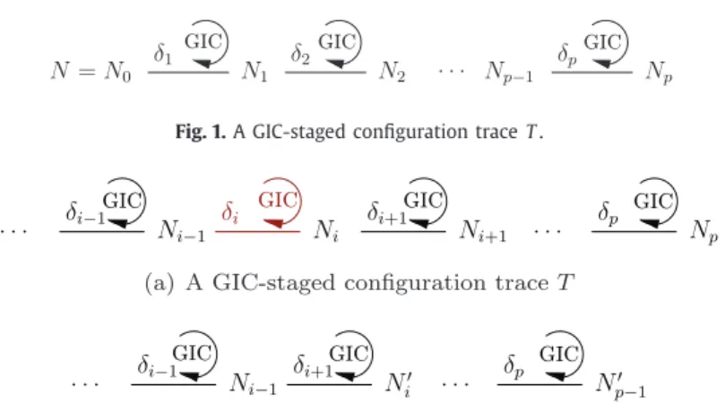
Fig. 1. A GIC-staged configuration trace T .
Fig. 2. Restoring GIC-staged configuration traces.
and thecurrent tablearesufficientbythemselvestoprovethat allvaluesareGIC).This roughanalysisoftimecomplexity suggeststhat GIC3andGIC4mightbethebestoptions.
Observethat whenGICismaintainedduringsearch,one canalwaysenforcetheweaker(and cheaper)consistency GAC before GIC.Thisistheapproachwesystematicallyfollowwhenmaintaining GICduringsearch(withany oftheintroduced GIC algorithms).
5. AnalgorithmforrestoringGIC
Inthissection,weaddresstheissueofrestoringGICaftertheuserdecidestodiscardarbitrarilyadecisionthathas been takenduringaconfigurationprocessbasedonGIC.So,thecontextisaCNN thatisgiveninitially,asequenceof p decisions
1= hδ1,δ2,. . . ,δpitakenon N (inthat order)bytheuser,andGICmaintainedon N.
Moreformally,aconfigurationtrace T onaCNN fromasequenceofdecisionshδ1,. . . ,δpi isrepresentedbyasequence
of CNs hN1,. . . ,Npi such that Ni is the CN obtained from Ni−1 (starting with N0=N) after taking the decision δi and
running somepropagationalgorithm.For eachdecision δi, itiseasytoidentifytheset deleted(δi)ofvaluesdeleteddue
to thecombinedeffectofδi andconstraintpropagation: wehavedeleted(δi)= values(Ni−1)\ values(Ni).Thesesets
areusefulforbacktracking,forexamplewiththeso-calledtrailing mechanism(seee.g.,[21]).
Withoutlossofgenerality,weassume that N is(orhas beenmade)initiallyGIC.AconfigurationtraceT= hN1,. . . ,Npi
on N from hδ1,. . . ,δpi isGIC-staged iff Ni=G I C(Ni−1|δi), ∀i∈1..p. Inother words, a GIC-staged configurationtrace isa trace suchthat GICismaintainedateach step.Anillustration isgivenbyFig. 1, whereeachedgerepresents theactionof takingadecisionδi and enforcingGIC:wehave N1=G I C(N0|δ1), N2=G I C(N1|δ2),. . ., Np=G I C(Np−1|δp).
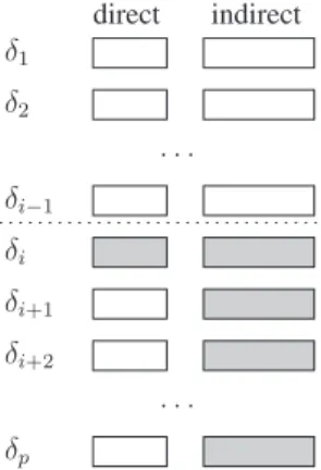
In our work, we are interested in GIC-staged configuration traces, and our objective is to be able to rebuild GIC-staged configuration traces after discarding arbitrarily any taken decision(s). Note that it has the flavor of dynamic backtracking [22], but in the context of the very strong consistency GIC. An illustration of a GIC-staged configuration trace, T = hN1,. . . ,Ni−1,Ni,Ni+1,. . . ,Npi, is given by Fig. 2(a): we have, N1=GIC(N0|δ1), . . ., Ni−1 =GIC(Ni−2|δi−1),
Ni=GIC(Ni−1|δi),Ni+1=GIC(Ni|δi+1),. . ., Np=GIC(Np−1|δp).Ifeverthedecisionδi isdiscardedbytheuser,thenwewant to computeanewGIC-stagedconfigurationtrace, T′= hN1,. . . ,Ni−1,N′i,. . . ,N′p−1i,asinFig. 2(b), where N1=GIC(N0|δ1), . . ., Ni−1=GIC(Ni−2|δi−1), N′i=GIC(Ni−1|δi+1), . . ., N′p−1=GIC(N′p−2|δp). Hence, weneedto compute p−i newCNs: N′i,
. . ., N′
p−1, but as observed earlier, it suffices to identifythe (new) sets of deleted values at levels i, . . ., p−1. Later, in Algorithm 9,thiswillbetheroleofthedatastructureKnw.
Reclassifying adeletedvalueoftraceT means findingthelevelatwhichthisvalue mustbedeletedinthenewtrace T′, or proving that it isno longer deleted. It isworthwhile to analyze which values mustbe reclassified when a decision is discarded and anewGIC-stagedconfigurationtraceisaimedtobecomputed.First, ateachlevel, i.e.after eachdecision δ, we can distinguish between the values that are directlyremoved by δ and those that are removed by propagating these initial directdeletionsthrough theCN.Forexample, ifx isavariablesuchthat dom(x)= {a,b,c} and δ correspondstothe variable assignment x=a, thenthevalues directlyremoved byδ are{b,c}. All other valuesremoved whileenforcing GIC aftertakingδaresaidtobeindirectlyremoved byδ.Thedifferentsetsofvaluesthatareremovedeitherdirectlyorindirectly inaGIC-stagedconfigurationtracearedepictedinFig. 3.
Inthefollowing,forthesakeofsimplicity,weassumethatalldecisionscorrespondtovariableassignments.Interestingly, oncethedecisionδiisdiscarded,computingthenewGIC-stagedconfigurationtraceT′onlyrequirestoreclassifythedeleted
valuesthat belongtothegrey-coloredregionsofFig. 3.Theproofisasfollows:
1. nothing changes for levels strictly less than i; in other words, for any integer j such that 0< j<i, deleted(δj)
Fig. 3. The deleted values that need to be reclassified, when the decisionδiis retracted, are those in grey-colored regions.
2. any value (x,a) directly removed by adecision δj with j>i will necessarily beagain removed directlyby δj in the
newtrace;in otherwords, (x,a) remainsindeleted(δj).2 Indeed,therelaxation(retracted decision)doesnotallow
ustoremove(x,a) beforetakingδj inthenewtrace.
All valuesthat mustbe reclassifiedare putina datastructurecalled Unk and transferredprogressively, whilerunning thealgorithmwepropose,toadatastructurecalledKnwthat weintroducelater.
To restore GIC, Function restoreAfterDeleting(), presented inAlgorithm 9, mustbe called.When thisfunctionis called for, itisforaGIC-staged configurationtrace T= hN1,. . . ,NpionaCNN fromasequenceofdecisions1= hδ1,. . . ,δpi.For
simplicity and because we assume that ateach decision level, i.e. for eachdecision δ, we knowdeleted(δ), only Np is specifiedasaparameter(aswellasthedecisionδi tobediscarded).Generalstatements usefulfordescribingouralgorithm
are:
• take(δ) : the decision δ is added at the endof the current sequence of decisions (push operation) and deleted(δ) initiallycontainsthevaluesofdom(var(δ)) thatarenotcompatiblewithδ (directdeletions).
• backtrack() :thelasttakendecisionδ isremovedfromthecurrentsequenceofdecisions(pop operation)andvaluesin deleted(δ)arerestoredindomains.
Thedatastructuresusedbyourfunctionarethefollowing:
• 1replay isthesequencehδi+1,δi+2,. . . ,δpi ofdecisionstobereplayed,once δi isdiscarded.
• Knwisanarrayofsize p−i+1,indexedfromi to p,ofsetsofvalues.Thisisacentraldatastructureinouralgorithm, allowingusto rebuildtheGIC-staged configurationtrace T′.Once thecomputation ofthisarray isfinished, allvalues arereclassified.If(x,a)∈ Knw[h]withi≤h<p,thismeansthat (x,a) mustbedeletedatlevelh,butif(x,a)∈ Knw[p], thismeansthat (x,a)willnomorebedeletedinthenewtrace(becauseweonlykept p−1 decisions).
• Unkisamapthatassociatesanintegerintervalhmin..hmax,calledclassificationinterval,witheachkeyoftheform(x,a). Themeaningofanentry((x,a),hmin..hmax) ofUnkisthat thevalue (x,a) mustbereclassified atalevel rangingfrom hmintohmax.Duringtheexecutionofthealgorithm,theclassificationintervalofeveryentryisrefineduntil theprecise
deletionlevel isknown,i.e.until hmin=hmax, inwhichcasetheentry isdeletedand transferredtothestructureKnw, described above. Notice that when the classification interval associated with a value ends up at p..p, this actually meansthatthevalueisno moredeletedbyGIC.As anymap,Unksupportsthefollowingoperations:
– Unk.clear()emptiesthemap,
– Unk.containsKey((x,a))indicatewhetherornotthereisanentryforkey(x,a), – Unk.get((x,a))returnstheintegerintervalassociatedwithkey(x,a),
– Unk.put((x,a),hmin..hmax)storesthepair((x,a),hmin..hmax) possiblyreplacingany previousentry withkey (x,a),
– Unk.size()returnsthenumberofentriesinthemap, – Unk.delete((x,a))deletestheentry withkey(x,a).
Before presenting function restoreAfterDeleting() in detail, we describe the two primitive functions increaseMin and decreaseMax thatwillbeusedtoupdatetheclassificationintervalofakey(x,a)inUnkandmovesuchakeytoKnwwhen needed. Function increaseMin((x,a),h) (Algorithm 7) first retrieves the interval for key (x,a) in Unk (line 1). If the new lower bound h reduces theinterval to a singleton, the key (x,a) is transferred from Unk to Knw with theright deletion level (lines2–4).Otherwise,ifthelowerboundchanged,theintervalisupdated(lines5–6).Function decreaseMax((x,a),h)
2 Strictlyspeaking,thevalue(x,a)isdeletedbyδ
Algorithm 7: increaseMin((x,a) :value,h : integer). 1 hmin..hmax← Unk.get((x,a))
2 if h=hmaxthen 3 Unk.delete((x,a)) 4 Knw[h]← Knw[h]∪ {(x,a)} 5 elseif h>hminthen
6 Unk.put((x,a),h..hmax)
Algorithm 8: decreaseMax((x,a) :value,h : integer). 1 hmin..hmax← Unk.get((x,a))
2 if h=hminthen 3 Unk.delete((x,a)) 4 Knw[h]← Knw[h]∪ {(x,a)} 5 elseif h<hmaxthen
6 Unk.put((x,a),hmin..h)
Algorithm 9: restoreAfterDeleting(Np:CN,δi :decision).
Input: Np isthelastCNofthecurrentGIC-stagedconfigurationtraceT= hN1,. . . ,Ni,. . . ,Npifromhδ1,. . . ,δi,. . . ,δpi.
Input:δi isthedecisiontodiscard.
Result: AnewGIC-stagedtraceT′fromhδ1,. . . ,δ
i−1,δi+1,. . . ,δpi // Initialization of structures 1 1replay← hδi+1,δi+2,. . . ,δpi 2 Unk.clear() 3 foreach j from i to p do 4 Knw[j]← ∅
// Deleted values of the current trace T to (re)classify 5 foreach j from p downto i+1 do
6 foreach(x,a)∈ deleted(δj)do 7 if x=var(δj)then
8 Knw[j−1]← Knw[j−1]∪ {(x,a)} // directly removed
9 else
10 Unk.put((x,a),j−1..p) // value to reclassify
11 backtrack()
12 foreach(x,a)∈ deleted(δi)do 13 Unk.put((x,a),i..p) 14 backtrack()
// Refining classification intervals 15 refineIntervals(Unk,Knw,1replay)
// Finalizing classification 16 whileUnk.size 6=0 do
17 foreach((x,a),hmin..hmax)∈ Unkdo 18 pickavalues in[hmin..hmax−1]
19 I←searchSolutionFor(N|{δ j∈1replay|j≤s+1}∪{x=a}) 20 if I=nil then 21 decreaseMax((x,a),s) 22 else 23 foreach(y,b)∈I do 24 ifUnk.containsKey((y,b))then 25 increaseMin((y,b),s+1)
// Building the new trace T′
26 foreachδj∈ 1replay(withj fromi+1 top) do 27 take(δj)
28 foreach(x,a)∈ Knw[j−1]do
29 remove(x,a)
(Algorithm 8)behavesthesameway:itretrievestheintervalfor(x,a),checkswhetherthenewupperboundh reducesthe interval toasingleton, anddependingontheanswertransfers(x,a) toKnworupdatestheupperbound.
Function restoreAfterDeleting()worksasfollows.Lines1–4initializethestructures: thedecisionstobereplayedareput in 1replay, and structuresUnk and Knw areemptied because deletedvalues to bereclassified arenot known yet,and so,
Algorithm 10: refineIntervals(Unk,Knw,1replay). Input:Unk,Knw:datastructures.
Input:1replay:sequenceofdecisions.
Result: UpdatedclassificationintervalsinUnkandpossiblynewkeysinKnw.
1 foreachδj∈ 1replay(withj fromi+1 top) do 2 take(δj)
3 enforceGAC()
4 foreach j from p downto i+1 do
5 foreach(x,a)∈ deleted(δj)do 6 ifUnk.containsKey((x,a))then
7 decreaseMax((x,a),j−1)
8 backtrack()
no classification has been performed yet.Line 5–14 handle all values that have been deleted from level i in the current trace T . Alllevels, from p down toi,areiteratedover,bysystematically backtracking(lines11and 14).The newstatusof any deletedvalue(x,a)atalevel j>i iseitherknown(line 8),becauseofadirectdeletion,orunknown(line 10).Forthe former case, thetestat line7issufficientbecause weonly consider variableassignments.For thelattercase,the interval
j−1..p boundsthedifferent possibilities(thevaluecannot bedeletedatalevel lessthan j−1 andpossibly canremain valid at the end of the new trace). For level i (lines 12–13), as shown in Fig. 3, all deleted values must be reclassified. Line 15 attempts to refine the classification intervals of values byapplying apolynomial process, such assimulating GIC by anefficient local consistency technique.We show laterhow to useGAC for refining theintervals. Lines 16–25 finalize classification. Foreachunclassified value (x,a), wehavean intervaloftheform hmin..hmax.Given (x,a),we selectavalue
(level) s thatwillbeusedto decreasethesize oftheintervalof(x,a);forourexperimentation,weshall selecthmax−1.In
line 19,we call searchSolutionFor inthenetwork where weforce alldecisionsfrom δi+1 to δs+1 (that correspondto new
levels i tos)plus x=a. Thepurposeofthiscallto searchSolutionFor isto checkifthereexistsasolutionfor(x,a) atlevel
s.If thisisnotthecase,wecandecreasetheupperboundoftheintervalto s (since,weknowthatGICisenoughtoprune this valueat level s).Otherwise, we canincrease thelower bound ofall unclassifiedvalues that are present inthefound solution I (see Lines 23–25). This includes of course (x,a). Lines 26–29 build the new GIC-staged configuration trace T′ fromdatainKnw.
Reclassifyingvalues maybeexpensivebecause forproving GIC ofavalue wehave torun acompletesearchprocedure (see line19), and possibly several times. One idea is to usea cheap process, such as applying GAC, asan approximation of GICinapreliminary stage.For example,suppose that ((x,a),10..14)ispresent in Unkand that MACremoves (x,a) at level 10. We can then deduce that (x,a) isGIC-inconsistent at level 10, and consequently directly classify (x,a) in T′. If MAC removes(x,a) onlyatlevel 12,thenwecanreplace((x,a),10..14) by((x,a),10..12) inUnk.Tosummarize,running MAC on decisions of1replay allowsusto refine theclassificationintervals atavery moderateprice. Thiswhat isdoneby thefunctionrefineIntervals(Unk,Knw,1replay) inAlgorithm 10.
Inlines 1–3,GACismaintainedafter eachdecisiontaken insequencefrom 1replay. Then,inlines 4–7,weprocesseach level insequencefrombottomtotop.If (x,a)has beendeleted(atlevel j−1)byGACafter decisionδj,weknowthat GIC
will prune(x,a) atlevel j−1 atthevery last. Hence,weupdate theintervalof (x,a) accordingly. Afterhaving processed allvalues ofalevel,we havetocall the backtrack functiontorestoredomainsinthestate theywerebeforeapplying GAC (line 8).
Wehave theguaranteethat restoreAfterDeleting performsasif GIChad been maintainedon N from hδ1,. . . ,δi−1,δi+1,
. . . ,δpi.Theproofisbasedon theinvariantpropertythat Unkissound,thatis,thelevelofdeletionofany(x,a)presentin
Unk iscontainedintheintervalstoredinUnk.
Lemma1.IfUnkissoundbeforeacallto refineIntervals,thenitremainssoundaftertheexecutionof refineIntervalsasdescribedin
Algorithm 10.
Proof. Theintervalof(x,a) inUnkismodifiedinline7only ifGAChas removed(x,a)afterdecision δj hasbeen applied.
ByenforcingGICinsteadofGAC,itisobviousthat(x,a)cannotberemovedlater.Thus,thelastlevel atwhich(x,a) canbe removedis j−1 becauseδj isthe(j−1)thdecision. ✷
Theorem 7.Let hN1,. . . ,Npi be a GIC-stagedconfigurationtraceona CN N from asequence ofdecisions hδ1,. . . ,δpi.Calling
restoreAfterDeleting(Np,δi)buildstheGIC-stagedconfigurationtraceonN fromhδ1,. . . ,δi−1,δi+1,. . . ,δpi.
Proof. Lines11 and 14ensurethat, afterline14, allvaluesremoved inlevels i to p have been restoredand puteitherin Knw orinUnk.Theywillthus allbeprocessedtofindtheirrightlevelofdeletion.
Wefirstprovethatbeforeline26,allvaluesareputinKnwattheirrightlevelofdeletion.Afterlines1–14areexecuted, all values in Knw have been put in it at line 8. They have been put at their right level because they cannot be higher
Table 1
FeaturesofsixRenaultconfigurationinstances.
n d e r t D T Souffleuse 32 12 35 3 55 145 350 Megane 99 42 113 10 48,721 396 194,838 Master 158 324 195 12 26,911 732 183,701 Small 139 16 147 8 222 340 3,044 Medium 148 20 174 10 2,718 424 9,532 Big 268 324 332 12 26,881 1,273 225,989
(relaxation)andtheyarenecessarilyremoved(line7tellsustheybelongtotheinstantiatedvariable).Afterlines1–14,Unk is soundbecause it storesthe largest possible interval forevery non-reclassified value. After line 14, intervalsare refined in lines 15,21, and 25. ByLemma 1, Unkremains soundafter line15.In line21, thehmax of (x,a) isdecreased correctly
because there wereno solutions containing (x,a) atlevel s.In line25, it isalso obviouslycorrect to increasethehmin of
(y,b) tos+1 aswefoundasolution atlevel s.By constructionoffunctions increaseMin and decreaseMax,weknowthat after line25,Knw containsonlycorrect levelsofdeletion.
Wethenprovethattheloopinlines16–25terminates.Whenweentertheloopinline16,Unkonlycontainsvalueswith a non-singleton interval. By constructionof increaseMin and decreaseMax, any value withan interval shrunk tosingleton is moved to Knw. Thus, line 17 can only selectvalues with non-singleton intervals, and the way s is selected in line 18 ensures that any iterationof theloopofline17 strictly decreasesthe sizeofat leastone interval inUnk. As allintervals have finitesizeandasUnkcontainsafinitenumberofvalues,theloopofline16 terminates.
The factthat after line25allvalues areputinKnw attheir rightlevel ofdeletion and thefactthat thealgorithm will eventuallyreachline26guaranteesthatlines 26–29buildaGIC-stagedconfigurationtrace. ✷
The algorithm restoreAfterDeleting is obviouslyexponential intime as it solvesan NP-hardproblem (see Theorem 4). Nevertheless,wecananalyzethenumberoftimesitcallstheNP-hardoracle searchSolutionFor.
Theorem8(Complexity).LethN1,. . . ,NpibeaGIC-stagedconfigurationtraceonaCNN fromasequenceofdecisionshδ1,. . . ,δpi. Thenumberoftimes restoreAfterDeleting(Np,δi)calls searchSolutionForisinO(nd·log2(p−i)).
Proof. Eachtime searchSolutionFor is calledinline19, theinterval of(x,a)isshrunk eitherto[hmin,s] orto[s+1,hmax],
depending on whetherline21 orline25isexecuted. Hence,if s is selectedina dichotomicway(that is, s= ⌊hmin+hmax
2 ⌋),
each call to searchSolutionFor leads to an interval of size at most ⌈hmax−hmin+1
2 ⌉. Unk contains at most nd values and
intervalscannotbelargerthan p−i+1.Asaresult,thenumberoftimes restoreAfterDeleting cancall searchSolutionFor is in O(nd·log2(p−i)). ✷
6. Experiments
Inordertoshowthepracticalinterestofourapproach,wehaveperformedseveralexperimentsmainlyusingacomputer withprocessorsIntel(R)Core(TM)i7-2820QMCPU2.30 GHz;however,forGICrestoration,weusedaclusterofXeon3.0 GHz processors with13 GB ofRAM. Ourmainpurpose was to determine whethermaintaining/restoringGIC is aviable option for configuration-like probleminstances (and forinteractive puzzle creation), aswellas tocompare the relativeefficiency ofthefourGICalgorithmsdescribed inSection 4.
In Table 1, weshow relevant features of car configurationinstances, generated withthe help of ourindustrial partner Renault.Foreachofthesixinstancescurrentlyavailable,3 weindicate
• thenumberofvariables(n), • thesizeofthegreatestdomain(d), • thenumberofconstraints (e), • thegreatestconstraintarity(r), • thesizeofthegreatesttable(t),
• thetotalnumberofvalues(D=Px∈vars(N)|dom(x)|), • andthetotal numberoftuples(T =Pc∈cons(N)|rel(c)|).
Table 2
CPUtime(inseconds)toestablishGIConRenaultconfigurationinstances,andtomaintainit(average over100randomgreedyexecutions).
Establishing GIC with Maintaining GIC with
GIC1 GIC2 GIC3 GIC4 GIC1 GIC2 GIC3 GIC4
Souffleuse 0.02 0.01 0.01 0.01 0.13 0.07 0.02 0.02 Megane 2.94 0.71 0.72 0.71 4.26 1.18 0.05 0.04 Master 2.45 1.35 1.33 1.33 9.81 3.57 0.07 0.06 Small 0.14 0.02 0.03 0.03 0.32 0.05 0.01 0.01 Medium 0.26 0.04 0.05 0.04 0.35 0.04 0.01 0.01 Big 4.19 1.16 1.10 1.10 12.6 2.60 0.05 0.05 Table 3
NumberofconflictsencounteredwhenrunningnFC2andMAC(sumover100randomexecutions).
Souffleuse Megane Master Small Medium Big
nFC2 252,605 313,910 time-out 3,728 7,824 time-out
MAC 0 7 5 0 3 3
Table 4
CPUtime(inseconds)toestablishGIConsomeCrosswordsinstances,andtomaintainitonaverage over100randomgreedyexecutions.
Establishing GIC with Maintaining GIC with
GIC1 GIC2 GIC3 GIC4 GIC1 GIC2 GIC3 GIC4
ogd-vg5-5 2.25 0.67 0.67 0.67 2.34 0.79 0.73 0.70
ogd-vg5-6 6.40 2.18 2.19 2.19 7.42 2.82 2.58 2.48
ogd-vg5-7 25.8 9.91 9.87 9.84 33.4 15.2 14.3 13.8
6.1. Establishing/maintainingGIC
TheleftpartofTable 2presentstheCPUtimerequiredtoestablishGIConthesixRenaultconfigurationinstances.Clearly GIC1isoutperformedbythethreeotheralgorithms,whichhavehererathersimilarefficiency.TherightpartofTable 2aims atsimulatingthebehaviorofaconfigurationsoftwareuserwhomakesthevariablechoicesandvalueselections.Itpresents the CPU timerequired to maintain GIC along a completebranch built by performing random variable assignmentsdown to a leaf. (Random variable assignment simulates the user, who chooses the variables and the values according to her preference.)Specifically,variablesandvaluesarerandomlyselectedinturn,andaftereachassignment,GICissystematically enforcedtomaintainthisproperty.Ofcourse,noconflict(dead-end)canoccuralongthebranchdue tothestrengthofGIC, which iswhyweusethetermofgreedyexecutions.CPUtimesaregiven onaveragefor 100executions(differentrandom orderings). When establishing GIC, any call to searchSolutionFor is performed with the help of the algorithm MAC (table constraints being filteredwiththetechnique calledSimple TabularReduction[19,20,23]). For allinstances,GIC3 and GIC4 aremaintainedveryfast,whereason thebiggestinstances,GIC2requiresafewsecondsandGIC1aroundtenseconds.
OnegreatadvantageofGICisthat itguaranteesthataconflictcanneveroccurduringaconfigurationsession.However, one may wonder whether the risk of failure(s) is reallyimportant in user-driven searches that use a weaker consistency such asGAC or apartial form ofit (ForwardChecking). Table 3 showsthe numberof conflicts (sum over 100executions usingrandomorderings)encounteredwhenfollowingaMAC oranFC2[24]strategy.Thenumberofconflictsituationscan bevery largewith nFC2(fortwo instances,weeven reporttheimpossibility offindingasolution within10minutes with some random orderings). For MAC, thenumberoffailures israthersmall but the risk isnotnull (forexample, therisk is equalto7%for megane).
The encouraging results obtained on Renaultconfiguration instancesled usto test other problems,in particularto get a betterpicture oftherelativeefficiencyofthe variousGICalgorithms. For example,on classical Crosswordinstances(see
Table 4), GIC1is once again clearly outperformed while thethree other algorithms are quite close, where there is still a small benefitofusingGIC4.
It is worthwhile to note that GIC isa nice property that can be usefulwhen puzzles, where hints are specified, have to becreated.Typically, one looks forpuzzles where only onesolution exists. Onewayof buildingsuchpuzzles is toadd hints insequence, whilemaintainingGIC, until alldomainsbecomesingleton.For example, thisisapossibleapproach for constructing SudokuandMagic Squaregrids,withtheadvantage thattheusercanchoosefreelythepositionofthehints.4 On the left partof Table 5, wereport thetime to enforceGIC on empty Sudoku gridsof size 9×9 and 16×16, and on emptyMagic squaresofsize4×4 and 5×5.On therightpart wereporttheaverage timerequiredto maintainGICuntil
Table 5
CPUtime(inseconds)toestablishGIConPuzzleinstances,andtomaintainitonaverageover100random greedyexecutionsuntilauniquesolutionisfound.
Establishing GIC with Maintaining GIC with
GIC1 GIC2 GIC3 GIC4 GIC1 GIC2 GIC3 GIC4
sud-9×9 1.58 0.32 0.32 0.31 15.3 2.71 2.10 1.74
sud-16×16 6.04 0.51 0.50 0.50 246 25.5 26.5 18.9
magic-4×4 0.96 0.26 0.28 0.28 1.63 0.69 0.71 0.71
magic-5×5 14.7 3.01 3.10 2.99 55.1 15.9 15.6 13.7
allvariablesbecomefixed(i.e.,withonlysingletondomains),meaningthatafterseveralhintshavebeenrandomlyselected and propagated, we have theguarantee of having a one-solutionpuzzle. GIC4is a clear winner,with for example, a 30% speedup overGIC2andGIC3on sudoku-16×16,and morethanoneorderofmagnitudeover GIC1.Overall,theresults we obtain show that maintainingGIC isapracticablesolution (at leastfor someproblems)astheaverage timebetweeneach decisionoftheuserissmallwithGIC4.
6.2. RestoringGIC
Inasecondsetofexperiments,wehavefocusedontheissueofrestoringGIC,asdevelopedinSection5.Wehavetested
Algorithm 9againstallRenaultcarconfigurationinstancesintroducedearlier.Foreachinstance,theprotocolwehaveused is the following. First, we have built a complete GIC-staged configuration trace T (branch), by randomly assigning each variableinturn(andsubsequentlymaintainingGIC).Then,wehavediscardedarbitrarilyadecisionused forT , andapplied our algorithm that restores GIC. Actually, we have successively collected information about GIC restoration for decisions discarded at levels i ranging respectively from 0 (first decision taken) to 80.5 After decision 80, all these instances only contain singletondomains,andso, arecompletelysolved.Inotherwords, wehaveindependentlytestedGICrestorationon
T ,whenadecisionwasdiscardedatleveli=0,atlevel i=1,andsoonuntil level80.Theresultswepresent aregivenon averageover100randomcompleteGIC-stagedconfigurationtracesperlevel.Suchtracesarecomputedinitiallybyrandomly selectingdecisions.
Wehavebeeninterestedin:
• thetotalnumberofvalues(i.e.,thenumberofvaluesoverallvariabledomains),denotedby# values
• thenumberofunclassifiedvalueswhendiscardingadecision,atthepointbeforerefiningclassificationintervalsthrough MAC;thisisdenotedby“#? valuesbeforerefinement”
• thenumberofunclassifiedvalueswhendiscardingadecision,atthepointjust afterhavingrefinedclassification inter-valsthroughMAC;thisisdenotedby“#? valuesafterrefinement”
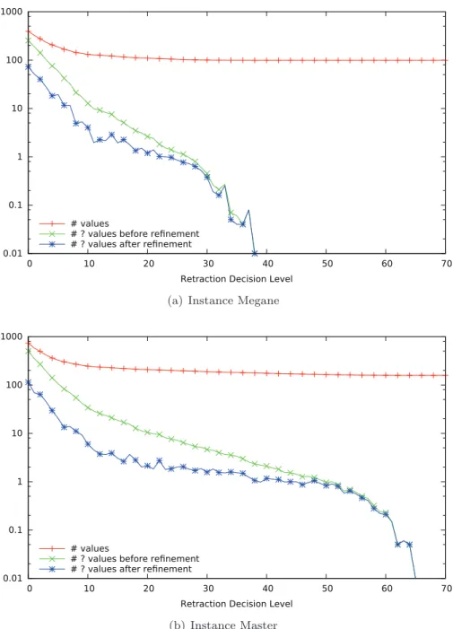
Wehave observedthesametrendwhen testingthe6configurationinstances:i) it isonly whentheretracted decision belongsto thefirstones takenbytheuserthat asubstantialcomputing effortisrequired, and ii) classificationrefinement byMACisvery useful.Figs. 4(a)and4(b)showresultsforthecarmodelsMegane(amid-sizeinstance)andMaster (alarge size instance).The x-axisindicatesthelevel atwhich thedecision(fromthecompleteGIC-staged configurationtrace)was discarded beforerestoringGIC.Forexample,whentheretractiondecisionlevelis8,wecanseeforMasterthat thenumber of unclassified values after MAC refinement is around10 (on average). The impactof classification refinementby MAC is clearlyvisible,asitcorrespondstothegapbetweenthetwobottomcurves.(Notethelogarithmicscaleforthe y-axis.)The two curvesonlymergewhentheaveragenumberofunclassifiedvaluesisaround 1.
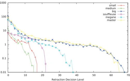
Itisalso interestingtoseehow many callstotheprocedure (oracle) searchSolutionFor arenecessarytoclassify the re-mainingunclassifiedvaluesafterrefiningintervalsthroughMAC.InSection5,wementionedthepossibilityofadichotomic approach(see Theorem 8).However,forconfigurationinstances,pickings=hmax−1 atline18ofAlgorithm 9isarelevant
choice because mostof thetime itallows usto prove directlythat the value isGIC-consistent. This iswhat wehave ob-served: theproportionofsuccessfulcalls(i.e.,ofcallsreturning asolution) isvery high.Besides,whenasolution isfound, multidirectionalitycanbeusedtorefineclassificationintervalsofothervalues(lines23–25inAlgorithm 9).Fig. 5showsthe average numberofcallsto searchSolutionFor foreachinstanceand eachretractiondecisionlevel. Forthelargest instances, intheworst-case (level0),thenumberofcallsisaround100.Atlevel8,lessthan 10callsarerequired.Table 6showsthe averagenumberofunclassifiedvaluesafterGACrefinement(#?values)andtheaveragenumberofcallsto searchSolution-For (# calls), computedoverallretractiondecision levels.Thenumberofcallstotheoracle isnevermorethan75% ofthe numberofunclassifiedvalues.
Table 7gives theCPUtimerequiredto restoreGIC. Theworst-case maximumtime is1.5secondsfor megane,butnote this is only 0.2 second on average. This confirms that our approachcan perfectly beused in aninteractive configuration context.
Fig. 4. Restoring GIC at different decision levels. Average values over 100 executions.
Table 6
AveragenumberofunclassifiedvaluesafterGACrefinement(#?values)andaveragenumber ofcallsto searchSolutionFor (#calls)forRenaultcarconfigurationinstances.
Souffleuse Megane Master Small Medium Big
# ? values 3.23 3.68 5.95 2.05 2.27 9.67
# calls 2.22 2.92 4.92 0.40 0.49 4.44
Finally, Table 8 shows how the algorithm we propose for restoring GIC after discarding a decision δi (referred to as
optimizedGICrestoration)behaveswithrespecttoasimplealgorithm(referredtoasnaiveGICrestoration)thatjusterases all decisionsfrom δi to thelast before replaying allofthemexcept thediscarded decision δi,while maintainingGIC with
GIC4.The resultsaregiven onaveragefor100randomGIC-staged configurationtraces,withGICrestorationtriggeredafter 80 decisions havebeen taken (32for souffleuse) and the firstof these decisionshas been discarded. Note that discarding thefirst decisionisthemostadversecase(i.e.,requiring themostcomputing effort),whichisthereasonfor studyingthis particularcase.Weobservethatduringthisprocess,thenumberofcallstotheoracle searchSolutionFor isverylimitedwhen ouroptimizedalgorithmisused.Ouralgorithmisbetween2and5timesfasterthanthenaiveone.Ontheseinstances,our algorithmneverrequiresmorethan1second.
Fig. 5. Restoring GIC at different decision levels. Number of calls to the procedure (oracle) searchSolutionFor. Average over 100 executions.
Table 7
Minimum,maximumandaverageCPUtimesinsecond(s) to restore GIC, after discarding any decision (in range 0..80).Valuesarecomputedover100randomtraces.
min avg max
Souffleuse 0 0.002 0.006 Megane 0 0.247 1.440 Master 0.001 0.225 0.722 Small 0 0.006 0.013 Medium 0 0.006 0.011 Big 0.001 0.212 0.855 Table 8
Minimum, maximumandaverageCPUtimesinmillisecond(s) torestore GIC,after dis-cardingthefirstdecisionof asequencecomposedof80decisions.Theaveragenumber ofcallstotheprocedure(oracle) searchSolutionFor isalsoindicated.Valuesarecomputed over100randomtraces.
Naive GIC restoration Optimized GIC restoration
min avg max # calls min avg max # calls
Souffleuse 1 5.1 20 157.1 0 0.1 5 6.9 Megane 35 507 1,387 223.4 13 145 632 61.2 Master 27 1,033 2,860 582.2 8 202 924 89.2 Small 1 8.9 93 53.7 0 2.9 18 7.2 Medium 2 12.6 39 42.1 1 6.3 24 14.3 Big 39 877 2,251 514.8 6 247 988 115.1 7. Conclusion
Wehaveanalyzedtheproblemsthat ariseinapplications thatrequiretheinteractiveresolutionofaconstraintproblem by ahumanuser. The centralnotion isglobal inverse consistencyof thenetwork because itensures that theperson who interactively solves the problem is not given the choice to select values that do not lead to solutions. We have shown that deciding, computing, or restoring global inverse consistency, and other related problems are all NP-hard. We have proposed several algorithms for enforcing/maintaining/restoring global inverse consistency and we have shown that the best version is efficient enough tobe used in aninteractive setting on several configurationand design problems.This is a great advantage compared to existing techniques usually used in configurators. As opposed to techniques maintaining arc consistency, ouralgorithmsgivean exactpictureofthevalues remainingfeasible.As opposed tocompiling offline the problemasamulti-valueddecisiondiagram,ouralgorithmscandealwithconstraintnetworks thatchange over time(e.g., anextranon-unaryconstraintposted byacustomerwhodoesnotwanttobuyacar withmorethan 100,000milesexcept if itisaVolvo). Onedirectperspective ofthisworkisto trycomputing diverse solutionswhenenforcingGIC. Thisshould allow, onaverage,toreducethenumberofsearchruns.Techniquessuchasthosedevelopedin[25]mightbeuseful.