Effective surface and boundary conditions for heterogeneous surfaces with mixed boundary conditions

O

pen

A

rchive

T

OULOUSE

A

rchive

O

uverte (

OATAO

)

OATAO is an open access repository that collects the work of Toulouse researchers and

makes it freely available over the web where possible.

This is an author-deposited version published in :

http://oatao.univ-toulouse.fr/

Eprints ID : 14533

To link to this article : DOI :

10.1016/j.jcp.2015.10.050

URL :

http://dx.doi.org/10.1016/j.jcp.2015.10.050

To cite this version : Guo, Jianwei and Veran-Tissoires, Stéphanie and

Quintard, Michel Effective surface and boundary conditions for

heterogeneous surfaces with mixed boundary conditions. (2016)

Journal of Computational Physics, vol. 305. pp. 942-963. ISSN

0021-9991

Any correspondance concerning this service should be sent to the repository

administrator:

staff-oatao@listes-diff.inp-toulouse.fr

Effective

surface

and

boundary

conditions

for

heterogeneous

surfaces

with

mixed

boundary

conditions

Jianwei Guo

a

,

Stéphanie Veran-Tissoires

a

,

b

,

∗

_,

_{Michel Quintard}

a

,

c a_{UniversitédeToulouse,INPT,UPS,IMFT(InstitutdeMécaniquedesFluidesdeToulouse),31400Toulouse,France} b_{DepartmentofCivilandEnvironmentalEngineering,TuftsUniversity,Medford,MA02155,UnitedStates} c_{CNRS,IMFT,31400Toulouse,France}

a

b

s

t

r

a

c

t

Keywords: Heterogeneoussurface Multi-domaindecomposition Closureproblems Effectivesurface

Effectiveboundaryconditions

To dealwith multi-scaleproblems involvingtransport fromaheterogeneous and rough

surface characterized by a mixed boundary condition, an effective surface theory is

developed, which replacesthe original surface by a homogeneousand smooth surface

withspecificboundaryconditions.Atypicalexamplecorrespondstoalaminarflowovera

solublesaltmediumwhichcontainsinsolublematerial.Todeveloptheconceptofeffective

surface, amulti-domain decompositionapproach isapplied. Inthisframework, velocity

andconcentrationatmicro-scaleareestimatedwithanasymptoticexpansionofdeviation

termswithrespecttomacro-scalevelocityandconcentrationfields.Closureproblemsfor

the deviations are obtained and used to define the effective surfaceposition and the

relatedboundaryconditions.The evolution ofsomeeffective propertiesand the impact

of surface geometry, Péclet, Schmidt and Damköhler numbers are investigated. Finally,

comparisonsaremadebetweenthenumericalresultsobtainedwiththeeffectivemodels

andthosefromdirectnumericalsimulationswiththeoriginalroughsurface,fortwokinds

ofconfigurations.

1. Introduction

Transportphenomenatakingplaceoverheterogeneous andrough surfacescan befound inawide rangeofprocesses,

suchasdissolution,dryingorablationtociteafew.Thesurfacecharacteristiclength-scale(linkedtotheheterogeneities)is

generallymuchsmallerthanthescaleoftheglobalmechanism.Inthesecircumstances,directnumericalsimulations(DNSs)

becomedifficulttoachieveinpracticalapplications.Indeed,DNSsareonlypossiblewhenthetwolength-scaleshavemore

orlessthesameorderofmagnitude.Toovercomethisdifficulty,atraditionalwayofsolvingsuchproblemsistoincorporate

themicro-scalebehaviorsintoaboundaryconditionoverasmooth,“homogenized”oreffectivesurface.

In[1–3],domaindecompositionandmulti-scaleasymptoticanalysiswerefirstintroducedtodevelopaneffectivesurface

andthe associatedboundaryconditionsfortheflowover aroughsolid–liquid surface.Later,theeffectivesurface concept

wasusedtodescribeablationprocessesinaerospace[30]andnuclearsafety[15]contexts.Differentfromtheseworkswhich

employedasymptoticmethod,Woodetal.[33]obtainedaspatiallysmoothedjumpconditionfortheoriginallynon-uniform

surfacewithvolumeaveragingtechnique.Forsakeofsimplicity,mostofthepreviousstudiesignoredthegeometrychanges

*

Correspondingauthor.

E-mailaddress:stephanie.veran@u-bordeaux.fr(S. Veran-Tissoires).

Nomenclature

Roman symbols

A closure variable for the velocity

(dimension-less)

a closurevariablefortheconcentration

(dimen-sionless)

Aβγ surfaceareaofthesolublematerialin

Äi

m2

Aβσ surfaceareaoftheinsolublematerialin

Äi

. . . m2 B closurevariableforthevelocity . . . m

b closurevariablefortheconcentration . . . m

br roughnesswidth . . . m

c concentrationofthedissolvedspeciesdefined

in

Ä

. . . kg m−3

ceq thermodynamicequilibriumconcentrationof

thedissolvedspecies . . . kg m−3

ci concentrationofthedissolvedspeciesdefined

in

Äi

. . . kg m−3

˜

ci concentrationdeviationofthedissolved

speciesin

Äi

. . . kg m−3

c0 concentrationofthedissolvedspeciesdefined

in

Ä

0. . . kg m−3

D diffusioncoefficientofthedissolved

species . . . m2_s−1

Da Damköhlernumber(dimensionless)

Dav

eff effective Damköhler number at

6

effv

(dimen-sionless)

c

Da meanDamköhlernumberover surface

6

(di-mensionless)

e1 unitnormalvectorlinkedtox (dimensionless)

e2 unitnormalvectorlinkedtoy (dimensionless)

hr roughnessheight . . . m

k reactionratecoefficientat

6

. . . m s−1

kγ reactionratecoefficientat

6

βγ . . . m s−1

kσ reactionratecoefficientat

6

βσ . . . m s−1

k0

eff effectivereactionratecoefficientat

y

=

0 . . . m s−1

kc_eff effectivereactionratecoefficientat

6

c_eff. . . m s−1

k_effv effectivereactionratecoefficientat

6

_effv . . . m s−1

kw

eff effectivereactionratecoefficientat

y

=

w . . . m s−1

ˆ

kv _{surfaceaveragereactionratecoefficientat}

6

_effv . . . m s−1

l micro-scalecharacteristiclength . . . m

li widthof

Äi

. . . m

L macro-scalecharacteristiclength . . . m

m closurevariableforthepressure . . . Pa s m−1

nls unitnormalvectoron

6

pointingtowardsthe

solid(dimensionless)

n0,i unit normal vector on

6

0,i pointing towards

thewall(dimensionless)

p pressuredefinedin

Ä

. . . Pa

p0 pressuredefinedin

Ä

0. . . Pa

pi pressuredefinedin

Äi

. . . Pa

Pel micro-scalePécletnumber(dimensionless)

˜

pi pressuredeviationdefinedin

Äi

. . . Pa

Rel micro-scaleReynoldsnumber(dimensionless)

ReL macro-scaleReynoldsnumber(dimensionless)

s closurevariableforthepressure . . . Pa s

Sc micro-scaleSchmidtnumber(dimensionless)

u fluidvelocitydefinedin

Ä

. . . m s−1

ui fluidvelocitydefinedin

Äi

. . . m s−1

˜

ui fluidvelocitydeviationin

Äi

. . . m s−1 u0 fluidvelocitydefinedin

Ä

0. . . m s−1

U magnitudeofmacro-scalevelocity . . . m s−1

wc_x distancebetween

6

0 and

6

_effc . . . m

wv

x distancebetween

6

0 and

6

_effv . . . m

x abscissa . . . m

y ordinate . . . m

Greek symbols

β

subscriptreferringtothefluidphase

δ

effectivesurfaceposition . . . m

δc

positionof effectivesurface under

thermody-namicequilibrium(dimensionless)

δv

positionofeffectivesurface withno-slip

con-dition(dimensionless)

γ

subscriptreferringtosolublephase

σ

subscriptreferringtoinsolublephase

µ

fluiddynamicviscosity . . . Pa s

Ä

globaldomain

Ä

0 subdomainassociatedwithlengthscaleL

Äi

pseudo-periodicunitcell

ρ

fluiddensity . . . kg m−3

ρ

γ densityofsolublemedium . . . kg m−3

ρ

σ densityofinsolublematerial . . . kg m−3

6

roughsolid–liquidinterface

6

βγ interfacebetween

β

and

γ

phases

6

βσ interfacebetween

β

and

σ

phases

6

0 fictitioussurfaceseparating

Ä

0 and

Äi

6

0,i restrictionof

6

0in

Äi

6e

uppersurfaceof

Ä

6

_effc effective surface under thermodynamic

equi-librium

6

_effv effectivesurfacewithno-slipboundary

condi-tion

6l

lateralsurfaceof

Ä

andconsideredfixed boundaries. Ina few studies,thesegeometrychanges were takenintoconsideration. Vignolesetal.

[31]ranDNSsforablationofheterogeneousmedia.ArecentstudybyKumaretal.[21]alsoconsideredgeometrychanges

explicitlywhenupscalingthereactiveflowinadomainwithoscillatingboundaries,usingmatchedasymptoticexpansions.

Whiletherearesomesimilarities,oneshouldnotmixthesolid–liquidproblemwiththeproblemoffluidflowingovera

porousmediumdomain.Forthislattercase,oneseekstolinkamacro-scaledescriptionoftheflowintheporousmedium

(e.g.Darcy’slaw) to afree fluid flowdescription inthe channel(e.g., Navier–StokesorStokes equations).Different

effec-tiveboundaryconditionshavebeenproposed [6,10,26]forthe momentumbalanceequations.Formaldevelopmentsusing

homogenizationtechniques can be found in[10,17,18,20,26]. Different upscaling methods such asvolume averaging and

asymptoticexpansionshavebeenimplementedinordertoobtaineffectiveboundaryconditionsforvarioustransport

prob-lems[1,9,13,24,25,29,32].

In this work, the problem under consideration is mass andmomentum transfer in a laminar boundary layer over a

heterogeneousrough surface withmixedboundary conditions.Partof thesurface issubject to a Dirichletconditionora

reactive Neumannconditionwhilethe restissubject to a no-fluxNeumann condition.Such problemsarise, forinstance,

whendealingwithdissolutionprocesses,especiallyonlarge-scalecavityformationingeologicalstructures(solutionmining,

karstformations,etc.).Thegeometry,propagationandsome otheraspectsrelatedtoroughnessesgeneratedbydissolution

were studied experimentally andtheoretically in [7]. A similar mathematical problem appears when one considers the

dryingrateofaporoussurfacewithwetanddrypatches[27]orforatmosphere-scaleproblems[5].Takingthedevelopment

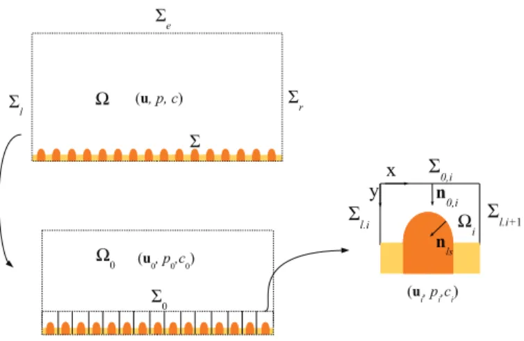
ofkarsticcavityforexample, itofteninvolves multi-scaleproblemsasschematically represented inFig. 1.It is generally

difficulttotake intoconsiderationthesmall-scaleheterogeneitiesoverthewall surfacewhileworkingatthecavityscale.

Therefore,theimplementedmodelsofsuchdissolutionproblemstakeinpracticetheformofaneffectivesurfacemodeling,

witha heuristic boundary condition. In generalone uses the Dirichletconditionas themacro-scale boundarycondition,

evenifheterogeneities(e.g.,insolublematerial)androughnessesarepresent. Thepositionoftheeffectivesurface itselfis

guidedbymeshingconsiderationwithoutan explicitlinktothephysicsoftheproblem.Thesequestionsareaddressedin

thispaperandamethodologyisproposedtobuildandpositiontheeffectivesurfacewithappropriateboundaryconditions.

Twolengthscalesareimportanttodescribethephenomenatakingplaceattherough surface:oneisthecharacteristic

lengthofthelarge-scalecavity,L,forinstancethedepthofthelarge-scaleboundarylayerdevelopingovertheroughsurface,

andthe otherone istheroughnesslengthscale l.As illustratedinFig. 1,a fluid

β

indomain

Ä

isflowingover arough,

heterogeneoussurface

6

,madeofasaltmedium

γ

andaninsolublematerial

σ

.Masstransportovertheroughsurfacein

contactwiththefluid canbemodeledbydifferentboundaryconditions.IncaseI, thesurfaceisassumedtobecomposed

bypatches underthermodynamic equilibrium(

6

βγ ), withsurroundingareaswithnoflux(

6

βσ ).IncaseII,theboundary

conditionat

6

βγ isreplacedbyareactiveone.Generally,thesurfacedissolutionrateofachemicalspeciescanbeexpressed

undertheform[16,22]:

Rdiss

=

ks

µ

1

−

cs ceq

¶

n (1)

wherecsisthetotalchemicalconcentrationatthesurface,ceq theequilibriumconcentrationwithrespecttothedissolving

speciesandks thesurfacereactionratecoefficient.

Thesteady-statemassandmomentumtransferproblemcanbedescribedasfollows

PbIin

Ä

ρ

(

u

· ∇)

u

−

µ

△

u

+ ∇

p

=

0 in

Ä

(2)

∇ ·

u

=

0 in

Ä

(3) u

· ∇

c

= ∇ · (

D

∇

c

)

in

Ä

(4) u

=

0 at

6

(5) (B.C. I) c

=

ceq at

6

βγ (6) or (B.C. II)

−

nls

·

D

∇

c

= −

kγceq

¡

1

−

_cc_eq

¢

at

6

βγ (7)

−

n

·

D

∇

c

=

0 at

6

e

, 6

βσ and

6

r (8) c

=

0 at

6

l (9) n

· (−

pI

+

µ

(∇

u

+ ∇

uT

)) =

0 at

6

eand

6

r (10) u

=

U0e1 at

6

l (11)

where,kγ isthereactionratecoefficientinm s−1,n isthenormalvectorpointingoutwardfromthestudieddomainat

6e

,

6l

,

6r

andthelatermentioned

6l

,i,andU0 denotesthemagnitudeoftheinletvelocity.Onehasn

=

nls at

6

βσ ,withnls

thenormalvectorof

6

pointingtowardsthesolidphase.B.C.IandB.C.IIrefertocaseIandcaseIIproblems,respectively.

Itisworthynoticingthatthenofluxconditionat

6e

andtheconstantvelocityconditionat

6l

arenotunique,whichcan

Fig. 1. Multi-scale description of the system. The dissolving medium is denoted asγ-phase and the non-dissolving part asσ-phase.

Fig. 2. Close-up view of the velocity field near the rough surface.

Eq. (7) hasa form similar to the rate laws proposed in [11,12,28] forlimestone andgypsum dissolution. First order

reaction,i.e.,n

=

1,isconsideredinthisstudy.Additionalassumptionsareused:thefluidisincompressibleanditsphysical

propertiesdonotvarysignificantlywithconcentration.Hydrostaticpressurehasbeenincludedinthefieldp.Whilewehave

inmindpotentialevolutionofthesurface

6

duetothedissolutionprocess,itwasassumedthattherelaxationtimeforthe

transportproblemissmallerattheroughnessscalethantheoneofthedissolutionprocess.Therefore,thetransportproblem

is consideredatsteady-statefora givengeometry. Suchan assumptionis validwhen themomentumbalance problemis

independent oftheconcentrationfield, i.e., thevelocityofgeometryevolution issmallcomparedtothe relaxationofthe

viscousflow.Forinstanceinthecaseofgypsumdissolutioninwater,thecharacteristictimesfortheviscousflowrelaxation

and theinterface dissolutionare about 1s and 104 s, respectively, fora characteristiclength of 1 mm.This example is

representativeofourconsideredcondition.Theevolutionofthegeometryisnotwithinthescopeofthispaper.

Atypicalsolutionofthismulti-scaleproblemwouldfeaturelarge-scaleevolutionofthepressure,velocityand

concentra-tionfarfromthesurfaceanddeviationsfromthislarge-scalepatternintheneighborhoodoftheroughnesses.Thissituation

isschematicallyrepresentedinFig. 2.Abulkdomain

Ä

0 isdefinedwherethevariablesdonotshow fluctuationsinduced

bytheroughnessesatthel-scale,andaseriesofelementaryvolumes

Äi

aredefinedwhichcontainthewallperturbations,

roughnessandheterogeneity.Assumingperiodicityistypicalofmostsituationsandthisassumptionisadoptedinthis

pa-per.Clearly,thissuggeststhat somekindofeffectiveboundaryconditionmaybeimposedatthesurfaceof

6

0 inorderto

reproducethe samebulkfields.Onetechniqueto deriveeffectivesurfaceandeffectiveboundaryconditionsisbasedona

multi-domaindecompositionmethod,asillustratedby[1,15,30].Theideaistosolvetheflowandmasstransportproblems

ineach

Äi

byintroducinganasymptoticexpansionofdeviationtermsbasedonthemacro-scalebulkvelocityand

concen-tration fields.Ingeneral,closureproblemsmaybefoundforvariablesmappingthedeviationsontothebulk variablesand

theirderivatives.Thiscanbeusedtoprovideasetofeffectiveboundaryconditionsappliedattheboundary

6

0.Itisoften

interesting toplace theeffectivesurface inalocation differentfrom

6

0 forsake ofefficiency,whichwill bediscussed in

Section3.EffectiveparametercalculationswillbeprovidedinSection4.Finally,twocomparisonsofdirectnumerical

sim-ulationsresultsandeffectivesurfaceresultsaregiveninSection5,whichallowsustodiscussthepracticalimplementation

oftheeffectivesurfacemodel,andinparticularthechoiceofthe“optimal”positionoftheeffectivesurface.

2. Multi-domaindecomposition

As previously introduced, the characteristic length-scale of the rough heterogeneous surface, l, is much smaller than

the one of the globaldomain

Ä

, L, e.g., the depth of the large-scale boundary layer. Therefore,we can assume that all

fluctuationsofvelocityandconcentrationresultingfromthewallnon-uniformity vanishfarfromthewall.The

Ä

domain

maybedecomposedintoaglobalexternalsubdomain

Ä

0 (with

⋆

0quantities)andlocalsubdomains

Äi

(with

⋆i

quantities)

by introducing an arbitrarysurface

6

0,as done in[1,15,30].Surface

6

0 should be locatedat an appropriate positionto

ensurethat allfluctuationsarecontainedin

Äi

subdomainsandthat theassumptionl

≪

L is valid.Thisdecompositionis

illustratedinFig. 3.

With theassumption that thewall surface

6

has a periodicstructure, the initial problemcanbe decomposed intoa

Fig. 3. Multi-domain decomposition.

is sketchedin Fig. 3. Vectore1 (x-coordinate) corresponds to the infinite flow direction, e2 ( y-coordinate)and n0,i, the

normalvectorto

6

0,i,arepointingfrom

Ä

0 towards

Äi

.Velocity, pressure,concentration, massfluxandstresstensorare

continuousacrossthefictitioussurface

6

0,i,whichreferstotheintersectionbetween

Ä

0 and

Äi

:

u0

=

ui (12)

p0

=

pi (13)

c0

=

ci (14)

n0,i

· (−

D

∇

c0

+

u0c0

) =

n0,i

· (−

D

∇

ci

+

uici

)

(15)

n0,i

· (−

p0I

+

µ

(∇

u0

+ ∇

uT0

)) =

n0,i

· (−

piI

+

µ

(∇

ui

+ ∇

uTi

))

(16)

Withthesecontinuity conditionstaken intoaccount, thedecomposed

Ä

0 and

Äi

problemscan be writtenseparately as

follows:

PbII(in

Ä

0)(i.e.,macro-scaleproblem)

ρ

(

u0

· ∇)

u0

−

µ

△

u0

+ ∇

p0

=

0 in

Ä0

(17)

∇ ·

u0

=

0 in

Ä0

(18) u0

· ∇

c0

= ∇ · (

D

∇

c0) in

Ä0

(19) c0

=

0 at

6

l

/ Ä

0 (20)

−

n

·

D

∇

c0

=

0 at

6

eand

6

r

/ Ä

0 (21) n

· (−

p0I

+

µ

(∇

u0

+ ∇

u0T

)) =

0 at

6

eand

6

r

/ Ä

0 (22) u0

=

U0e1 at

6

l

/ Ä

0 (23)

where,

6l/ Ä

0 and

6r/ Ä

0denotethepartsoflateralboundariescontainedin

Ä

0.

PbIII(in

Äi

)(i.e.,micro-scaleproblem)

ρ

(

ui

· ∇)

ui

−

µ

△

ui

+ ∇

pi

=

0 in

Ä

i (24)

∇ ·

ui

=

0 in

Ä

i (25) ui

· ∇

ci

= ∇ · (

D

∇

ci

)

in

Ä

i (26) ui

(

x

+

li

) =

ui

(

x

)

at

6

l,i (27) pi

(

x

+

li

) =

pi

(

x

)

at

6

l,i (28) n

· (−

piI

+

µ

(∇

ui

+ ∇

uiT

)) =

0 at

6

l,iand

6

0,i (29) ci

(

x

+

li

) =

ci

(

x

)

at

6

l,i (30) ui

=

0 at

6

(31)

−

n

·

D

∇

ci

=

0 at

6

βσ and

6

l,i (32) (B.C. I) ci

=

ceq at

6

βγ (33) or (B.C. II)

−

nls

·

D

∇

ci

= −

kγceq

¡

1

−

_cc_eqi

¢

at

6

βγ (34)

Theperiodic boundaryconditionsarebasedontheassumptionthatthetransverseflux through

6l

,i isnegligible

com-paredtotheoneacross

6

0,i.

SolvingtheseproblemsinadirectmannerwillmakelittlebenefitcomparedtoDNSs.Togaincomputationalefficiency,

one should seek forgeneric expressions of variables in

Äi

subdomains anddescribe the microscopic behaviorsby some

kindofaveraging,insteadofconsideringallthedetails inducedby thesurfacenon-uniformity.Asymptoticexpansionsare

usedinthenextsectiontoestimateui andciatfirstorder.Bysolvingtheclosureproblems,theseestimatesarefoundand

effectiveboundaryconditionsarebuiltforeffectivesurfacesdefinedatdifferentpositions.

3. Effectiveboundaryconditions

Since first proposed by Carrau [8], effectiveboundary conditions,or walllaws, havebeen theresearch topic ofmany

scholars. With a multi-domain decomposition technique and an asymptotic approach, Achdou et al. [1–4] studied both

mathematically and numerically the problemof laminar flows over periodic rough surfaces withno-slip condition. This

problemwasreviewedbyJäger andMikeli ´c,includingtheproblemoftheinterfacebetweenaliquiddomainandaporous

domain [18–20]. Veran etal. [30] andIntroïni et al.[15] developed the concept ofeffectivesurface formomentum and

mass(orheat)transferonarough surface,withaparticularattentiononthequestion ofpositioningtheeffectivesurface.

Thispapermakesuseofsimilarideas,incorporatingnotonlythereactivecaseasin[30](withadifferentexpressionofthe

reactionratesuitablefordissolutionproblems),butalsothecaseofsurface underthermodynamic equilibriumandtaking

intoaccountpartsofthesurfacecorrespondingtoinsolubleornon-reactivematerial.

In this section, the momentum andmass transfer problems are solved separately.Assuming that the flow properties

are independent of c,the momentum problemcan be decoupled fromthe mass transport one. The momentumtransfer

problemhasalreadybeenworkedoutintheabovecitedliterature.Therefore,thedevelopment isreviewedrapidlyforthe

reader’sunderstanding,followingnotationsandpresentationproposedin[15,30].First,estimatesofui andpiaremadeby

thesumofmacroscopictermsanddeviations.ThenthemacroscopictermsaredevelopedbyTaylorexpansionfrom

6

0.The

deviationtermsaredecomposedbymeansofclosuremappingvariables.Closureproblemsarethenusedtogetfirstorder

estimatesofthedeviations,andthisinturncanbe usedtodeterminetheeffectiveboundaryconditions.Theproblemfor

masstransferissolvedinasimilarmanner.

3.1. Momentumeffectiveboundaryconditions

Asdetailedpreviously,themicro-scalevariablesarepartitionedasshownbelow

ui

=

u

+ ˜

ui

,

pi

=

p

+ ˜

pi (35)

where,u

˜

i,p

˜

iandlatermentionedc

˜

iarethedeviations,definedasthedifferencebetweenmicro- andmacro-scalevariables.

Theglobalfieldu andp areequaltou0 andp0in

Ä

0 andaresmoothcontinuationsofthesefieldsin

Äi

.Approximatingu

andp in

Äi

withTaylorexpansioninthenormaldirectionto

6

0,uiandpi canbeestimatedas

ui

=

u0|y=0

+

y

· ∇

u0|y=0

+

1 2yy

· ∇∇

u0|y=0

+ · · · + ˜

ui (36) pi

=

p0|y=0

+

y

· ∇

p0|y=0

+

1 2yy

· ∇∇

p0|y=0

+ · · · + ˜

pi (37)

Firstorderestimatesofuiandpi are

ui

=

u0

|

y=0

+

y

· ∇

u0

|

y=0

+ ˜

ui

,

pi

=

p0

|

y=0

+

y

· ∇

p0

|

y=0

+ ˜

pi (38)

In a developedboundary layer, the velocity ismainly tangential andthe gradients forboth velocity andpressure are

dominatedbythecomponentsnormaltothewall,i.e., ∂

∂x

≪

∂∂y.Therefore,thefirstordertermoftheaboveestimatescan

berewrittenas y

· ∇

u0|y=0

=

y

∂

u0

∂

y

¯

¯

¯

y=0e1, y

· ∇

p0|y=0

=

y

∂

p0

∂

y

¯

¯

¯

y=0 (39)

Takingintoconsiderationtheno-slipboundaryconditiondescribedby Eq.(31),thefollowingrelationbetweenthe

dif-ferentvelocitiesmaybewrittenintermsoforderofmagnitude

O

¡

u

˜

i

¢

=

O

¡

u0

|

y=0

¢

=

O

µ

l LU

¶

(40)

withU denotingthemagnitudeoftheglobalvelocityu andL thedepthofthebulkflowboundarylayer.

Inorderto characterizetheflow featuresatthedifferentlength-scales, themacro- andmicro-scaleReynolds numbers

estimatedlinearlyascomparedtoU .Fromthesetwodefinitions,onecanwriteimmediately

Rel

=

ǫ

2ReL (41)

Assumingtheflow islaminarimpliesthattheboundary layerthicknessscalesasRe−

1 2

L .Taking intoconsiderationalso

that

ǫ

≪

1 due to the assumption of l

≪

L, one obtains ReL

≪

ǫ

−2. By substituting this relation into Eq. (41), it gives

Rel

≪

1.

SubstitutingtheapproximationsofuiandpidefinedbyEq.(35)intoEq.(24)andthensubtractingEq.(2)give

ρ

(

u

· ∇) ˜

ui

+

ρ

¡

˜

ui

· ∇

¢

u

+

ρ

¡

u

˜

i

· ∇

¢

˜

ui

−

µ

△ ˜

ui

+ ∇ ˜

pi

=

0 in

Ä

i (42)

whichcanbeexpressedinadimensionlessformas

Rel

¡

u′

· ∇

′

¢

u

˜

′i

+

Rel

¡

˜

u′_i

· ∇

′

¢

u′

+

Rel

¡

˜

u′_i

· ∇

′

¢

u

˜

′_i

− △

′u

˜

′_i

+ ∇

′p

˜

i′

=

0 in

Ä

i (43)

withthedimensionlessvariables(

⋆

′quantities)definedas

u′

=

u

ǫ

U

,

∇

′

₌

_l

_∇,

_u

_˜

′ i

=

˜

ui

ǫ

U

,

p

˜

i ′

₌

p

˜

il

µǫ

U (44)

GiventhatRel

≪

1,Eq.(43)canbesimplifiedbyomittingthefirstthreeterms.Goingbacktothedimensionalform,we

have

−

µ

△ ˜

ui

+ ∇ ˜

pi

=

0 (45)

HerebytheNavier–StokesequationshavebeentransformedintoaStokesproblemin

Äi

,similarlytothatproposedin[15,

18,30].

TheotherequationsoftheboundaryvalueproblemcanbeobtainedbyanalogytoEq.(42),andtheycanbesummarized

as

PbIII˜ui (in

Äi

):

−

µ

△ ˜

ui

+ ∇ ˜

pi

=

0 in

Ä

i (46)

∇ · ˜

ui

=

0 in

Ä

i (47) n

· (− ˜

piI

+

µ

(∇ ˜

ui

+ ∇ ˜

uiT

)) =

0 at

6

0,iand

6

l,i (48)

˜

pi

=

0 at

6

0,i (49)

˜

ui

(

x

+

li

) = ˜

ui

(

x

)

at

6

l,i (50)

˜

pi

(

x

+

li

) = ˜

pi

(

x

)

at

6

l,i (51) u0

|

y=0e1

+

y∂∂uy0

¯

¯

y=0e1

+ ˜

ui

=

0 at

6

(52)

So far, theresolution of thisset of equationsstill remains expensive, due to thecoupling of micro- and macro-scale

variables. As discussedin [15],and giventhe linear structure ofthe problem, the macroscopic termscan be considered

tobe generators ofthedeviations.From Eq.(52),itis obviousthatifthe termswithmacroscopicvariables arezero,the

deviationsofvelocity andpressure willboth gozero.Therefore, thedeviationterms canbe representedin thefollowing

form:

(

1

)

u

˜

i

=

Au0|y=0

+

B

∂

u0

∂

y

¯

¯

y=0

,

(

2

)

p

˜

i

=

mu0|y=0

+

s

∂

u0

∂

y

¯

¯

y=0 (53)

Closureproblemsforclosurevariables

(

A

,

m

)

and

(

B

,

s

)

aregivenbyPbIII(A,m)andPbIII(B,s)aspresentedinAppendix B, obtainedbysubstitutingEq.(53)intoPbIII˜ui andcollectingtermsinvolvingu0

|y

=0and

∂u0

∂y

¯

¯

_y=0,respectively.Atthispoint, onecanseethat

(

A

,

m

) = (−

e1

,

0

)

isasolutionforclosureproblemPbIII(A,m).InsertingthissolutionintoEq.(53)(1)gives

˜

ui

= −

u0

|

y=0e1

+

B

∂

u0

∂

y

¯

¯

y=0 (54)

Accordingtovelocity continuityat

6

0,i,wehaveu

˜

i|y=0

=

0.Byintroducing wvx

= −

B

|y

=0,withB the x-componentofB,

thevelocityat

6

0,icanbewrittenas

u0|y=0

=

u0|y=0e1

= −

wvx

∂

u0

∂

y

¯

¯

y=0e1 at

6

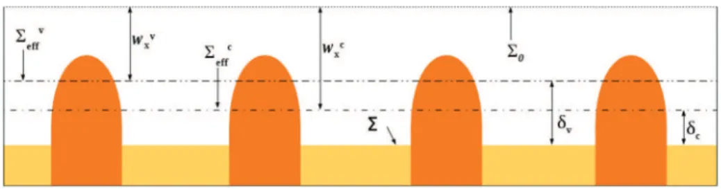
0,i (55)

Fig. 4. Schematic illustration of the position of the different effective surfaces, whereδvandδcare not normalized with respect to hr.

Following [15,30], it is interesting to look atthe modification of thisboundary conditionfor another position ofthe

effective surface.For agiveneffective surface

6

eff definedat position y

=

w,a firstorder Taylorexpansion allows usto

write u0

|

y=w

=

u0

|

y=0

+

w

∂

u0

∂

y

¯

¯

_y=0e1 (56)

whichcanberewrittenas

u0

|

y=w

=

¡

w

−

wvx

¢ ∂

u0

∂

y

¯

¯

y=0e1at

6

eff (57) bysubstitutingEq.(55).

Up tothispoint, thehomogenizationprocedureenablesto buildthe effectivemomentumboundaryconditions,which

dependonthechoiceoftheeffectivesurfaceposition.Itisseenthat atthepositiondefinedby y

=

wv

x onecanrecovera

no-slipboundarycondition(cf.Fig. 4),whichplaysanimportantroleinthemacro-scalesimulationsasshownlater.

3.2. Masseffectiveboundarycondition

Inthissection,thesamehomogenizationmethodisappliedtothemasstransferproblem.Firstorderestimateforci can

bewrittenas ci

=

c0

|

y=0

+

y

∂

c0

∂

y

¯

¯

y=0

+ ˜

ci (58)

Consequently,Eq.(26)canbetransformedinto

v

∂

c0

∂

y

¯

¯

_y=0

+

ui

· ∇ ˜

ci

= ∇ ·

¡

D

∇ ˜

ci

¢

(59)

withv

=

ui

·

e2.Themassboundaryconditionscanberewrittenas

−

n

·

¡

D∂c0 ∂y

¯

¯

y=0e2

¢

−

n

·

D

∇ ˜

ci

=

0 at

6

βσ and

6

l.i (60)

˜

ci

(

x

+

li

) = ˜

ci

(

x

)

at

6

l,i (61)

˜

ci

=

0 at

6

0,i (62) (B.C. I) c0

|

y=0

+

y∂_∂c_y0

¯

¯

_y=0

+ ˜

ci

=

ceq at

6

βγ (63) or (B.C. II)

−

nls

·

µ

D

∂

c0

∂

y

¯

¯

y=0e2

¶

−

nls

·

D

∇ ˜

ci

= −

kγceq

Ã

1

−

c0

|

y=0

+

y ∂c0 ∂y

|

y=0

+ ˜

ci ceq

!

at

6

βγ (64)

which mustbecompleted withthemomentumequations,such astheNavier–Stokesequation illustratedby Eq.(24)and

thecorrespondingboundaryconditionsillustratedbyEqs.(29)and(31).Tosolvethisproblem,asolutionforc

˜

i shouldbe

soughtbylinkingthedeviationtothemacroscopicconcentration,whichwrites

˜

ci

=

a

(

c0|y=0

−

ceq

) +

b

∂

c0

∂

y

¯

¯

y=0 (65)

wherea andb arefirst-ordermappingvariables.

SubstitutingEq.(65)intoEqs.(60),(63)and(64),weget

−

n

·

¡

D∂c0 ∂y

¯

¯

y=0

(

e2

+ ∇

b

)

¢

−

n

·

D

¡

c0

|

y=0

−

ceq

¢

∇

a

=

0 at

6

βσand

6

l.i (66) (B.C. I)

(

1

+

a

)(

c0

|

y=0

−

ceq

) + (

y

+

b

)

∂∂cy0

¯

¯

y=0

=

0 at

6

βγ (67)

or (B.C.II)

−

nls

·

³

D∂c0 ∂y

¯

¯

y=0

(

e2

+ ∇

b

)

´

−

nls

·

D

¡

c0

|

y=0

−

ceq

¢

∇

a

=

kγceq

µ

(1+a)¡c0|y=0−ceq¢+(b+y) ∂_c0 ∂y|y=0 ceq

¶

at

6

βγ (68)

andthe problemmaybe transformedintotwoindependent problemsfora andb,i.e., PbIIIa andPbIIIb aspresentedin

Appendix C.Itcanbenotedthatb

= −

y isasolutionofPbIIIbandconsequentlycicanbesimplyexpressedas

ci

=

a

¡

c0|y=0

−

ceq

¢

+

c0|y=0 (69)

Consideringu0

=

ui andc0

=

ci at

6

0,i,themassfluxbalancedescribedbyEq.(15)canberewrittenas

n0,i

· (−

D

∇

c0

) =

n0,i

· (−

D

∇

ci

)

at

6

0,i (70)

whichcanbetransformedinto

n0,i

· (−

D

∇

c0

) = −

c0

|

y=0

−

ceq A0,i D

Z

A0,i

∂

a

∂

yd A at

6

0,i (71)

whereA0,iisthesurfaceareaoftheboundary

6

0,i.Forlateruse,aneffectivereactionratecoefficientk0_effisdefinedas

k0_eff

= −

D

R

A0,i ∂a ∂yd A A0,i (72)

andtheeffectiveboundaryconditionat

6

0 canberecastinto

n0,i

· (−

D

∇

c0) = −k0_effceq

µ

1

−

c0|y=0 ceq

¶

at

60

(73)

Remarkably,theobtainedeffectiveboundaryconditionis,mathematicallyspeaking,ofareactivetype,eveninthecasewith micro-scalethermodynamicequilibrium.Ofcourse,theeffectiveboundaryconditionhasthesameformincaseIandcaseII,butthe valuesofk0

eff aregivenbyclosureproblemswithdifferentboundaryconditions,asillustratedinAppendix C.

For

6

effatanarbitraryposition y

=

w,thefirstorderestimateofthemacro-scaleconcentrationcanbedevelopedas

c0|y=w

=

c0|y=0

+

w

∂

c0

∂

y

¯

¯

¯

¯

¯

y=0 (74)

Assumingatfirstorderthat ∂c0

∂y

|

y=w

=

∂_∂cy0

|

y=0,Eq.(73)isrewrittenas D

∂

c0

∂

y

|

y=w

=

k 0 effceq

Ã

1

−

c0

|

y=w

−

w ∂c0 ∂y

|

y=w ceq

!

at y

=

w (75)

Therefore,thefollowingreactiveconditionatanarbitraryeffectivesurfaceforcaseIandcaseIIisobtained

n0,i

· (−

D

∇

c0

) = −

keffwceq

µ

1

−

c0

|

y=w ceq

¶

at

6

eff (76) with k_effw

=

k 0 eff 1

−

w_Dk0_eff (77)

Again,theremarkableresultisthat,whatevertheboundaryconditionat

6

βγ (i.e.,thermodynamicequilibriumor

reac-tive),theeffectiveboundaryconditionhasthesamereactiveform.However,itispossibletodefineaneffectivesurface

6

_effc

torecoveranequilibriumcondition,i.e.,c0

=

ceq.FromEq.(75),thepositionofthissurfaceisgivenby

wc_x

=

D k0 eff

= −

_R

A0,i A0,i ∂a ∂yd A (78)

3.3.Effectivesurfaceandeffectiveboundaryconditions

After resolution of the closure problems,it hasbeen shown that the boundary condition forthe flow problemis of

Naviertype(resultsalreadyknown)andofRobintypeforthemasstransferproblem(theoriginalpartofthispaper).Ithas

alsobeenindicated howtoestimatetheeffectiveboundaryconditionforapositionoftheeffectivesurfacedifferentfrom

6

0.Nevertheless,thethreesurfacesdefinedpreviously,

6

0,

6

_effv and

6

_effc ,arethoseofmaininterestaswillbediscussedin

Fig. 5. Unit cell geometry for the simulation (left) and illustration of roughness shape and roughness density (right).

TheobtainedgeneralformoftheeffectiveboundaryvalueproblemconsistsofPbIIandtheboundaryconditionsatthe

effectivesurface,forinstance,Eqs.(57)and(76)foranarbitrarysurfaceposition

6

eff (at y

=

w),whichbecomeEqs.(55)

and(73)whentheeffectivesurfaceisat

6

0,or

(

_u i

=

0

−

nls

·

D

∇

c0

= −

kv_effceq

³

1

−

c0 ceq

´

₍₇₉₎

whentheeffectivesurfaceisat

6

_effv ,or

½

ui

=

¡

wc_x

−

wv_x

¢

∂u0 ∂y

¯

¯

y=0e1 c0

=

ceq (80)

whentheeffectivesurfaceisat

6

_effc .

4. Effectiveparameterscalculations

The aim of thissection is to analyzethe impact of some factors, forinstance the roughnessfeatures, the Péclet, the

Schmidt andthemeanDamköhlernumbers,ontheeffectiveparameters.ThePécletandtheSchmidtnumbersaredefined

as Pel

=

urefw0x D

,

Sc

=

µ

ρ

D (81)

where,thecellheight w0x isusedasacharacteristiclength.Thereferenceflowvelocityuref ischosen asthex-component

ofthevelocityat

6

0.ThemeanDamköhlernumberwillbedefinedlater.

Dimensionless forms of closureproblem Pb III(B,s) and PbIIIa are solved to obtain the effective surface position and

boundaryconditions,withtheunitcellpresentedinFig. 5.Twoshapesofroughnessareusedinthesimulations,semi-ellipse

orroundedsquare.The heightoftheroughnesshr anditswidthbr arethetwo independentparameters.The heightand

widthoftheunitcellaredenotedasw0_x (withw0_x

=

8hr)andli,respectively.Inthefollowingsimulations, w0x andhr have

fixedvalues,whileliandbrarevariedinordertomodifyeithertheroughnessgeometryortheroughnessdensityasshown

inFig. 5.

All the following simulations are performed using COMSOL®. The linear systems are solved with the direct solver

UMFPACK, which isbasedon theUnsymmetric MultiFrontal method.The velocityfield in PbIIIa iscalculatedby solving

dimensionlesssteady-state Navier–Stokesequations.QuadraticLagrange element formulationisused fortheclosure

vari-ablesa,B andthevelocity.LinearLagrangeelementsettingsareusedforpressureanditsmappingvariables.Propermesh

qualitiesareobtainedtoensureconvergence.Forexamplefortheunitcellwith br

li

=

0

.

1,Pel

=

25 andSc

=

1,sincefurther

increase ofthenumberofdegreesoffreedomlarger than104 leadsto thevariationof

R

_A

0,i

∂a

∂yd A lessthan1%, itis

con-sideredthattheresultsare ofappropriate qualityinsuch circumstances.Giventhefactthattheunit cellgeometryunder

studyisquitesimple,itisveryeasytogetconvergedresults;thereforenomoredetailsoftheprocedureareprovidedhere.

Fig. 6. Effective surface position of6v_eff(left) and6_effc (right) for different roughness geometries and densities.

4.1. Effectofroughnessfeaturesoneffectivesurfacepositions

Inthissubsectiontheinfluencesoftheroughnessgeometryanddensityonthepositionsof

6

_effv and

6

c_effareinvestigated.

Sincewv

x andwcxarevaluesvaryingwiththechoiceof

6

0,itismoreconvenienttointroducethecorrespondingnormalized

values

δv

=

w0x−wvx

hr and

δc

=

w0

x−wcx

hr toindicate the effective positions relative tothe solid surface (see Fig. 4, where

δv

and

δc

arenotnormalizedwithrespectto hr).ResultsforfoursetsofsimulationsarepresentedinFig. 6.

In the left graph,it is observed that both the geometry and the roughness density havean impact on

δv

. One can

observethatforhigherroughnessdensities,i.e., br

li

→

1,

6

v

eff goesclosertotheroughnessheightbecausethenarrowgaps

betweenasperitiesmakeitdifficultforthefluidtoflowthrough.Theupperlimitof

δv

isoneandisnearlyreachedforthe

thinsemi-ellipseandtheroundedsquaresbecausetheirroughnessshapesaresteep.Forroughnessescloseenoughtoeach

other,theheterogeneous surface hasa similarbehavior interms ofmomentum transportasa smooth surface locatedat

theheightoftheroughnesses.Forsmootherroughnesses,thelimitcasewheretworoughnessesareadjacentgivesavalue

of

δv

smaller than one asthe fluid can still flow partially between the roughnesses.The three sets of simulations with

semi-ellipseshapealsoshowthatthinroughnessescreatemoreresistancetotheflowthanwiderones.Thecurvesexhibit

anotherlimit when br

li

→

0.Evenifthe twoneighboring asperitiesare farenough fromeach other,e.g.,li

=

50hr in this

case,theroughnessesstillhavesomesmallimpactontheflowand

δv

tendstowards0

.

1hr.

In the right graph of Fig. 6, the negative values of

δc

mean that

6

_effc locates inside the solid part. The presence of

insolublematerialsmakestheaveragedconcentrationon

6

smallerthantheequilibriumconcentration,therefore

6

_effc must

belocatedbeneath

6

torecoverthethermodynamicequilibrium.Similartothecasewithno-slipcondition,bothroughness

shape androughnessdensityare playinga roleon

δc

. However, onecan observe thatthe three setsof simulations with

semi-ellipseshapesare superposed,indicatingthat thewidthoftheroughnesshaslittleimpacton

δc

foragivenratioof

br

li.Oneseesfromtheseresultsthat

δc

tendstowards

−∞

whentheratio

br

li increasestowardsone,independentlyofthe

roughnessgeometry.For br

li

→

1,thesolidsurfaceincontactwiththefluidismainlyformedbytheinsoluble materialand

littlemasstransferoccursbetweenthesolidandthefluid,whichmakes itdifficulttorecoverthermodynamicequilibrium

effectiveboundarycondition.Theupperlimit of

δc

isequaltozeroandisobtainedforlowroughnessdensity(br

li

→

0).In

thiscasethesolid–liquidinterfacebehaveslikeahomogeneoussolublesurface.

4.2.Thermodynamicequilibriumcase(B.C.I)

Inthissubsection,the dependenceofkv_eff on differentfactors isinvestigatedfirst. Simulations areconductedfor both

advective–diffusivemasstransportregimeandpurelydiffusive regime.Inthelattercase, theeffectivereactionrate

coeffi-cientis denotedaskv

effdiffu.Theflat partofthe solid–liquidinterface isunderthermodynamic equilibrium. Theroughness

shape issemi-ellipse witha height of hr.The other geometric parameters ofthe unit cell are w0x

=

8hr, br

=

0

.

5hr and

li

=

5hr. Theratioof k v eff kv effdiffu

asafunctionofPel andSc isplottedinFig. 7.

Oneseesinthefigure that k

v

eff kv

effdiffu

increasesgloballywithPel andSc,whichmeansthattheflowhasastrongerimpact

Fig. 7. Ratiobetweenkeffv withadvectionanditsvalueinthepurelydiffusivecase,asafunctionofPelandSc.Semi-ellipseroughnesswasusedwith

br=0.5hrand blir=0.1.

effectivereactionratecoefficientwithadvectionisnearlythesameastheoneunderapurelydiffusiveregime.ForSc

<

0

.

1,

the difference betweenkv

eff andkveffdiffu isless than 1% forPel

<

1000.Consequently, themass transport problemcan be

simplifiedintoapurediffusioncaseinsuchcircumstances,producinganerrorsmallerthan1%.ForthecaseswithSc close

to 1, k

v

eff kv

effdiffu

reachesamaximum athighPel values,thendecreases andincreasesagain. Forhigher Sc theratioincreases

withPel withdifferentrateexceptforSc

=

100 andSc

=

1000 thatare superposedonthestudied rangeofPel.One has

topayattentionthattheconsideredsituationinthisstudyislaminarflowwithinaboundarylayer.Thereforeforthecases

withsmallSc,theconsideredPel shouldnotbetoolarge.

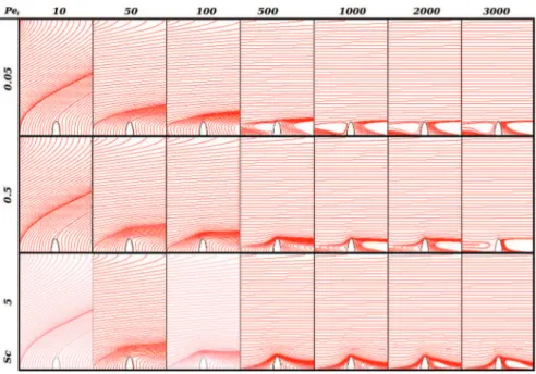
Toillustratethedifferentregimesbetweenmasstransportgovernedbydiffusionorbyadvection,thestreamlinesofthe

totalflux ofa versusSc andPel areplottedinFig. 8.WithsmallPel (10and50),thevariationofSc onlyhassome small

impact onthestreamlines,whichillustratestheweak influenceoftheflowonthemassexchange atthe reactivesurface.

Thevalueofkv_effisthereforeclosetothevalueinthepurelydiffusivecase(withadifferenceless than1%)asillustratedin

Fig. 7.WithlargerPel values,increasingSc (i.e.,increasingtheviscosity)delaystheoccurrenceofrecirculationsclosetothe

roughsurface,whichexplainsthemaximumvaluesobservedinFig. 7.Therecirculationsfirstlimitmasstransporttowards

thesolublematerial,andthenenhanceitforincreasing Pel,correspondingtothedecreaseandincrease of

kv eff kv effdiffu afterthe maximumvalues.

In asecond set ofsimulations,the influenceof therough surface geometryon k

v

eff kv

effdiffu

isinvestigatedby changing the

roughnessdensity.FromtheresultspresentedinFig. 9,ahighroughnessdensityleadstoadelayinthetransitionbetween

theadvectiveanddiffusiveregime.Onecanobserveforexamplethatfor br

li

=

0

.

4 and

br

li

=

0

.

5,theflowalonehasasmall impactontheeffectivereactionratecoefficient(lessthan1%)evenforhighPel values.Intheseconfigurations,kveffdiffu isa

goodestimateofkv

eff.Astheroughnessdensitydecreases,

kv

eff kv

effdiffu

increasesbecausetheflowcanpassthroughtheroughness

moreeasily,andthereforemoresolidsurfaceunderthermodynamicequilibriumisavailableformasstransfer.

4.3. Thecaseofareactivesurface(B.C.II)

Inthissubsection,theflatpartofthesolid–liquidinterfaceisreactive.Tostudytheimpactofthechemicalfeatureson

the effectivereaction ratecoefficient, some parameters are first introduced. Letkσ denote the reactivityat surface

6

βσ .

One should note that kσ isequal to zeroin this study since the

σ

-phase is non-reactive. The surface average reaction

ratecoefficientforaheterogeneoussurfacecanbeapproximatedask

ˆ

=

kγAβγ+kσAβσ

Aβγ+Aβσ ,with Aβγ and Aβσ representingthe

surfaceareasof

6

βγ and

6

βσ ,respectively.Accordingtothemassconservationfrom

6

to

6

effv ,thesurfaceaveragereaction

ratecoefficientat

6

_effv can beestimatedask

ˆ

v

=

kγAβγ+kσAβσ

Av ,with Av denotingthesurface areaof

6

v

eff.The structureof

the concentration field inside the domain will depend on the ratio between reaction characteristic rates and diffusion,

correspondingtoameanDamköhlernumberdefinedas

c

Da

=

kwˆ 0x

Fig. 8. Total flux streamlines of closure variable a for different Sc and Pel. The roughness shape is a semi-ellipse with br=0.5hrand blri =0.1.

Fig. 9. Ratiobetweenkv

eff withconvectionanditsvalueinthepurelydiffusivecase,asafunctionofthelocalPécletnumber,for differentroughness densitiesgivenbybr

li andSc=0.1.

Theroughnessshape underconsiderationissemi-ellipse.Theheightandwidthoftheroughness,aswellastheheight

of the unit cell remain unchanged, withbr

=

0

.

5hr and w0x

=

8hr. Tworoughness densities, li

=

5hr andli

=

10hr, are

considered.

Theresultsof k

v

eff

ˆ

kv versus

c

Da arepresentedinFig. 10fordifferentPel andSc.Forsmall

c

Da,

kv

eff

ˆ

kv tendstowardsonedespite

of the flow properties. In such circumstances, the characteristic time ofreaction is long compared to the mass-transfer

kinetics,andthe processis consequentlylimitedby reaction.Withtheincrease of

c

Da,masstransferbecomesinsufficient

andtheprocessisthereforelimitedbythemasstransport.Inotherwords,k

ˆ

v_{tendstoinfinitywhilek}v

effremainsaconstant,

leadingto k

v

eff

ˆ

kv tendingtowardszero.

Forafixedroughnessdensity,li

=

5hr orli

=

10hr,whenPel

=

1,anincreaseofSc doesnotaffect kv

eff

ˆ

kv sincethecurves

ofSc

=

1 andSc

=

1000 aresuperposed,whilewhenSc remainsunchanged,theincreaseofPel delaysthedecreaseof

kv

eff

ˆ

Fig. 10. Theratioofeffectivereactionratecoefficientkv

effoverthesurfaceaveragereactionratecoefficientkˆv,asafunctionofthemeanDamköhlernumber, withdifferentsurfacegeometries.

Fig. 11. The functionality of the effective Damköhler number Dav

effwith the mean Damköhler numbercDa.

TheseresultsillustratethatonlyrelativelylargePel havesomeimpactonkv_eff,consistentwiththefollowingdiscussionabout

Da_effv andwiththeresultsillustratedlaterbyFig. 12.Forthegeometrywithli

=

10hr,thedecreaseof kv

eff

ˆ

kv isdelayedsince

thefluid canflowthroughtheroughnessmoreeasily thusenhancemasstransfer.Therefore,itcanbe concludedthatthe

roughnessdensity,theflowpropertiesintermsofPel andthechemicalfeaturesintermsof

c

Da haveanimportantinfluence

onkv eff.

Sinceitisnotconvenienttousetheratio k

v

eff

ˆ

kv when

c

Da islargebecauseittendstozero,aneffectiveDamköhlernumber

defined as Dav_eff

=

k

v

effw0x

D is introduced to indicate the evolution of k

v

eff with

c

Da. Results are plottedin Fig. 11. Da

v eff is

proportional to

c

Da before itreachesa plateauwhenmass transportbecomesthe limitingfactorofthechemical process,

consistent withtheresultsofasimilar analysisin[14].Quantitatively,whenPel remainsunchanged, Daveff forli

=

10hr is

twice aslargeasforli

=

5hr inthelimitoflargeDa.

c

Thisisalsoexplainedby thefactthatmasstransportislimitingthe

process under large

c

Da andincreasing theproportionof the dissolving phaseis equivalentto increasing masstransport.

Moreover, flow and roughnessdensity haveonly a smallimpact on Da_effv forsmall

c

Da becausein such circumstances it

Fig. 12. Ratiobetweenkv

effwithadvectionanditsvalueinthepurelydiffusivecase,asafunctionofthelocalPécletnumberandfordifferentSchmidt numbers.Theroughnessshapeisasemi-ellipsewithbr=0.5hrandblri =0.1.

roughnessdensityundersmall

c

Da and decreaseswithroughnessdensityunderlarge

c

Da,whichisduetothetransitionof

thelimitingfactor.

Finally,theimportanceofmasstransportbyadvectionisstudiedbyplotting k

v

eff kv

effdiffu

versusPel fortwo

c

Da valuesandfor

differentSc,asshowninFig. 12.Oneseesfromthefigurethatwiththeincrease ofPel,theratio

kv_eff kv

effdiffu

tends toincrease

since the advectionterm becomesmore important.The curves withthe same Sc havesimilar trends butwithdifferent

magnitudes.In the case withhigher

c

Da, the role of advection ismore important andthe transitions from the diffusive

regime totheadvectiveregime take placeatsmallerPel.ForthecurveswithSc

=

0

.

1,the increaseshappen atrelatively

largePel andcanleadtolarger

kv

eff kv

effdiffu

thanthecurveswithSc

=

10 insomecircumstances,becausethegrowthof k

v

eff kv

effdiffu

withSc

=

10 slowsdownatabout3000

<

Pel

<

7000.Thistrendissimilartotheresultsobtainedwiththethermodynamic

equilibriumboundary condition. Recirculations closeto the rough surface have a similar impact, first limiting the mass

transporttowardsthereactivesurfaceandthenenhancingit.Tosummarize,toestimatekv

effbykveffdiffuwillproduceanerror

lessthan5%forthestudiedcaseswithDa

c

=

1,becausethereactionratecoefficientisthelimitingfactorofprocessandthe

flowpropertieshavenegligibleimpact.Onehastobecarefultorepresentk_effv byk_effv

diffu atlarge

c

Da sincetheflowproperties

canhavesignificantinfluenceinsuchconditions.

5. Applicationoftheeffectivesurfacemodel

AsintroducedinSection3,therearedifferentpotentialchoicesforthepositionoftheeffectivesurface,e.g.,thefictive

surface

6

0, surface

6

_effv which recovers theno-slip boundarycondition, surface

6

_effc whichrecovers the thermodynamic

equilibriumcondition, oranyarbitrarylocation. Inthissection the objectiveis toidentify themostappropriate effective

surfacebyinvestigatingtheerrorsbetweendirectnumericalsimulations(DNSs)overtheoriginalroughsurfaceand

simula-tionswiththeeffectivesurfacemodel.Twosituationsareconsidered,typicalofthedevelopmentofamassboundarylayer

overaroughsurface.

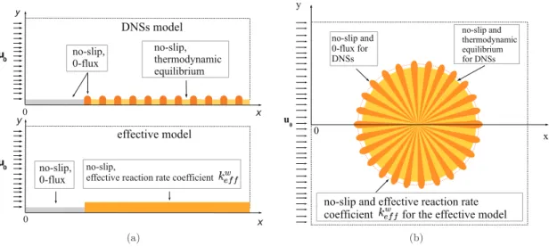
The first application corresponds to a boundary layer over a rough wall parallel to the flow. The original model for

DNSsisillustratedby theupperdrawingofFig. 13(a).Thecharacteristiclengthofthesystemusedtonormalizethespace

variablesisHÄ,i.e.,L,theheightoftheglobaldomain.ThesystemisW

=

3HÄwide.Ashortflatzoneissetwithalength

of0

.

5HÄ beforethe roughsurface inorderto havean alreadydevelopedboundarylayer, whichiscloserto theperiodic

boundaryconditionhypothesis statedpreviously.Inaddition,the roughnessheightis chosen tobe smallenough tohave

ǫ

=

_Ll

=

0

.

1 andl

=

8hr.Theroughnesshasashape ofsemi-ellipsewithbr

=

0

.

5hr.Intermsofgeometryfortheeffective

models,theflatsurfaceattheentranceremainsunchangedandtheoriginalroughsurfaceisreplacedbyasmootheffective

one.ThelowerdrawinginFig. 13(a)givesanexampleoftheeffectivemodelwithno-slipconditionattheeffectivesurface.

Theoriginal flatsurface andtheeffectivesurface are connectedbya smallstep.Itis clearthatsome assumptions ofthe

homogenizationarenotvalidinthisparticulararea,whichisasingularity(no-periodicity,etc.).Specificdevelopmentscould

Fig. 13. Schematicrepresentationofthecomputationaldomain:DNSsovertheheterogeneoussurfaceandthefirstordereffectivemodels(application1in (a)andapplication2in(b)).

In the second application, the boundary layer develops on a rough cylinder perpendicular to the flow. As illustrated

in Fig. 13(b),the rough surface in theDNSs is replacedby the smooth circular surface inthe effectivemodel.Since the

considered geometry issymmetric withrespectto x-axis, onlythe transport inthe upperhalf domainis simulated.The

characteristiclengthofthesystemusedtonormalizethespacevariablesisL,thecylinderdiameter.Theheightofthehalf

domainisHÄ

=

1

.

5L andthewidthisW

=

2

.

5L.

DNSsareperformedusingdimensionlessformsofPbIequationswithB.C.I.Fortheeffectivemodel,theclosureproblems

PbIII(B,s) andPbIIIa illustratedintheappendicesaresolvedfirsttoobtaintheeffectivesurfacepositionandtheeffective

boundaryconditions,assummarizedinsubsection3.3.Thentheeffectivemacro-scale problemPbII issolved usingthese

obtainedeffectiveboundary conditions.Similarnumericalsettings wereused asinthelast section.Convergence analyses

wereconductedforeachcomputationtoguarantytheresultsquality(seeSupportInformation).

5.1. Application1:boundarylayeroveraroughwallparalleltotheflow

Thewaytoquantifythedifferencesbetweenthetwosimulationsistocalculatetheerrorontheintegrationofthetotal

mass fluxover thesolid–liquid surface,called QDNS fortherough surface and Qeff fortheeffectiveone. Simulationsare

done forflows with ReL

=

1 and ReL

=

50,with two roughnessdensities: b_lr_i

=

0

.

5 and b_lir

=

0

.

1. The relative errors on

the totalmassflux are plottedin Fig. 14fordifferenteffectivesurface positions.Foreffective surfaceata positionlower

than2

.

5hr,therelativeerrorcommittedby themodelissmallerthan1%.Athighereffectivesurfacepositionsandforthe

differentReynoldsnumbers,theerrorincreaseswhenincreasingthepositionoftheeffectivesurface.Onecanalsoobserve

thattheroughnessdensityhaslittleimpactontheerrorcomparedtotheinfluenceofReL.Increasingthedistancebetween

roughnesses byafactoroffiveonlyincreasestheerrorbylessthan 1%,whileincreasingReL from1to50nearlydoubles

theerror.Forthedifferentflowconditionsorgeometry,aminimumvalueoftherelativeerrorisobtainedaround yeff

=

hr.

Itisclosestto

6

_effv amongtheparticulareffectivesurfacepositionsdiscussedbefore.

To demonstratethe representativeness ofthe effectivemodelwith theeffective surface locatedat

6

_effv , theresults of

DNSs and the firstorder effective model are compared interms of velocity,concentration fieldsand the distribution of

massfluxoverthereactivesurfaceasillustratedinFigs. 15 and16,respectively.Resultswiththeeffectivesurfaceat

6

0are

alsoshowninthesefigurestoillustratethediscrepanciescreatedbythelargestepbetweentheflatzoneandtheeffective

surface.

IntheuppergraphofFig. 15,onecanobservethatthevelocitycontoursobtainedbyDNSs(solidline)andthoseobtained

withthefirstordereffectivemodelwithan effectivesurfaceat w0x−wvx

L i.e., at

6

v

eff,are overlapped,withnegligibleerrors.

Thisisconsistentwithpreviousfindings intheliterature forthemomentumtransport problem.Resultswiththeeffective

surface at wvx

L (dotline),i.e., at

6

0,give thegood trendbutare not preciselyrepresentingtheDNSs velocityfield. Asfor

concentrationcontours,oneseesinthelowergraphofFig. 15thatthoseobtainedwiththeeffectivesurfaceat w0x−wxv

L are

also well superposed withthe DNSs results,except inside the smallentrance region where the conditions forupscaling

breakdownasdiscussedpreviously.Quantitatively,thiscreatesa smallandratheracceptablediscrepancyof0.07%onthe

total mass flux. The iso-concentration contours obtained withthe effective surface at w0x

L show some discrepancies that

increasewith x_L,leadingtoarelativeerroronthetotalmassfluxofaround6.2%.

InFig. 16,thedistributionofthenormalmassflux,q,alongthereactive surfacesinthe effectivemodelwith

6

_effv and

Fig. 14. RelativeerroronQeffcomparedtoQDNS,fordifferentpositionsoftheeffectivesurface,withdifferentsurfacegeometries,Sc=1 andtwovalues ofReL.

Fig. 15. Dimensionlessvelocityfield(uppergraph)andconcentration(lowergraph)contoursfortheinitialroughdomainandtwoeffectivesmoothdomains, withanentrancedimensionlessflowvelocityof1,ReL=25 andSc=1.

Fig. 16. Normalfluxalongthe reactivesurfacesfortheinitialroughdomainandtwoeffectivesmoothdomains,withanentrancedimensionlessflow velocityof1,ReL=25 andSc=1.

tobeaveragedforeachli.TheresultsoftheDNSsandtheeffectivemodelwith

6

_effv showagoodagreement.Forthemodel

withtheeffectivesurface at

6

0,q distributiondiffersfromtheDNSsintheentranceregion afterthe step.Thisismainly

theconsequenceofthediscrepanciesobservedinthevelocityfield.

5.2. Application2:roughcylinderinalaminarflow

This second caseillustrates the accuracy of the effective model fora more complex configuration than the previous

application. Simulations are done for a flow with ReL

=

0

.

1 and Sc

=

1000,with 50 roughnesses distributed uniformly

overthecylindersurface and

ǫ

=

0

.

1.InthetwographsofFig. 17,one canobservethatbothvelocity contours(top)and

concentrationcontours(bottom)obtainedbyDNSs(blacksolidline)andwithaneffectivesurfaceat

6

_effv (bluedashedline)

areoverlapped,withnegligibleerrors.TheerroronQ islessthan0.1%,provingagainthevalidityofthefirstordereffective

surfacemodel.Thiserrorremainssmallerthan0.1%evenbyincreasing

ǫ

to0.5(thescaleseparationassumptionisnomore

valid).However forReL

=

1, Sc

=

1000 and

ǫ

=

0

.

5,themodelstarts to showsome limitationsandgivesresultswithan

erroraround3%.

5.3. Effectiveparametersestimates

Intheselast paragraphs,potential estimatesofthe effectivepropertiesare discussedinordertoreduce computational

costs,takingapplication1asanexample.AsmentionedpreviouslyinSection4,forahighroughnessdensitytheeffective

surfacepositionisclosetotheroughnessheight.Onefirstpossibleapproximationistosettheeffectivesurfacepositionat

theroughnessheight,usingano-slipboundaryconditionandthenusetheeffectivereactionrateobtainedforaneffective

surface at hr, which will be called

6

_effr . Relative errors committedon the total mass flux using this approximation are

comparedtotheonewiththecorrecteffectivemodelwith

6

_effv .ResultsareassembledinTable 1forReL

=

25 and Sc

=

1,

andforroundedsquare roughnesseswithbr

=

hr.Theapproximatedmodelgivesresultswithrelativeerrorsless than1%

even for roughnessdensities aslow as 0.2, i.e., br

li

=

0

.

2 with

δv

=

0

.

73. This firstapproximation givesgood results for

certainroughsurfacegeometriesandwillsavecomputationaltimeastheclosureproblemfortheflowdoesnotneedtobe

solvedanymore.

Inadditiontothisfirstestimate,anapproximationcanbemadeontheeffectivereactionrateaswell.IntherangeofReL

usedfortheglobalsimulations(1to1000),thecorrespondingmicro-scalePécletnumberwillnotexceed100forSchmidt

numbersbelow10.FromtheparametricstudyofSection4,ithasbeenobservedthattheeffectivereactionrateobtained

forpurediffusioncanbeagoodapproximationoftheeffectivereactionratewithflow.Asaresult,PbIIIawithB.C.Icanbe

simplifiedintoapurelydiffusiveoneintheseapplicationranges.Forexample,thelargestdifferencebetweenerrorsonQ ,

committedwithandwithoutaccountingfortheflowinkv

eff is0.002(obtainedwith

br li

=

0

.

1,ReL

=

500 andSc

=

5 which hasaratio k v eff kv effdiffu

≈

1

.

02).

Tosumup,allthesenumericalresultsdemonstratetheefficiencyofusinganeffectivesurfacemodel,characterizedbya

homogeneousandsmoothsurface,toreproducetheflowandreactivemasstransportoveraheterogeneousroughsurfaces,

withagoodaccuracy.TheuseofestimateswithoutsolvingPbIII(B,s)canhelptogaincomputationaltime,butmayneedto

Fig. 17. Dimensionlessvelocityfield(top)andconcentration(bottom)contoursfortheinitialroughdomain andtheeffectivesmoothdomain,withan entrancedimensionlessflowvelocityof1,ReL=0.1 andSc=1000.

6. Conclusion

The concept of effective surface has already proven its usefulness for several transport mechanisms. The main

con-tribution ofthis paper concerns mass (andmomentum) transfer fora laminar flow over a heterogeneous rough surface

characterizedbymixed boundaryconditions.Averyimportantconstraintnecessarytodeveloptheeffectivesurfaceconcept

isthe separationofscales betweenthe globalboundary layerthicknessandthe zone ofinfluenceof thesurface

hetero-geneitieswithin thatboundarylayer.Additional assumptionsweremade, likemicro-scalepatternperiodicity,whichcould