OATAO is an open access repository that collects the work of Toulouse
researchers and makes it freely available over the web where possible
Any correspondence concerning this service should be sent
to the repository administrator:
tech-oatao@listes-diff.inp-toulouse.fr
This is an author’s version published in:
https://oatao.univ-toulouse.fr/26703
To cite this version:
Fabre, Clément and Simeoni-Sauvage, Sabine and Probst, Jean-Luc
and Sanchez-Pérez, José Miguel Global-scale daily riverine DOC
fluxes from lands to the oceans with a generic model. (2020) Global
and Planetary Change, 194. 103294. ISSN 0921-8181
Open Archive Toulouse Archive Ouverte
Official URL :
Global-scale daily riverine DOC fluxes from lands to the oceans with a
generic model
C. Fabre
⁎, S. Sauvage, J.-L. Probst, J.M. Sánchez-Pérez
⁎Laboratoire écologie fonctionnelle et environnement, Université de Toulouse, CNRS, INPT, UPS, Toulouse, France
Keywords: DOC Global scale Generic model Daily Riverine exports A B S T R A C T
The export of riverine dissolved organic carbon (DOC) to the oceans is determinant in carbon exchanges of the
estuaries and oceanic food webs. Past research returned a global DOC export around 160–450 TgC.yr−1 by using
complex process-based models or yearly average estimates that could have been misjudged. In this study, we try to understand the complex processes explaining daily DOC exports among 341 exoreic watersheds covering 71% of freshwater flows to the oceans. Based on a dataset of DOC concentrations among rivers at the global scale, we were able to link DOC concentrations to daily discharge, the ration between the soil organic carbon content and the amount of precipitations and the average air temperature in the watersheds. We have found a global riverine
DOC flux of 131.6 TgC.yr−1 based on daily data and a generic model. Tropical and cold watersheds are the main
contributors with 49.5% and 33.3% of the global riverine DOC flux on the two last decades while temperate, semi-arid and polar basins represent 15.9%, 0.7% and 0.6%, respectively. Temporal exports range from 0.1 to
0.16 TgC.day−1 in tropical areas, 0.03–0.32 TgC.day−1 in cold areas and 0.03–0.08 TgC.day−1 in temperate
areas. Atlantic and Arctic oceans receive the most important fluxes (0.12–0.2 and 0.01–0.26 TgC.day−1). In a
climate change context, this generic equation could be introduced in hydrological modelling tools to predict future DOC fluxes trends.
1. Introduction
Rivers represent the primary connection between land and sea in the different biogeochemical cycles (Ciais et al., 2013). In the global carbon cycle, riverine exports into oceans are sources of many biolo-gical processes (Drake et al., 2017). Hence, organic carbon is a main driver of greenhouse gas emissions in hydrosystems by respiration or denitrification (Ciais et al., 2013). Riverine organic carbon is involved in other biogeochemical cycles and can transport pollutants (Drake
et al., 2017; Vitale and Di Guardo, 2019). In the 80s and 90s, the
un-derstanding of the global exports of organic carbon from rivers to the oceans was a central concern (Ludwig et al., 1996; Meybeck and
Vörösmarty, 1999 and references therein). These exports were more
and more studied in the past years as their understanding, quantifica-tion and predicquantifica-tion are essential in this time of global changes (Ciais
et al., 2013). Research on these exports helps to understand better the
impacts on the estuaries and oceanic food webs (Ward et al., 2017). Past studies already focused on organic carbon exports from the major river basins in the world with an estimate between 0.3 and 0.6 PgC.yr−1 (1 Pg = 1015 g) based on a set of 60 to 80 big rivers (Ludwig
et al., 1996; Cole et al., 2007; Drake et al., 2017).
Dissolved organic carbon (DOC) is one of the two forms of organic carbon with the particulate organic carbon (POC; Hope et al., 1994) and plays an intricate role in the ecosystems (Ward et al., 2017). DOC originates mainly from soil leaching (Meybeck, 1993). From 3 to 35% of the riverine DOC is labile (Ittekkot and Laane, 1991; Søndergaard
and Middelboe, 1995). Various biogeochemical processes alter the DOC
pool in riverine, estuarine and coastal environments, e.g., assimilation or sedimentation (Drake et al., 2017). While the labile part of POC is higher (10 to 50%), the DOC fate needs more interest than POC as it is generally more concentrated in rivers and estuaries (Spitzy and
Ittekkot, 1991). Plus, microbial communities are preferentially
con-suming DOC (Raymond and Bauer, 2001) and the global oceanic DOC pool represents one of the largest reactive reservoirs of carbon at the global scale (Schlesinger, 1991).
As various short-time processes affect DOC through the hydrological cycle, existing estimates of riverine DOC fluxes based on interannual exports may not reflect reality, especially in watersheds presenting flash floods. These interannual DOC fluxes do not include temporal varia-tions of DOC concentravaria-tions and could misestimate real fluxes exported to the oceans. Considering daily DOC concentrations into models should improve estimations of global DOC fluxes from exoreic
⁎Corresponding authors.
= +
DOC Q
Q
[ ] .
with Q, the specific discharge in millimetres. The two parameters α and β represent a potential of maximum DOC concentration we could find at the outlet of the watershed and the discharge at which the DOC concentration is half of the maximum DOC concentration that aims an asymptote, respectively. The equation calculates a daily average DOC concentration based on daily discharge. It has already returned good
results in an Arctic basin (Fabre et al., 2019). In this study, we intend to test the validity of this model to large watersheds presenting various soils and climatic characteristics.
2.3. Acquisition of the equation parameters
For each of the 74 exoreic rivers, we statistically determined the best parameters of the equation with non-linear regressions. We used nonlinear least squares estimations to fit the model. These functions determine the weighted least-squares estimates of the parameters of a nonlinear model and return the best set of parameters. In other terms, the functions try to find the best settings that minimize the following sum: = = S ([DOC] [DOC] ) i n obs i sim i 1 , , 2
with [DOC]obs, i the observed DOC concentration and [DOC]sim, i the
simulated DOC concentration at day i.
To test the fitting, we decided to keep the stations where more than eight observations of DOC concentrations were available to keep the stations that accurately represent all the hydrological conditions. We judged the fitting acceptable when the coefficient of determination (R2) between observed and simulated DOC fluxes was higher than 0.35.
2.4. Validity of the temporal representations
To validate the model, we used various indices comparing our predicted values of DOC concentrations and fluxes with observed data. Three indices were selected to test our equation: the Nash-Sutcliffe ef-ficiency (NSE) index, the coefficient of determination (R2) and the percent of bias (PBIAS). These indices are detailed in Moriasi et al.
(2007, 2015). NSE ranges from -∞ to 1. NSE values higher than 0.5 are
judged satisfactory for hydrological daily time step modelling. R2 ranges from 0 to 1, with higher values indicating less error variance. R2 greater than 0.5 are typically considered good and values greater than 0.3 are regarded as acceptable for daily biogeochemical modelling
(Moriasi et al., 2015). PBIAS expresses the percentage of deviation
between simulations and observations, so the optimal value is 0. PBIAS can be positive or negative, which reveals model underestimations or overestimations, respectively (Moriasi et al., 2007).
2.5. Representation of the DOC temporal variations
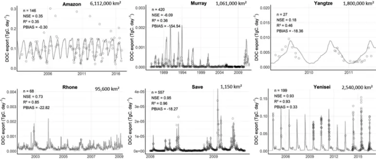
We decided to show the temporal validity of the equation on six watersheds presenting various sizes and different climate and soils conditions: The Amazon River (6,112,000 km2) for the tropical zones, the Murray River (1,061,000 km2) for the semi-arid climate, the Rhône River (95,600 km2), the Yangtze River (1,800,000 km2) and the Save River (1150 km2) for the temperate zones and the Yenisei River (2,540,000 km2) for the cold climate. We selected three rivers for one climate zone to test the validity of the equation in front of the change of scale. We also checked the spatial validity of the equation inside a watershed by validating the equation in tributaries where data were available, e.g., the Save River in the Garonne basin.
2.6. Relations between the DOC equation parameters and environmental variables
The parameter α could correspond to a potential of DOC that can be found in the river and then could be linked to the organic carbon content in soils. The parameter β represents the speed to reach the maximal DOC concentration in the watershed. The water regime or physical variables influencing this speed could explain this parameter. We produced Principal Component Analyses (PCAs) with environ-mental variables to verify these hypothetic relations. In this way, we watersheds. DOC exports were modelled at the continent or the ocean
scale (Martins and Probst, 1991; Kicklighter et al., 2013) as well as globally (Ludwig et al., 1996; Probst et al., 1997; Dai et al., 2012;
Nakayama, 2017) but these works were generally done with annual
time step empirical equations or with complex process-based models. Past research tried to link the DOC concentrations with appropriate environmental variables such as wetland or peat coverage (Hope et al.,
1994; Gergel et al., 1999; Ågren et al., 2008), C:N ratio (Aitkenhead and
McDowell, 2000) or soil organic carbon content (Aitkenhead et al.,
1999). Tao (1998) and Raymond and Saiers (2010) found a correlation
between DOC concentrations and discharge. At a global scale, the DOC modelling efforts have returned interannual physiography-driven models based on the runoff, the organic carbon content in the soil profile and the average slope of the basin (Ludwig et al., 1996; Huang
et al., 2012; Li et al., 2017) or based on climate classifications (Huang
et al., 2012). Recently, process-based models were applied to estimate
the global carbon budget, including the organic carbon exports to the oceans (Nakayama, 2017). Thus, different methods estimated the global riverine DOC exports around 0.2 PgC.yr−1 (Ludwig et al., 1996; Dai
et al., 2012; Ciais et al., 2013; Li et al., 2017). Still, the knowledge gap
is deep in modelling global riverine DOC exports from exoreic basins. This paper proposes a new method to quantify DOC fluxes at the wa-tershed and the global scale by calculating daily DOC concentrations with a generic model. The objectives of this study are i) to propose a modelling approach to quantify daily DOC concentrations and fluxes at the watershed scale with simple parameters related to environmental variables and ii) to estimate the global DOC exports to the oceans at a daily time step.
2. Methods
2.1. Watersheds database
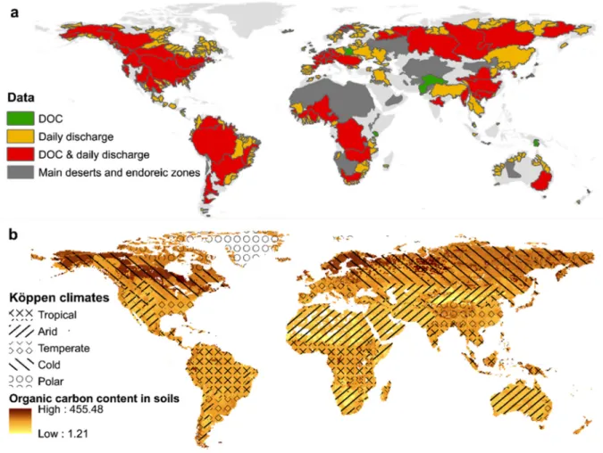
To validate the equation, we propose to study it in various water-sheds based on the data availability and the soil and climatic disparity. Most of the selected rivers are in the biggest in terms of draining area and discharge around the world. We collected data from various ex-isting databases and past projects mainly in the 1990–2015 period to constitute a panel of rivers on the whole world. Fig. 1 shows the wa-tersheds distribution, and Table 1 details the data sources. In this way, this study integrates 74 exoreic watersheds with daily DOC data. They represent 35% of the world land surfaces (Fig. 1a).
To predict the riverine DOC fluxes exported to the oceans at a global scale, we assembled daily discharge data from various databases for most of the rivers presented in Fig. 1a. Table 2 details the different databases and projects used in this paper.
2.2. Details on the DOC equation
A relation between DOC concentrations and daily discharge was highlighted by analyzing the previous dataset. The DOC concentrations reach an asymptotic value even if the discharge continues to increase. This “saturating curve” has already been brought to light in past re-search (Tao, 1998; Raymond and Saiers, 2010). In this study, we decided to adapt the Michaelis–Menten equation (Johnson and Goody, 2011) to predict the riverine DOC concentration ([DOC]) in milligrams per litre (mg.L−1) by correlating it with discharge (Q) as followed:
extracted different environmental variables from global datasets for the watersheds presenting DOC data. These variables were identified to be possibly correlated to the DOC exports and are detailed below: − Dominant Köppen-Geiger climates in the watersheds were
de-termined based on a 1950–2000 average global distribution of the
climate zones from Rubel and Kottek (2010) presented in Fig. 1b. − Average organic carbon content in the first meter of the soils (ORGC; g.m−3) and average sand content in soils (Sand) came from the Harmonized World Soil Database (Batjes, 2009) with a resolution of 30 arc sec. Fig. 1b shows the soil organic carbon content distribution at a global scale.
Fig. 1. a) Representation of the main watersheds on Earth and their available data on DOC concentrations and daily discharge. The delineation of the basins comes
from the FAO (2006). b) Representation of the organic carbon content in soils in g.m−3 based on the Harmonized World Soil Database (Batjes, 2009) and the Köppen
climate distribution (Rubbel and Kottek, 2010).
Table 1
Sources of the DOC data. n represents the number of rivers by Köppen climate group without including the tributaries. The streams in italic are tributaries of another main river of the dataset. The watersheds in bold are the ones presented in the paper to test the reliability of the equation in each Köppen climate group.
Climate group n Basins Sources
Tropical 9 Amazonand its tributaries, Congo and its tributaries, Fly, Godavari, Maroni,
Orinoco, Oyapock, Sao Francisco, Volta Araujo et al. (2014), Balakrishna et al. (2006), Moreira-Turcq et al. (2003), Observation Service SO HYBAM (2020), Paolini (1995), Spencer et al.
(2016), United Nations Environment Programme (2018)
Semi-arid 11 Chubut, Colorado (Pacific), Gambia, Hwang Ho, Indus, Missouri, Murray,
Niger, Orange, Rio Colorado, Rio Grande, Tana Araujo et al. (2014), Brunet et al. (2005), Geeraert et al. (2017), Hartmann et al. (2014), Ittekkot and Arain. (1986), Lesack et al. (1984), Martins and
Probst (1991), Ran et al. (2013), Stackpoole et al. (2017), Tao (1998), United Nations Environment Programme (2018), Wang et al. (2012)
Temperate 31 Aare, Alabama, Arkansas, Brazos, Danube, Ebro, Elbe, Gallegos-Chico,
Garonne, Irrawaddy, Ishiraky, Kiso, Klamath, Loire, Lys, Meuse, Mississippi,
Moselle, Ohio, Parana, Po, Rhine, Rhone, Rio Negro, Sacramento, Saone,
Savannah, Save, Schelde, Seine, Si Kiang, Song Hong, Stikine, Thames, Vistula, Weser, Yangtze, Zambezi
Bao et al. (2015), Bird et al. (2008), Bowes et al. (2017), Centre for Ecology and Hydrology (2020a),Gao et al. (2002), Gómez-Gutiérrez et al. (2006), Hartmann et al. (2014), Malcolm and Durum (1976), Meybeck et al. (1988), Murrell and Hollibaugh (2000), Ni et al. (2008), Oeurng et al. (2011), Pempkowiak and Kupryszewski (1980), Pettine et al. (1998), Sempéré et al. (2000), Stackpoole et al. (2017), Tao (1998), United Nations Environment Programme (2018), Wang et al. (2012), Zuijdgeest and Wehrli (2017)
Cold 23 Columbia, Connecticut, Fraser, Han, Hudson, Kalix, Kolyma, Kuskokwim,
Lena, Lule, Mackenzie, Nelson-Saskatchewan, Northern Dvina, Ob, Skeena, St Croix, St John, St Lawrence, Susquehanna, Tornio, Ume, Yenisei, Yukon
Center for sustainability and the Global Environment, Drugge et al. (2003), Fabre et al. (2019), Hartmann et al. (2014), Holmes et al., 2017, Mantoura and Woodward (1983), Pokrovsky et al. (2010), Raymond et al. (2007), Reader et al. (2014)
− Forest and coniferous (Conif) forest coverage came from the Global Land Cover 2000 database (European Commission, 2003) and Average Above Ground Biomass (ABG; t.ha−1) were extracted from the Global 1-degree Maps of Forest Area, Carbon Stocks, and Bio-mass (Hengeveld et al., 2015) with a resolution of 1 degree. − Wetlands coverage was calculated with the Global Lakes and
Wetlands Database (Birkett and Mason, 1995; Lehner and Döll, 2004) with a resolution of 30 arc sec.
− slope (m.m−1) and altitude (m) were calculated based on global 15 arc-second resolution digital elevation model (DEM) of de Ferranti
and Hormann (2012).
− Yearly average precipitation amount (PRECIP; mm.yr−1) and tem-perature (TEMP; °C) were calculated based on WorldClim databases for the period 1970–2000 with a resolution of 30 arc-second (Fick
and Hijmans, 2017).
This study aims to find a simple generic model to simulate DOC concentration in various watersheds at the global scale. In this way, we intend to highlight a link between a parameter and an environmental variable.
3. Results
3.1. Analysis of the parameters of the DOC equation
58 watersheds out of the 74 presented in Table 1 fitted the model significantly representing 78% of the dataset (Fig. 2). On the 22% re-jected, we excluded four watersheds as less than eight observations
were available in the database. On the four other basins, the regression gave good statistic results, but the returned parameters α and β were out of range.
The α parameter of the DOC equation showed values between 0.66 and 34.4 while β was in the range 0.001–3.44. Fig. 3 shows the best- returned α and β for the rivers presenting DOC data.
3.2. Validation of the DOC equation on the selected rivers and at the global scale
The DOC equation can represent the variations with discharge for the selected watersheds representative of different climate conditions and drainage areas (Table 3). The equation returned satisfactory results for the six basins with correct indices as a good to very good PBIAS is returned for all of the watersheds. Nevertheless, it gave misestimations for some periods on most of the basins as the simulations represent an average concentration (Appendix A). However, the simulated yearly average DOC concentrations are well expressed in each of the 70 wa-tersheds presenting more than eight observations by the new generic model (Fig. 4).
3.3. Temporal validity of the DOC equation
Here we used the values of Table 3 to estimate DOC fluxes at the outlet of the different river basins. With the simulations based on this model, we were able to represent riverine DOC fluxes on the watersheds presenting different pedo-climatic regions (Fig. 5). The simulated riv-erine DOC fluxes are correctly fitting the observed lowest fluxes. They
Table 2
Distribution of the various daily discharge data available in each climatic group to estimate the DOC fluxes exported to the oceans. n represents the number of rivers in each Köppen climate group.
Climate group n Basins Sources
Tropical 69 Acarau, Amazon, Araguari, Armeria, Atrato, Bandama, Batang Hari, Bengawan Solo, Buzi,
Capim, Cavally, Chao Phraya, Cimanuk, Citarum, Coco, Congo, Corubal, Daly, Daule Vinces, Doce, Esmeraldas, Essequibo, Godavari, Grande, Great Scarcies, Gurupi, Itapecuru, Jaguaribe, Jequitinhonha, Kelantan, Kinabatangan, Komoe, Magdalena, Maroni, Mearim, Mekong, Messalo, Mitchell, Moa, Mono, Mucuri, Nyanga, Orinoco, Oueme, Oyapock, Pahang, Pangani, Papaloapan, Paraiba do Sul, Pardo, Parnaiba, Perak, Pindare, Pra, Roper, Rufiji, Ruvuma, San Juan (Pacific), San Juan (Caribbean), Sanaga, Sao Francisco, Sassandra, Serayu, Sinu, Sittang, Tano, Tocantins, Usumacinta, Volta
Balakrishna and Probst (2005), Mekong River Commission (2020), Observation Service SO HYBAM (2020), The Global Runoff Data Centre (2020), Water Agency of Colombia
Semi-arid 44 Ashburton, Burdekin, Chelif, Chira, Chobut, Colorado (Pacific), De Contas, De Grey, Doring,
Fitzroy (Indian), Fitzroy (Pacific), Flinders, Fortescue, Gambia, Gamka, Gascoyne, Geba, Gilbert, Groot, Groot-Vis, Huang He, Itapicuru, Jucar, Leichhardt, Limpopo, Mangoky, Murchison, Murray, Niger, Orange, Ord, Paraguacu, Paraiba do Norte, Rio Colorado, Rio Grande, San Pedro, Santa Cruz, Santiago, Senegal, Tafna, Tigris-Euphrates, Vaza-Barris, Victoria, Yaqui
Aguamod Project, Shandong Huanghe River Affairs Bureau (2020), The Global Runoff Data Centre (2020), Zettam (2018)
Temperate 98 Alabama, Altamaha, Apalachicola, Asi Nehri, Bann, Barrow, Blackwood, Brazos, Ca, Cape Fear,
Clutha, Colorado (Caribbean), Cunene, Danube, Dniester, Dong Jiang, Drin, Duero, Ebro, Eel, Elbe, Ems, Exe, Fuerte, Ganges-Brahmaputra, Garonne, Gono, Groot-Kei, Guadalquivir, Guadiana, Gudena, Incomati, Irrawaddy, Jacui, James, Jordan, Kiso, Kizil, Klamath, Kuban, Loire, Maputo, Maritsa, Meuse, Mino, Mira, Moulouya, Nueces, Oder, Ohta, Oued El Kebir, Palena, Panuco, Parana, Pearl, Pee Dee, Po, Potomac, Rhine, Rhone, Ribeira do Iguape, Rio Negro, Roanoke, Rogue, Roia, Sabine, Sacramento, Salinas, San Antonio, Santee, Savannah, Savé, Schelde, Seine, Severn, Shannon, Si Kiang, Skjern, Song Hong, South Esk, Spey, Struma, Suwanee, Tagus, Thames, Trent, Trinity, Tugela, Tweed, Uruguay, Vardar, Verde, Waikato, Weser, Yangtze, Yarra, Yodo, Zambezi
Aguamod Project, Centre for Ecology and Hydrology (2020b), HYDRO dataset, Le et al. (2017), Lu et al. (2019), The Global Runoff Data Centre (2020), Zettam (2018)
Cold 118 Alazeya, Albany, Amur, Anabar, Anderson, Angerman, Attawapiskat, Churchill (Atlantic),
Churchill (Hudson), Columbia, Connecticut, Copper, Coppermine, Coruh, Dalalven, Daling He, Daugava, Delaware, Dnieper, Don, Dramselva, Dunk, Eastmain, Ferguson, Fraser, George, Glama, Grande River, Great Whale River (Hudson), Great Whale River (Ungava), Han, Hayes (Hudson), Hudson, Iijoki, Indal, Indigirka, Ishikari, Kalix, Kamchatka, Kem, Kemijoki, Khatanga, Klaralven, Kobuk, Kokemaenjoki, Koksoak, Kolyma, Kovda, Kuskokwim, Kymijoki, Lena, Lepreau, Liao, Little Whale River, Ljungan, Ljusnan, Luan He, Lule, Mackenzie, Manicouagan, Margaree, Mecatina, Merrimack, Mezen, Mississippi, Moose, Nadym, Naktong, Narva, Nass, Natashquan, Nelson-Saskatchewan, Neman, Neva, Nottaway, Nushagak, Ob, Olanga, Olenek, Omoloy, Onega, Oulu, Palyavaam, Pechora, Penobscot, Pite, Ponoy, Pur, Rupert, Saguenay, Saint John, Seal, Severn (Hudson), Severnaya, Shinano, Skeena, Skellefte, St Croix, St Lawrence, Stikine, Susitna, Susquehanna, Taku, Taz, Tenojoki, Thelon, Thlewiaza, Tone, Tornio, Tuloma, Ume, Varzuga, Winisk, Yalu Jiang, Yana, Yenisei, Yongding He, Yukon
Déry et al. (2009), Shiklomanov et al. (2017), Stackpoole et al. (2017), The Global Runoff Data Centre (2020)
Polar 12 Alsek, Arnaud, Ellice, Leaf, Hayes (Arctic), Joekulsa, Lagarfljot, Noatak, Oelfusa, Quoich, Svarta,
are matching most of the highest daily fluxes on all the selected rivers except for the Amazon River.
3.4. Links between environmental variables and DOC equation parameters
PCAs on the parameters α and β of the DOC equation gave the ways to explore for the best correlations between the parameters and a set of environmental variables detailed in the Methods section. It revealed that α is correlated to the ratio between the average soil organic carbon content (ORGC) and the average annual amount of precipitations
(PRECIP) in the watershed (R2 = 0.29). β is related to the annual air temperature (TEMP) with a resulting R2 of 0.34. Fig. 6 presents the resulting regressions with the variables of interest. α, which represents a potential of DOC detectable in the river, is higher in watersheds draining soils with huge contents of organic carbon such as permafrost affected watersheds. In the same way, β is linked to the speed to reach the higher concentrations of DOC and is higher in colder watersheds. The average values of the parameter α are 7.4 ± 3.7, 7.2 ± 5.6, 5.1 ± 3.7 and 10.4 ± 8.2 mg.L−1 for tropical, semi-arid, temperate and arctic rivers, respectively. The average β values are 0.20 ± 0.21, 0.02 ± 0.03, 0.21 ± 0.38 and 0.49 ± 0.89 mm.day−1 for the same respective hydro-climatic regions.
3.5. Simulation of riverine DOC fluxes at a global scale
DOC fluxes are well represented in the selected rivers presenting different environmental characteristics based on the DOC equation proposed in this work. Thus, we used the regressions based on the variables ORGC, PRECIP and TEMP detailed in Fig. 6 to calculate a set of parameters α and β for each watershed. These regressions allowed us to estimate average daily DOC fluxes for most of the main rivers on Earth (Table 2) once daily discharges close to the outlet are available.
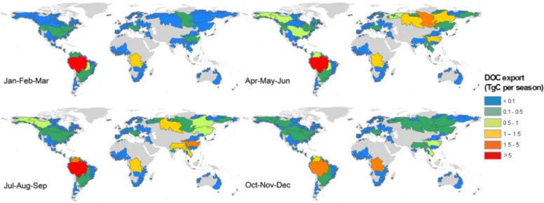
Fig. 7 reveals that the main contributor to the global riverine DOC
Fig. 2. Distribution of the different coefficients of determination for the
re-gression between observed and simulated daily DOC fluxes (TgC.yr−1) on the
two past decades for each of the 74 watersheds considered in the study. The
grey dashed line represents the limit (R2 = 0.35, p < 0.01) set in this paper.
The regression was not performed for the last watersheds on the graph as less than eight observations were available.
Fig. 3. Boxplots of the distribution of the returned parameters α and β of the
DOC equation estimated based on nonlinear least squares estimations. Black circles represent extreme values higher than the ninth decile of the boxplots. Coloured circles represent the selected rivers based on their respective Köppen- Geiger climate group. The selected rivers are representative of most of our dataset. (For interpretation of the references to color in this figure legend, the reader is referred to the web version of this article.)
Table 3
Indices and parameters of the DOC equation on different watersheds based on datasets in the 1990–2015 period. n represents the number of DOC observations used to calibrate the equation for each river. The p-values represent the sta-tistical validity of the regression. The percent of bias (PBIAS) describes how the simulations overestimate or underestimate observations if it is positive or ne-gative, respectively.
Rivers n Parameters Indices
α β R2 p-value PBIAS (%) Amazon 146 8.08 0.74 0.01 0.21 −0.02 Murray 420 22.2 0.02 0.40 < 0.001 −16.7 Yangtze 27 1.80 0.01 0.07 0.18 1.33 Rhône 68 2.40 0.27 0.14 0.002 −10.1 Save 557 5.12 0.15 0.46 < 0.001 0.86 Yenisei 199 15.8 1.39 0.70 < 0.001 0.58
Fig. 4. Comparison between observed and simulated yearly average DOC
concentrations (mg.L−1) on the two past decades for the 70 watersheds
exports is the Amazon River, with significant contributions of the Congo River and Asian rivers, particularly in Siberia during the spring freshet (April to June) and in South East Asia between July and September
(Fig. 8). A focus on both sides of the Atlantic Ocean shows that the
Amazon and the Congo rivers present different behaviours during the year (Fig. 8). The Amazon River seems to provide the first part of the DOC fluxes flowing into the Atlantic Ocean during the second trimester while the Congo River is taking over during the last trimester when the Amazon fluxes are decreasing. A videotape showing the seasonal fluc-tuations of daily DOC exports of each watershed considered in this paper is available as supplementary material and details these trends at a daily time step.
3.6. Global daily riverine DOC exports
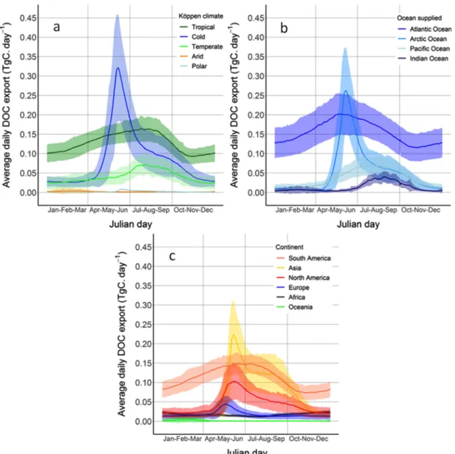
Fig. 9 shows the distribution of these daily global riverine exports
for each climatic group (Fig. 9a), each ocean supplied (Fig. 9b) and each continent (Fig. 9c). Concerning climate groups, the tropical and cold rivers represent the most important contributions to the DOC fluxes with different behaviours. The highest deliveries of tropical rivers occur in August with a peak near 0.16 TgC.day−1, but the daily fluxes remain high during the other part of the year. Cold streams ex-ports show a rapid increase in spring peaking at 0.32 TgC.day−1. The temperate rivers present an early period of high fluxes also lasting during a large part of the year. Still, their exports remain steady com-pared to tropical basins with daily deliveries going from 0.03 to 0.08
Fig. 5. Simulation of daily riverine DOC fluxes at the outlet of the selected river basins. The dots represent the observed DOC fluxes on days when concentrations
were sampled. The grey lines represent the predicted DOC fluxes calculated based on the observed daily discharges. Concerning the Yangtze River, we averaged daily discharge on the sampling period (2009–2011) based on available data in the 1982–2001 period.
Fig. 6. Regressions between the parameters of the DOC equation and environmental variables. The ratio between the soil organic carbon content and the amount of
precipitations explains the parameter α (left). The parameter β is related to the average annual air temperature (right). The top of the graphs shows the regressions between statistically determined values and predicted values of the settings.
Fig. 7. Global simulated riverine DOC fluxes (TgC.yr−1) exported to the oceans on the two past decades based on a dataset of 341 large river basins. 10° latitudinal zones and trimesters detail the DOC fluxes. The extrapolated DOC fluxes from exoreic catchments (dotted bars) are estimated based on the gap between the water
flows integrated into our study and the water flows of the global exoreic basins from The Global Runoff Data Centre (2014).
TgC.day−1. In contrast, the semi-arid rivers present some fluctuations between January and March, and the polar streams have higher fluxes in June. Though these exports are low compared to the other climate groups. In the same way, the most supplied oceans are the Atlantic Ocean and the Arctic Ocean while the most contributive continents are Asia and South America.
At last, we were able to extrapolate global riverine DOC fluxes to the oceans based on estimates of the water flows from exoreic watersheds
(The Global Runoff Data Centre, 2014). We compared the resulting
yearly fluxes with previous estimates (Table 4). The predicted total export of 0.13 Pg.yr−1 in this paper is lower than those of previous estimates, but the returned specific flux (1.7 t.km−2.yr−1) is in the range of most of the previous research (1.5–3.1 t.km−2.yr−1).
4. Discussion 4.1. Model validity
4.1.1. Validity of the DOC equation
The equation for riverine DOC exports proposed in this paper re-turned good results regarding the spatial and temporal variability. We showed a satisfactory fitting of our equation with the observations in
most of the 79 rivers studied (Fig. 2). This dataset shows large varia-bility in the characteristics of the basins regarding the size, the climate and the soil conditions. Moreover, simulated yearly average DOC con-centrations are in the range of observations (Fig. 4). The daily simu-lations produced by this generic model follow the observations trend
(Appendix A). Therefore, the yearly average simulated and observed
DOC concentrations are close while daily simulations for each catch-ment showed uncertainties. The processes were still well represented on the six selected watersheds (Fig. 5) where daily discharges were available for the whole sampling period. The DOC equation fitted the observations at a daily time step in the basins where the data demon-strated an evident variation in DOC concentrations between low and high-water flows (Appendix A). The basins where the equation fitted the observations with more difficulties and less accuracy are commonly those where the discharge is not the only variable explaining changes in DOC concentrations. The proposed equation generally represents the observations with a DOC concentration increase correlated with the discharge. However, it does not explain abrupt changes, as shown in
Appendix A for the Amazon River. These changes could be linked to
parameters not considered in this generic model or to changes in the hydrological functioning of the basin during specific years. As DOC is hard to collect and to measure, these abrupt changes could be due to
measurement errors. However, these variations could also be related to anthropogenic deliveries, which could produce different DOC con-centrations for the same discharge. As an example, we have shown that the model represents well the low-water DOC fluxes in the Amazon River but encounter difficulties to explain high-water fluxes (Fig. 5). The temporal dynamic returns accurate results at a daily time step for cold watersheds, such as the Yenisei River in Fig. 5. It also points out the weaknesses of the DOC equation for rivers with DOC concentrations varying independently of the discharge, e.g., the Amazon River in
Appendix A. In these rivers, our model simulates a constant DOC
con-centration. Therefore, this equation underlines the need to better measure and model daily water flows to obtain more accurate simu-lated DOC concentrations and fluxes. A lack of data or a bad re-presentation of the hydrological cycle in the dataset could explain the inability of our model to fit the observations. Some environmental conditions that are not considered in the equation so far could also justify this offset. As an example, wetlands could act as sources or sinks of organic carbon. This hypothesis can only be considered and checked by using process-based models which simulate the exchanges of carbon between the different components, as proposed by Nakayama (2017). However, the NICE-BGC model used in this paper has difficulties to fit the observed DOC fluxes for some large watersheds (Nakayama, 2017). Finally, this paper proposes a new way to estimate DOC fluxes to the oceans at the global scale. Indeed, when the fitting gave good results, the generic model can consider variations of DOC concentrations during the hydrological cycle, especially in cold and semi-arid rivers
(Appendix A). This specificity was not considered in previous empirical
equations and improved the estimations of riverine DOC fluxes to the oceans considerably. Thus, the fluxes calculated with the method de-tailed in this paper are closer to the estimates from Dai et al. (2012) based on observed data. When this generic model encountered diffi-culties to fit, it returned the yearly average DOC concentration in the river, which is close to what past studies proposed at the global scale.
4.1.2. Selection of environmental variables
The set of environmental variables used to find a suitable correla-tion with the parameters α and β was done by selecting variables in-fluencing DOC dynamics. The hypothesis of a link between Köppen- Geiger climate groups and DOC exports was made as Huang et al.
(2012) already proposed a model including Köppen-Geiger climate
groups. The watersheds in this study were classified as proposed by Mc
Mahon (1982). Concerning soil organic carbon content, it is the major
source of riverine DOC (Meybeck, 1993; Raymond and Bauer, 2001;
Schimel and Weintraub, 2003). Forest and coniferous forest coverage,
as well as Average Above Ground Biomass, are major sources of de-composed organic matter (McDowell and Likens, 1988; Laudon et al., 2011). Wetlands coverage is also strongly correlated with DOC pro-duction (Mitra et al., 2005). The relation between slope and DOC ex-ports were demonstrated at global scale (Ludwig et al., 1996). The slope is related to physical erosion as shown in the Modified Universal Soil Loss Equation (MUSLE; Williams, 1975), which was demonstrated in various cases (Sadeghi and Mizuyama, 2007). As for the slope, the precipitation is related to the physical erosion in the MUSLE equation
(Williams, 1975). Finally, a relation exists between the temperature and
the DOC concentrations (Raymond and Saiers, 2010). It is the first driver of microbial activity which is important in the organic matter decomposition and the formation of DOC (Wetzel, 1992; Vervier et al.,
1993; Schimel and Weintraub, 2003).
4.1.3. Environmental links with the parameters
The α parameter explains the potential of maximum DOC con-centration in the river. This potential is reached during the periods of discharge peaks. Then, the potential is linkable with the soil leaching. This leaching corresponds to the ratio between the organic carbon content in soils and the amount of precipitations, creating a dilution of the carbon pool. This leaching represents the primary source of DOC
Table 4 Exported riverine fluxes of DOC from exoreic watersheds on the two past decades. n represents the number of rivers on which the DOC fluxes were studied, and nextra is the number of streams used to extrapolate or refine the global DOC flux. This study Nakayama, 2017 Li et al., 2017 Dai et al., 2012 Seitzinger et al., 2010 Aitkenhead and McDowell, 2000 Ludwig et al., 1996 Meybeck, 1993 n (nextra ) 341 (423 ⁎ ) 153 263 118 (925) 5761 164 60 > 40 Estimated flux (and corrected flux; TgC.yr −1 ) 95.8 (131.6 ⁎ ) 461 240 170 (208) 164 362 205 199 Specific flux (t.km −2 .yr −1 ) 1.6 (1.7 ⁎ ) 4.7 2.8 2.1 (2.6) 1.5 3.1 1.9 2.0 ⁎based on the Interactive Database of the World's River Basins ( CEO Water Mandate, 2016 ) and The Global Runoff Data Centre (2014).
Houser, 2007). It is a central problem in the extrapolation of biogeo-chemical fluxes exported at a global scale. An improvement in the es-timates of global water flows to the oceans is necessary to better un-derstand the global dynamic of biogeochemical cycles.
Finally, our global riverine DOC flux highlights the fact that our dataset lacks daily discharge data on principal rivers in some parts of the world, such as the Indus River and the Salween River. Other rivers in India, Myanmar and Indonesia may play an essential role in the DOC export to the Indian Ocean and the global flux regarding their average discharge. Indeed, the extrapolation at global scale assumes that the 341 rivers used in this study are representative of each latitude interval they depict. A main progress to this model could be to sample and in-clude other main rivers to be more accurate in the exports enounced. We could also underline a lack of data for the Nile River and other rivers in North Africa, which could be main drivers of DOC exports in Africa as well as their respective climate group. A focus on the Arctic rivers is revealing that our flux in this region is in the range of
Seitzinger et al. (2010) value but does not fit the ones in previous
pa-pers (Appendix B). Our predictions for the Arctic watersheds could be evaluated as more accurate because we are least likely to underestimate or overestimate the impact of the spring freshet with daily time step fluxes.
4.3. Uncertainty analysis 4.3.1. Dataset quality
This study reviewed a consequent amount of data for DOC in rivers from various databases and studies (Tables 1 & 2). These data were hard to collect, and the protocols used to sample these concentrations are not similar. The errors linked to the sampling and the analyses are different for each watershed or each database. Plus, differences exist sometimes between 2 datasets for the same catchment as samplings were done during different decades in the last 30 years. The protocols and analyses methods evolved through the years, which could disrupt the optimi-zation of the DOC equation by using data from these different decades. Available daily riverine DOC concentrations are sparse and samples on more than one year are published and available only in few basins. Concerning environmental variables, the values found in this paper depends on the resolution of the datasets. The correlations demon-strated in this paper are relatively significant to highlight a pattern. Still, better datasets of DOC and more precise databases used to de-termine the environmental variables would help refine these results.
Plus, another consequent lack in this paper is that riverine DOC was not importantly studied compared to other nutrients. Many past studies focused on Total Organic Carbon without expressing the part of DOC in the global organic carbon balance. Nevertheless, recent research
Table 5
Influence of the deviations in the α parameter on the exported DOC fluxes of 8 large basins. The predicted α corresponds to the α determined with the
equa-tion of Fig. 6.
River Predicted α Exported
flux (TgC.yr−1) Statistically determined α Expected flux (TgC.yr−1) Difference (TgC.yr−1) Amazon 5.4 27.7 7.8 40.0 −12.3 Congo 5.5 5.4 16.7 16.4 −11.0 Lena 9.7 2.4 18.7 4.6 −2.2 Mississippi 5.8 1.4 3.6 0.9 0.5 Ob 15.8 2.8 10.2 1.8 1.0 Orinoco 5.4 5.4 6.1 6.1 −0.7 Yangtze 5.6 4.1 1.8 1.3 2.8 Yenisei 9.3 2.6 14.2 4.0 −1.4 Total −23.3
(Meybeck, 1993; Raymond and Bauer, 2001; Schimel and Weintraub,
2003). The β parameter of the equation is linked to the speed to reach the highest DOC concentrations. This parameter is negatively correlated to the average annual air temperature in the river basin (Fig. 6b). The more the watershed presents cold temperatures, the more time to reach the highest DOC concentrations in the river. The microbial activity could be underneath these correlations. It is the primary process at the origin of the DOC supply. Indeed, specific bacteria dependent on the temperature ensures the decomposition of the organic carbon in soils leading to DOC production (Balser and Wixon, 2009; Conant et al.,
2011).
4.2. DOC exports in watersheds
This study showed the capability of a generic model to represent DOC fluxes in various catchments around the world. Fig. 8 highlighted an offset between DOC deliveries of the Amazon River and the Congo River. This lag agrees with the seasonal discharge fluctuations of the two largest rivers of the world (Nkounkou, 1989). In the same way, the second trimester brings to light the effect of the spring freshet in Si-berian Rivers and the third trimester highlights the impact of the monsoon in South East Asia. Plus, Fig. 9 showed the large deliveries of DOC to the Atlantic Ocean as well as the strong influence of tropical and cold rivers to the global DOC balance. It highlights the impact of the Amazon and the Congo rivers presenting the highest daily discharges by far on Earth but also the short but intense influence of the spring fre-shets of the Siberian Rivers flowing into the Arctic Ocean on global fluxes.
The global riverine DOC export presented here is lower than those of previous works. Our estimate is based on 341 watersheds which represent a small part of the total number of exoreic basins (Seitzinger
et al., 2005; Dai et al., 2012) but they embody around 71% of the
freshwater flow from the main watersheds to the oceans. This dataset could be judged as representative of the total water flow and allow the extrapolation of our estimate on the exoreic zones. The main difference with most of the past research is that this study calculates the DOC exports with the daily average discharges and extrapolates the results based on the yearly average discharges of the remaining main water-sheds where daily DOC data are not available. In contrast, most of the previous works did extrapolations depending on drainage areas or are based on complex process-based models. Another advantage of this study is the inclusion of variability in DOC concentrations. On the one hand, some watersheds showed a simulated daily DOC concentration close to the average observed content. Still, the model returned daily variations in the DOC concentration, especially on Arctic watersheds
(Appendix A), a difference that most of the previous estimates did not
consider. Seitzinger et al. (2005), with the Global-NEWS model, and Dai
et al. (2012), with observed data, returned the closest results from ours.
It confirms that our predictions based on a generic model are close to reality. However, uncertainties remain in the calculations of the para-meters α and β. As an example, Table 5 compares the values of α de-termined statistically with the α calculated by the equation shown in
Fig. 6 for eight large rivers. The Amazon and the Congo rivers show
significant differences between the modelled and the expected DOC fluxes. A divergence near 25 TgC.yr−1 appears in these eight basins presenting the highest discharges in the world due to a bad re-presentation of α. Thus, we could expect a total DOC flux around 160 TgC.yr−1 by improving the correlations between the two parameters of the equations and the environmental variables. This corrected global flux is close to the estimates of Dai et al. (2012) and Seitzinger et al.
(2005).
Plus, uncertainties remain important in the estimation of global freshwater flows t o t he oceans (Oki and Kanae, 2006; Schlosser and
estimated this export in the past decade with various methods and models (Seitzinger et al., 2010; Dai et al., 2012; Li et al., 2017;
Nakayama, 2017). This paper brings a new generic model to complete
the ways of estimating this large flux useful for the estuaries and the oceanic food webs.
In this study, a database of daily discharges was created based on different datasets to predict the average daily DOC fluxes (Table 2). Similarly, the observed daily runoffs are not available for the same periods on the various rivers detailed in Table 2. We calculated the average interannual discharge at a daily time step in each catchment to represent its hydrological dynamics.
4.3.2. Uncertainty on the DOC equation parameters
Concerning the uncertainty analysis of the DOC equation para-meters, we tested the model with new values of soil organic carbon content, precipitations and air temperature by increasing and de-creasing them by five g.m−3 and 1 °C, respectively. It resulted in new values of α and β, as shown in Table 6. The model returns fluxes in the range of the base scenario between 129 and 137 TgC.day−1. Finally, the model seems stable and the parameters not very sensitive as errors in the estimation of these parameters produce uncertainties of less than 5%. However, the soil organic carbon content is the most sensitive variable because an offset between 5 and 7% for the parameter α produces an uncertainty close to 4% while similar errors in the amount of precipitations cause offsets around 2%. Changes in the parameter β upper than 10% induce uncertainties near 1%.
Furthermore, it appeared clear that the correlations between the parameters and the environmental variables could be improved, as shown for α in Table 5. By considering the influence of other en-vironmental variables on the two parameters, the relations used to determine them for each watershed should be more relevant.
4.4. Perspectives of use
In front of the uncertainties in the calculations of α and β (Fig. 6), collecting more observed DOC concentrations data for each basin seems essential. Plus, improving the way the organic carbon content in soils and the microbial activity influence the model is primordial to find a suitable set of parameters for each watershed and refine the river ex-ports at large scales. Previous works showed the global fluctuations of soil organic carbon stocks (Tian et al., 2015; Nakayama, 2020). These annual changes could be responsible for variations in DOC concentra-tions and their integration in our model should improve our global estimate. These enhancements are necessary to focus on the DOC dy-namics in rivers and on their effects on other biogeochemical cycles at the watershed scale e.g., in the denitrification process (Fabre et al.,
2020; Guilhen et al., 2020), and at global scale. Finally, these DOC
exports would help to assess contaminants transports as some elements such as mercury are known to be carried by DOC (Lavoie et al., 2019).
5. Conclusions
A new generic model is used to quantify daily DOC fluxes in rivers. The model depends on daily discharge and two parameters linked to the air temperature and the ratio of the organic carbon content in soils and the amount of precipitations. These environmental variables are related to the formation of DOC in rivers. We calibrated and validated this model with a large dataset of riverine DOC concentrations from various catchments. We used this equation to represent daily global DOC fluxes to the oceans. We found a total DOC export around 130 TgC.yr−1 for the past two decades in 341 main watersheds. This estimate is lower than in previous studies. The difference could be explained by un-certainties in the determination of the model parameters but also by the daily time step improving the estimation of DOC exports especially for rivers presenting quick transitions between high and low water flows such as Arctic rivers. The most top contributions are from tropical (49%) and cold (33%) watersheds delivering 82% of the exports mainly in the Atlantic and the Arctic oceans. This approach could be further introduced in hydrological modelling tools to study riverine DOC fluxes at global scale in a context of climate change.
Authors contributions
C.F., S.S. and J.M.S.P. designed and developed the model with the help of J.-L.P. C.F. performed and analyzed the modelling. C.F. wrote the paper with considerable contributions from S.S., J.M.S.P. and J.-L.P.
Additional information
This research did not receive any specific grant from funding agencies in the public, commercial, or not-for-profit sectors.
Declaration of Competing Interest
The authors declare that they have no known competing financial interests or personal relationships that could have appeared to influ-ence the work reported in this paper.
Acknowledgements
We do acknowledge Dr. Michel Meybeck, Dr. Sarah M. Stackpoole, Dr. Jens Hartmann and Dr. Stephan Kempe for their knowledge and sharing of available data and projects already done about riverine DOC exports. We do acknowledge Jérémy Guilhen for his various remarks in the analysis of the DOC equation. We thank the Global Runoff Data Center, the International Center for Water Resources and Global Change, the Observation Service SO HYBAM, the Arctic Great Rivers Observatory and the TOMCAR-Permafrost Project for the sharing of their data of DOC and daily discharge. This work was done during the French governmental PhD program of Clément Fabre.
Scenarios α (mg.L−1) β (mm.day−1) Resulting DOC export (TgC.day−1)
Base 7.8 ± 5.6 0.68 ± 0.96 131.6 ORGC +5 g.m−3 8.2 ± 5.7 (+5.1%) 136.1 (+3.4%) ORGC -5 g.m−3 7.3 ± 5.5 (−6.4%) 127.0 (−3.5%) PRECIP +5 mm 7.4 ± 4.9 (−5.1%) 129.4 (−1.7%) PRECIP -5 mm 8.3 ± 6.7 (+6.4%) 134.5 (+2.2%) TEMP +1 °C 0.59 ± 0.64 (−13.2%) 133.3 (+1.3%) TEMP -1 °C 0.90 ± 2.31 (+32.4%) 129.7 (−1.2%) Table 6
Appendix A. Fitting of the DOC model for the selected rivers. n represents the number of daily observations available for each watershed.
Appendix B. Comparison of DOC fluxes exported (TgC.yr-1) with past research. The corrected flux corresponds to adjustments made on the
eight large basins presented in Table 5.
Appendix C. Supplementary data
Supplementary data to this article can be found online at https://doi.org/10.1016/j.gloplacha.2020.103294.
References
United Nations Environment Programme, 2018. GEMStat database of the Global Environment Monitoring System for Freshwater (GEMS/Water) Programme. International Centre for Water Resources and Global Change, Koblenz Available upon request from GEMS/Water Data Centre. gemstat.org.
Ågren, A., Buffam, I., Berggren, M., Bishop, K., Jansson, M., Laudon, H., 2008. Dissolved
organic carbon characteristics in boreal streams in a forest-wetland gradient during the transition between winter and summer. J. Geophys. Res. 113. https://doi.org/10. 1029/2007JG000674.
Aitkenhead, J.A., McDowell, W.H., 2000. Soil C:N ratio as a predictor of annual riverine DOC flux at local and global scales. Glob. Biogeochem. Cycles 14, 127–138. https:// doi.org/10.1029/1999GB900083.
Aitkenhead, J.A., Hope, D., Billett, M.F., 1999. The relationship between dissolved or-ganic carbon in stream water and soil oror-ganic carbon pools at different spatial scales.
Hydrol. Process. 13, 1289–1302. https://doi.org/10.1002/(SICI)1099- 1085(19990615)13:8<1289::AID-HYP766>3.0.CO;2-M.
Araujo, M., Noriega, C., Lefèvre, N., 2014. Nutrients and carbon fluxes in the estuaries of major rivers flowing into the tropical Atlantic. Front. Mar. Sci. 1. https://doi.org/10. 3389/fmars.2014.00010.
Balakrishna, K., Probst, J.L., 2005. Organic carbon transport and C/N ratio variations in a large tropical river: Godavari as a case study, India. Biogeochemistry 73, 457–473. https://doi.org/10.1007/s10533-004-0879-2.
Balakrishna, K., Kumar, I.A., Srinikethan, G., Mugeraya, G., 2006. Natural and Anthropogenic Factors Controlling the Dissolved Organic Carbon Concentrations and Fluxes in a Large Tropical River, India. Environ. Monit. Assess. 122, 355–364. https://doi.org/10.1007/s10661-006-9188-7.
Balser, T.C., Wixon, D.L., 2009. Investigating biological control over soil carbon tem-perature sensitivity. Glob. Chang. Biol. 15, 2935–2949. https://doi.org/10.1111/j. 1365-2486.2009.01946.x.
Bao, H., Wu, Y., Zhang, J., 2015. Spatial and temporal variation of dissolved organic matter in the Changjiang: Fluvial transport and flux estimation: CHANGJIANG DOM. J. Geophys. Res. 120, 1870–1886. https://doi.org/10.1002/2015JG002948. Batjes, N.H., 2009. Harmonized soil profile data for applications at global and continental
scales: updates to the WISE database. Soil Use and Management 25 (2). https://doi. org/10.1111/j.1475-2743.2009.00202.x.
Bird, M.I., Robinson, R.A.J., Win Oo, N., Maung Aye, M., Lu, X.X., Higgitt, D.L., Swe, A., Tun, T., Lhaing Win, S., Sandar Aye, K., Mi Mi Win, K., Hoey, T.B., 2008. A pre-liminary estimate of organic carbon transport by the Ayeyarwady (Irrawaddy) and Thanlwin (Salween) Rivers of Myanmar. Quat. Int. 186, 113–122. https://doi.org/10. 1016/j.quaint.2007.08.003.
Birkett, C.M., Mason, I.M., 1995. A New Global Lakes Database for a Remote Sensing Program Studying Climatically Sensitive Large Lakes. J. Great Lakes Res. 21, 307–318. https://doi.org/10.1016/S0380-1330(95)71041-3.
Bowes, M.J., Armstrong, L.K., Wickham, H.D., Harman, S.A., Gozzard, E., Roberts, C., Scarlett, P.M., 2017. Weekly Water Quality Data from the River Thames and its Major Tributaries (2009–2013) [CEH Thames Initiative]. https://doi.org/10.5285/ e4c300b1-8bc3-4df2-b23a-e72e67eef2fd.
Brunet, F., Gaiero, D., Probst, J.L., Depetris, P.J., Gauthier Lafaye, F., Stille, P., 2005. δ 13 C tracing of dissolved inorganic carbon sources in Patagonian rivers (Argentina). Hydrol. Process. 19, 3321–3344. https://doi.org/10.1002/hyp.5973.
Centre for Ecology & Hydrology, 2020a. Environmental Information Data Centre. Centre for Ecology & Hydrology, 2020b. National River Flow Archive. CEO Water Mandate, 2016. Interactive Database of the World’s River Basins. Ciais, P., Sabine, C., Bala, G., Bopp, L., Brovkin, V., Canadell, J., Chhabra, A., Defries, R.,
Galloway, J., Heimann, M., Jones, C., Le Quéré, C., Myneni, R.B., Piao, S., Thomton, P., 2013. Carbon and Other Biogeochemical Cycles. In: Stocker, T.F., Qin, D., Plattner, G.-K., Tignor, M., Allen, S.K., Boschung, J. ... Midgley, P.M. (Eds.), Climate Change 2013: The Physical Science Basis. Contribution of Working Group I to the Fifth Assessment Report of the Intergovernmental Panel on Climate Change. Cambridge University Press, Cambridge, United Kingdom and New York, NY, USA. Cole, J.J., Prairie, Y.T., Caraco, N.F., McDowell, W.H., Tranvik, L.J., Striegl, R.G., Duarte,
C.M., Kortelainen, P., Downing, J.A., Middelburg, J.J., Melack, J., 2007. Plumbing the Global Carbon Cycle: Integrating Inland Waters into the Terrestrial Carbon Budget. Ecosystems 10, 172–185. https://doi.org/10.1007/s10021-006-9013-8. Conant, R.T., Ryan, M.G., Ågren, G.I., Birge, H.E., Davidson, E.A., Eliasson, P.E., Evans,
S.E., Frey, S.D., Giardina, C.P., Hopkins, F.M., Hyvönen, R., Kirschbaum, M.U.F., Lavallee, J.M., Leifeld, J., Parton, W.J., Megan Steinweg, J., Wallenstein, M.D., Wetterstedt, Martin, Bradford, M.A., 2011. Temperature and soil organic matter decomposition rates - synthesis of current knowledge and a way forward. Glob. Chang. Biol. 17, 3392–3404. https://doi.org/10.1111/j.1365-2486.2011.02496.x. Dai, M., Yin, Z., Meng, F., Liu, Q., Cai, W.-J., 2012. Spatial distribution of riverine DOC
inputs to the ocean: an updated global synthesis. Curr. Opin. Environ. Sustain. 4, 170–178. https://doi.org/10.1016/j.cosust.2012.03.003.
Déry, S.J., Hernandez-Henriquez, M.A., Burford, J.E., Wood, E.F., 2009. Observational Evidence of an Intensifying Hydrological Cycle in Northern Canada.
Drake, T.W., Raymond, P.A., Spencer, R.G.M., 2017. Terrestrial carbon inputs to inland waters: a current synthesis of estimates and uncertainty: Terrestrial carbon inputs to inland waters. Limnol. Oceanogr. Lett. 3, 132–142. https://doi.org/10.1002/lol2. 10055.
Drugge, L., Jonsson, K., Wörman, A., Ölander, B., 2003. Effect of Hydropower Regulation on the Transport of Metals and Nutrients in Lule River. (Uppsala).
European Commission, 2003. Global Land Cover 2000 Database.
Fabre, C., Sauvage, S., Tananaev, N., Noël, G.E., Teisserenc, R., Probst, J.L., Pérez, J.M.S., 2019. Assessment of sediment and organic carbon exports into the Arctic Ocean: the case of the Yenisei River basin. Water Res. 158, 118–135. https://doi.org/10.1016/j. watres.2019.04.018.
Fabre, C., Sauvage, S., Guilhen, J., Cakir, R., Gerino, M., Sánchez-Pérez, J.M., 2020. Daily denitrification rates in floodplains under contrasting pedo-climatic and anthro-pogenic contexts: modelling at the watershed scale. Biogeochemistry 149, 317–336. https://doi.org/10.1007/s10533-020-00677-4.
FAO, 2006. WRI Major Watersheds of the World Delineation. de Ferranti, J., Hormann, C., 2012. Digital elevation model. Zone 15-E.
Fick, S.E., Hijmans, R.J., 2017. WorldClim 2: new 1-km spatial resolution climate surfaces for global land areas: New climate Surfaces for Global Land areas. Int. J. Climatol. 37, 4302–4315. https://doi.org/10.1002/joc.5086.
Gao, Z., Tao, C., Shen, Y., Sun, W., Yi, Q., 2002. Riverine organic carbon in the Xijiang River (South China): seasonal variation in content and flux budget. Environ. Geol. 41, 826–832. https://doi.org/10.1007/s00254-001-0460-4.
Geeraert, N., Omengo, F.O., Borges, A.V., Govers, G., Bouillon, S., 2017. Shifts in the carbon dynamics in a tropical lowland river system (Tana River, Kenya) during
the scale of watershed influence on lakes and rivers. Ecol. Appl. 9, 1377–1390. https://doi.org/10.1890/1051-0761(1999)009[1377:DOCAAI]2.0.CO;2.
Gómez-Gutiérrez, A.I., Jover, E., Bodineau, L., Albaigés, J., Bayona, J.M., 2006. Organic contaminant loads into the Western Mediterranean Sea: Estimate of Ebro River in-puts. Chemosphere 65, 224–236. https://doi.org/10.1016/j.chemosphere.2006.02. 058.
Guilhen, J., Al Bitar, A., Sauvage, S., Parrens, M., Martinez, J.-M., Abril, G., Moreira- Turcq, P., Sanchez-Pérez, J.-M., 2020. Denitrification, carbon and nitrogen emissions over the Amazonianwetlands (preprint). Biogeochemistry. https://doi.org/10.5194/ bg-2020-3.
Hartmann, J., Lauerwald, R., Moosdorf, N., 2014. A brief overview of the GLObal RIver chemistry database, GLORICH. Procedia Earth Planet. Sci. 10, 23–27. https://doi. org/10.1016/j.proeps.2014.08.005.
Hengeveld, G.M., Gunia, K., Didion, M., Zudin, S., Clerkx, A.P.P.M., Schelhaas, M.J., 2015. Global 1-degree maps of forest area. Carbon Stocks Biomass 1950–2010. https://doi.org/10.3334/ORNLDAAC/1296.
Holmes, R.M., McClelland, J.W., Tank, S.E., Spencer, R.G.M., Shiklomanov, A.I., 2017. Arctic Great Rivers Observatory. (Water Quality Dataset).
Hope, D., Billett, M.F., Cresser, M.S., 1994. A review of the export of carbon in river water: Fluxes and processes. Environ. Pollut. 84, 301–324. https://doi.org/10.1016/ 0269-7491(94)90142-2.
Huang, T.-H., Fu, Y.-H., Pan, P.-Y., Chen, C.-T.A., 2012. Fluvial carbon fluxes in tropical rivers. Curr. Opin. Environ. Sustain. 4, 162–169. https://doi.org/10.1016/j.cosust. 2012.02.004.
Ittekkot, V., Arain, R., 1986. Nature of particulate organic matter in the River Indus, Pakistan. Geochim. Cosmochim. Acta 50, 1643–1653. https://doi.org/10.1016/ 0016-7037(86)90127-4.
Ittekkot, V., Laane, R.W.P.M., 1991. Fate of Riverine Particulate Organic Matter, in: Biogeochemistry of Major World Rivers. SCOPE, pp. 356.
Johnson, K.A., Goody, R.S., 2011. The Original Michaelis constant: translation of the 1913 Michaelis–Menten Paper. Biochemistry 50, 8264–8269. https://doi.org/10. 1021/bi201284u.
Kicklighter, D.W., Hayes, D.J., McClelland, J.W., Peterson, B.J., McGuire, A.D., Melillo, J.M., 2013. Insights and issues with simulating terrestrial DOC loading of Arctic river networks. Ecol. Appl. 23, 1817–1836. https://doi.org/10.1890/11-1050.1. Laudon, H., Berggren, M., Ågren, A., Buffam, I., Bishop, K., Grabs, T., Jansson, M., Köhler,
S., 2011. Patterns and Dynamics of Dissolved Organic Carbon (DOC) in Boreal Streams: the Role of Processes, Connectivity, and Scaling. Ecosystems 14, 880–893. https://doi.org/10.1007/s10021-011-9452-8.
Lavoie, R.A., Amyot, M., Lapierre, J., 2019. Global meta-analysis on the relationship between mercury and dissolved organic carbon in freshwater environments. J. Geophys. Res. 124, 1508–1523. https://doi.org/10.1029/2018JG004896. Le, T.P.Q., Dao, V.N., Rochelle-Newall, E., Garnier, J., Lu, X., Billen, G., Duong, T.T., Ho,
C.T., Etcheber, H., Nguyen, T.M.H., Nguyen, T.B.N., Nguyen, B.T., Da Le, N., Pham, Q.L., 2017. Total organic carbon fluxes of the Red River system (Vietnam): TOC fluxes of the Red River. Earth Surf. Process. Landf. 42, 1329–1341. https://doi.org/ 10.1002/esp.4107.
Lehner, B., Döll, P., 2004. Development and validation of a global database of lakes, reservoirs and wetlands. J. Hydrol. 296, 1–22. https://doi.org/10.1016/j.jhydrol. 2004.03.028.
Lesack, L.F.W., Hecky, R.E., Melack, J.M., 1984. Transport of carbon, nitrogen, phos-phorus, and major solutes in the Gambia River, West Africa. Limnol. Oceanogr. 29, 816–830. https://doi.org/10.4319/lo.1984.29.4.0816.
Li, M., Peng, C., Wang, M., Xue, W., Zhang, K., Wang, K., Shi, G., Zhu, Q., 2017. The carbon flux of global rivers: a re-evaluation of amount and spatial patterns. Ecol. Indic. 80, 40–51. https://doi.org/10.1016/j.ecolind.2017.04.049.
Lu, J.Z., Zhang, L., Cui, X.L., Zhang, P., Chen, X.L., Sauvage, S., Sanchez-Perez, J.M., 2019. Assessing the climate forecast system reanalysis weather data-driven hydro-logical model for the Yangtze River basin in China. Appl. Ecol. Environ. Res. 17, 3615–3632. https://doi.org/10.15666/aeer/1702_36153632.
Ludwig, W., Probst, J.-L., Kempe, S., 1996. Predicting the oceanic input of organic carbon by continental erosion. Glob. Biogeochem. Cycles 10, 23–41. https://doi.org/10. 1029/95GB02925.
Malcolm, R.L., Durum, W.H., 1976. Organic Carbon and Nitrogen Concentrations and Annual Organic Carbon Load of Six Selected Rivers of the United States. https://doi. org/10.3133/wsp1817F.
Mantoura, R.F.C., Woodward, E.M.S., 1983. Conservative behaviour of riverine dissolved organic carbon in the Severn Estuary: chemical and geochemical implications. Geochim. Cosmochim. Acta 47, 1293–1309. https://doi.org/10.1016/0016-7037(83) 90069-8.
Martins, O., Probst, J.-L., 1991. Biogeochemistry of Major African Rivers: Carbon and Mineral Transport - chapter 6. In: Biogeochemistry of Major World Rivers. John Wiley & Sons, pp. 127–155 (SCOPE; 42).
Mc Mahon, T.A., 1982. Hydrological Characteristics of Selected Rivers of the World. McDowell, W.H., Likens, G.E., 1988. Origin, Composition, and Flux of Dissolved Organic
Carbon in the Hubbard Brook Valley. Ecol. Monogr. 58, 177–195. https://doi.org/10. 2307/2937024.
Mekong River Commission, 2020. Daily observation and forecast of the Mekong River. Meybeck, M., 1993. Riverine transport of atmospheric carbon: sources, global typology
and budget. Water Air Soil Pollut. 70, 443–463. https://doi.org/10.1007/ BF01105015.
Meybeck, M., Vörösmarty, C.J., 1999. Global transfer of carbon by rivers. Global Change Newsl. 37, 18–19.
flooded and non-flooded conditions. Biogeochemistry 132, 141–163. https://doi.org/ 10.1007/s10533-017-0292-2.