Département de Géomatique appliquée faculté des Lettres et sciences humaines
Université de Sherbrooke
Explorîng Snow Information Content of Interferometric
SAR Data
Exploration du contenu en information de l’interférométrie RSO lié à la neige
Ah Esmaeily Gazkoliaui
Thesis submitted in fulfihiment of the requirements for the degree of Doctor of Phîlosophy (Ph.D.) in Remote Sensing
Thèse présentée pour l’obtention du grade de Philosophiae Doctor (Ph.D.) en Télédétection
© Ail Esmaeily Gazkohani, 200$
fN
Explorïng Snow lnformatïon Content of Interferometric SAR Data
Exploration du contenu en information de l’interférométrie RSO lié à la neige
Ail Esmaeïiy Gazkohani
Members of jury:
Cette thèse a été évaluée par un jury composé des personnes suivantes
Hardy B. Granberg
Directeur de recherche : (Département de Géomatique appliquée,Université de Sherbrooke) Q. Hugh J. Gwyn
Codirecteur de recherche : (Département de Géornatiqueappliquée, Université de Sherbrooke) Dong-Chen 11e
Membres dujury: (Département de Géomatique appliquée, Université de Sherbrooke) Matti Leppranta
Membres du jury: (Departrnent ofPhysics, University ofHelsinki, Finland) Bruce G. Thom
tftci’t pwte &we anti
tIei’t
patienceThe objective of this research is to explore the information content of repeat-pass cross-track Interferornetric SAR (InSAR) with regard to snow, in particular Snow Water Equivalent (SWE) and snow depth. The study is an outgrowth ofearher snow cover modeling and radar interferometry experiments at Schefferville, Quebec, Canada and elsewhere which has shown that for reasons of loss of coherence repeat-pass InSAR is not useful for the purpose of snow cover mapping, even when used in differential InSAR mode. Repeat-pass cross-track InSAR would overcome this problem.
As at radar wavelengths dry snow is transparent, the main reftection is at the snow/ground interface. The high refractive index of ice creates a phasedelay which is linearly reÏated to the water equivalent of the snow pack. When wet, the snow surface is the main reflector, aid this enables measurement of snow depth. Algorithms areelaborated accordingly.
Field experiments were conducted at two sites and employ two different types of digital elevation models (DEM) produced by means of cross track InSAR. One was from the Shuttie Radar Topography Mission digital elevation model (SRTM DEM), ftown in February 2000. It was cornpared to the photogrammetrically produced Canadian Digital Elevation Model (CDEM) to examine snow-related effects at a site near Schefferville, where snow conditions are well known from haif a century of snow and permafrost research. The second type of DEM was produced by means of airborne cross track InSAR (TOPSAR). Several missions were flown for this purpose in both summer and winterconditions during NA$A’s CoÏd Land Processes Experiment (CLPX) in Colorado, USA. Differences between these DEM’s were compared to snow conditions that were well documented during the CLPX field carnpaigns. The resuits are not straightforward. As a resuit of automated correction routines employed in both SRTM and ALRSAR DEM extraction, the snow cover signal is contaminated. Fitting InSAR DEM’s to known topography distorts the snow information, just as the snow cover distorts the topographic information. The analysis is therefore rnostly qualitative, focusing on particular terrain situations.
At ScheffervilÏe, where the SRTM was adjusted to Iuown lake levels, the expected dry-snow signal is seen near such lakes. Mine pits and waste dumps flot included in the CDEM are depicted and there is also a strong signal related to the spatial variations in SVŒ produced by wind redistribution of snow near lakes and on the alpinetundra.
In Colorado, cross-sections across ploughed roads support the hypothesis that in dry snow the SWE is measurable by differential InSAR. They also support the hypothesis that snow depth may be measured when the snow cover is wet. Difference maps were also extracted for a 1
km2 Intensive Study Area (ISA) for which intensive ground truth was available. Initial
comparison between estimated and observed snow properties yielded low coneÏations which improved after stratification ofthe data set.
In conclusion, the study shows that snow-related signals are measurable. For operational applications satellite-borne cross-track InSAR would benecessary. The processing needs to be snow-specific with appropriate filtering routines to account for influences by terrain factors other than snow.
Key words: Interferometry, InSAR, Snow Water Equivalent, SWE, Snow depth, Dry Snow, Wet Snow, AIRSAR, CLPX, SRTM, Schefferville.
L’objectif de cette recherche consiste à explorer le contenu en information de l’interférornétrie radar (InSAR) à passage multiple avec deux antennes, lié à la neige, en particulier l’équivalent en eau et sa profondeur. L’étude fait suite aux expériences de modélisation de couvert nival et d’interférométrie radar à Schefferville, Québec, Canada et d’autre endroit. Ces dernières montrent qu’à cause de perte de cohérence, l’interférométrie à passage multiple n’est pas convenable pour la détection de la neige, même dans le mode de InSAR Différentielle. InSAR
à passage multiple avec deux antennes devrait résoudre le problème.
Puisque la neige sèche est transparente pour le radar, la rétrodiffusion principale se produit à l’interface de neige/sol. Le haut indice de réfraction de la glace génère un déphasage qui est une approximation à l’équivalent en eau du couvert neigeux. Quand la neige est humide, sa surface est le réflecteur principal et ceci permet la mesure de profondeur de la neige. En conséquence, des algorithmes sont développés.
Les travaux expérimentaux ont été appliqués pour deux sites en utilisant deux types de modèle numérique d’altitude (MNA) générés par InSAR avec deux antennes. Le premier venait de données du Shuttie Radar Topography Mission (SRTM) qui a fait le tour de Globe en février 2000. Ceci a été comparé avec le MNA canadien généré en moyen photogrammétrie pour examiner les effets de la neige sur le radar dans un site près de Schefferville, où les conditions de neige est bien connus d’un demie centenaire de recherche sur la neige et pergélisol. Le deuxième type de MNA a été généré en utilisant les données InSAR aéroportées avec deux antennes (TOPSAR). Pour cette fin, plusieurs missions ont été planifiées en été et en hiver dans le cadre de projet Cold Land Processes Experiment (CLPX) au Colorado (ÉU). Les différences entre ces MNA ont été comparées avec les conditions de la neige qui ont été bien documentées pendant la campagne du terrain de projet CLPX.
Les résultats n’ont pas permis de valider la méthode de manière définitive. En raison des routines de corrections automatisées utilisées dans l’extraction de DEM des données SRTM et ATRSAR, le signal lié à la neige est bruité. L’ajustement de DEM d’InSAR à la topographie connue affecte l’information de neige, de la même manière que la neige affecte l’information topographique. L’analyse est donc qualitative, se concentrant sur des situations particulières de terrain.
À
Schefferville, où les MNA de SRTM ont été ajustés sur les niveaux connus des lacs, le signal prévu de la neige sèche est observé près de tels lacs. Des puits de mine et les décharges de rebut qui ne sont pas inclus dans le DEM Canadien sont détectés et il y a également un signal fort lié aux variations spatiales de l’équivalent en eau produit par la redistribution de la neige par le vent sur la toundra.Au Colorado, les profils transversaux des routes déneigées soutiennent l’hypothèse que l’équivalent en eau pour la neige sèche est mesurable par InSAR différentiel. Elles soutiennent également l’hypothèse que la profondeur de neige peut être mesurée quand la neige est humide. Des cartes de différence ont été également extraites pour un site d’étude I km2 (Intensive Study Area - ISA) pour lequel la vérité du terrain était disponible de façon
rapporté de faibles corrélations qui ont été améliorés après la stratification des données.
En conclusion, l’étude prouve que les signaux liés à la neige sont mesurables. Pour des applications opérationnelles l’approche de l’interférométrie radar avec deux antennes par moyen satellitaire est nécessaire. Le traitement doit être conçu pour la neige avec des routines de filtrage appropriées pour expliquer des influences par des facteurs de terrain autres que la neige.
Mots clefs Interférométrie, kSAR, Équivalent en eau, Profondeur de neige, Neige sèche, Neige humide, AIRSAR, CLPX
Table of contents I
List of figures iii
List of tables vii
Acronyms vIIi
Acknowledgments ix
1 INTRODUCTION 1
1.1 Background to the study 1
1.2 Objectives 5 1.2.1 General objective 5 1.2.2 Specific objectives 6 1.3 Hypotheses 6 1.4 Thesis outiine 6 1.5 Claim to originality 7
2 SNOW PROPERTIES AND CHARACTERISTICS 8
2.1 Snowcover $
2.2 Snow spatial variability and distribution 10
2.2.1 Snow accumulation 10
2.2.2 Effect ot topography onsnow coverdistribution 10
2.2.3 Effect of vegetation 11
2.2.4 Effectofwind 12
2.3 Mictowave interactions and dielectric properties ofsnow 12
3 INTERFEROMETRIC SAR 19
3.1 Theory 19
3.1.1 Differential lnterferometry 22
3.1.2 Errors and limitations ofInSAR 24
3.2 The influence of wet and dry snow on InSAR DEM’s 27
3.2.1 Dry condition 27
3.2.2 Wet condition 31
3.3 Theoretical analysis 32
3.5 Conclusion of theoretical research.3$
4 METHODOLOGY 39
4.1 Introduction 39
4.2 Schefferville study area and data 39
4.3 Data 41
4.4 Colorado study areas and data 41
4.4.1 Characteristics of Meso-ceIl Study Areas (MSA) 43
4.4.2 Characteristics of Intensive Study Areas (ISA) 49
4.4.3 AIRSAR data 50 4.4.4 Ground data 52 4.5 Method of analysis 56 4.5.1 SRTM InSAR data 56 4.5.2 CLPX InSAR data 56 4.5.3 Elevation correction 5$
4.5.4 Interactive image georeferencing 5$
4.5.5 Misfit between TOPSAR DEM’s 60
4.5.6 Snow spatial variability 63
4.5.7 SWE and snow depth estimation 63
4.5.8 Data ntegration 63
5 RESULTS AND DISCUSSION 65
5.1 Results at Schefferville 65
5.2 Results from Colorado 6$
5.3 Integration of remote sensing and field data 76
5.4 SWE and depth estimation 77
5.5 The nature of the snow depth and water equivalentsignais 81
5.5.1 Snow water equivalent $2
5.5.2 Snow depth 85
6 CONCLUSIONS 90
7 REFERENCES 92
8 APPENDIX1 102
List of Figures
Figure 1: Three examples of coherence images of repeat-passinterferornetry with 3 days interval, calculated from ERS-1 parent images, (a) January 9 and 12, (b) January 12 and 15,
(e) February 14 and 17 (Images provided by Vachon etaÏ., 1995) 3
Figure 2: (a) RADARSAT coherence image from pairimage ofDecernber 1 and 25, 1996, (b) RADARSAT coherence image from pair image ofFebruary 2$ and Mardi 24, 1997, (e) Part of permafrost map produced by 10CC in 1972-74 (modifiedafter Granberg and Vachon,
199$) 4
figure 3: The penetration depth of snow decreases rapidlywith increasing liquid water
content, especiaÏly in the immediate vicinity ofLw= O (rnodified after Ulaby et aL, 1986).... 15
figure 4: Real part of tic dielectric constant of dry snow as a ftmction ofthe density of dry snow relative to water (modified after Tiuri et aÏ., 1984) 15 Figure 5: The unit ceil of a grain cluster showing a liquid vein at the three-grain junction and three liquid fluets at grain boundaries (after CoÏbeck, 1980) 16 Figure 6: a- The spectral variation of the permittivity ofwet snow with snow wetness as a parameter; b - The spectral variation ofthe loss factor ofwet snow with snow
wetness as a parameter. The curves are based on the rnodifiecÏ Debye-Ïikemodel (afler Haïlikainen et aï.,
1986) 17
Figure 7: Geometry ofrepeat-pass InSAR 21
Figure 8: Modeled interferogram with black unes denoting knownfault unes and coloured
fringes related to changes in surface elevation 23
figure 9: Standard deviation ofthe phase estirnate as a functionofcoherence and number of
independent samples L (after Barnler and Hart 1998) 25
Figure 10: Refraction change due to difference in dielectricproperties between air and snow28 Figure 11: Variation of interferornetric phase difference versus sensor incidence angle. The color curves represent the snow pack depth variation (from 5 to 100 cm) having a densïty of
0.3gc& 33
Figure 12: Variation ofinterferometric phase difference versus sensor incidence angle. The color curves represent the snow pack depth variation (from 5 to 100 cm) having a density of
0.4gcrn3 33
Figure 13: Variation of interferometric phase difference versus sensor incidence angle. The color curves represent the snow pack depth variation(from5 to 100 cm) having a density of
Figuie 14: InSAR phase difference variation versusthe changes in Snow Water Equivalent (SWE) having a density of 0.3 g cm3. The plotted unes represent the sensor incidence angle
with highlight on ERS satellites incidence angle of23° 35
figure 15: InSAR phase difference variation versus the changes in Snow Water Equivaient (SWE) having a density of 0.4 g cm3. The plotted lines represent the sensor incidence angle
with highuight on ERS satellites incidence angle of 23° 35
Figure 16: InSAR phase difference variation versus the changes in Snow Water Equivalent (SWE) having a density of 0.5 g cm3. The plotted unes represent the sensor incidence angle
with highlight on ERS satellites incidence angle of23° 36
Figure 17: Schefferville study area 40
figure 18: Schematic diagram of the nested study areas for the Cold Land Processes Field
Experiment 42
Figure 19: The three 25 km x 25 km study areas, and the nested Intensive Study Areasare
shown with red boundaries 43
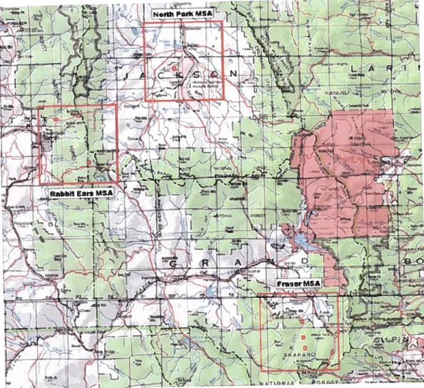
Figure 20: The 25 km x 25 km North Park Study Areaboundaries are shown in red. Nested within the area are three 1 km x 1 km Intensive StudyAreas: Potter Creek ISA, flhinois River ISA, and Michigan River ISA (modified after NASAweb site) 45 Figure 21: The 25 km x 25 km Rabbit Ears Study Areaboundaries are shown in red. Nested within the area are three 1 km x 1 km Intensive Study Areas: Buffalo Pass ISA, Spring Creek
ISA, and Walton Creek ISA (modified after NASA web site) 47
Figure 22: The 25 km x 25 km Fraser Study Area boundaries are shown in red. Nested within the area are three 1 km x 1 km Intensive Study Areas: St. Louis Creek ISA, Fool Creek ISA,
and Alpine ISA (modified after NASA web site) 48
figure 23: Backscatter image of Rabbit Ears MSA acquired byAIRSAR instrument on
Febniary21st 2002 (tsl6O6c.vvi2) 51
Figure 24: DEM image ofRabbit Ears MSA acquired byAIRSAR instrument on February
21st, 2002 (tsl6O6c.demi2) 52
Figure 25: Map showing snow sample locations for each ISA. Red diamonds are first day sampling (snow depth, snow wetness, and snow surfacerouglrness). The blue squares are sampling on day 2 (snow pits, sec next figure) and green diarnonds are some special sampling
for period of 2003 54
Figure 26: Locations of CLPX Snow Pits within each Intensive Study Area 55
Figtire 28: Topographic map ofWalton Creek area in 1/13 000 scale dated 1956 (modified
after www.terraserver.com) 59
Figure 29: Aerial photography of Walton Creek areadated 1999 (modified after
www.tenaserver.corn) 60
Figure 30: Illustration ofthe effect of snow cover onperceived ground topography using differential interferometry using SRTM and CanadianDEM for Schefferville region (Québec)
66
Figure 31: Difference map and corresponding topographic rnap of the Lac Vacher area 67 figure 32: Difference map and coiiesponding topographiemap of mine pits 67 Figure 33: Difference rnap and topographie map ofthe east-center parts ofthe study area 68 Figure 34: DEMs and Backscatter extractions from Walton CreekISA. Extracted from: A,
Febntary; B, March and C, September acquisitions 69
Figure 35: Sampling profile in the Walton Creek ISA September DEM’s 70 Figure 36: Altitude verification of 1294 pixels ofthetwo different AIRSAR images on the
sameday 70
Figure 37: Coffelation of the altitude profiles for two $eptember erossed images ofWalton
Creek ISA 71
Figure 38: Validation of altitude correlation for 200 samples of Walton Creek ISA 72 figure 39: The variation of altitude ofAIRSAR data overa road for (IOPY and BG2) 73 Figure 40: The variation of altitude ofAIRSAR data overa road for (IOP2 and BG2) 73 Figure 41: Altitude eolTelation for two crossed images (Feb & Sep) ofWalton Creek ISA 74 Figure 42: Altitude correlation for two crossed images (Mar & Sep) ofWalton Creek ISA 74
Figure 43: Difference Map of September and February 75
Figure 44: Difference Map of March and September 75
Figure 45: Allocating the density by distance 76
Figure 46: Joining the snow density and snow depth data 76
Figure 47: Joining SWE ofAIRSAR data to shape file of ground data 77 figure 48: Distribution rnap of SWE differences based on comparison of remotely sensed
Figure 49: Distribution map of Snow Depth error .72 Figure 50: The location of transverse profiles in Rabbit Ears MSA 79 Figure 51: The location of transversal profiles in Fraser M$A 79
Figure 52: Profile 1 near Rabbit Ears 20
Figure 53: Distribution of ground tntth SWE $2
Figure 54: Distribution ofmeasured $WE based on InSAR $2
Figure 55: Distribution of$WE differences (ground trnth and InSAR) $3 Figure 56: Evaluating the measured and estimated SWE correlation 23 Figure 57: Applied mask on the Walton ISA to separate higher altitude (outside of green & inside of yellow zones) from lower altitudes in four sectionsA, 3, C and D $4 Figure 52: SWE correlations of low altitude points of 4 sections of Walton ISA $5 Figure 59: Statistical resuits ofground tnith snow deptli 86 Figure 60: Statistical resuits ofrneasured snow depth byInSAR 86 Figure 61: Statistical resuits of snow depth differences (ground truth and InSAR) 86
Figure 62: Measured vs. estimated snow depth 87
List of Tables
Table 1: Coordinates for corners of each MSA, givenfirst in Iatitude/longitude, then in UTM.
The WGS$4 datum is used foi- ail coordinates 44
Table 2: Characteristics ofthe Meso-ceil study areas, the general physiographic regimes they are considered to represent, and the approximate percentage of global, seasonaÏly snow
covered areas having these characteristics 44
Table 3: Location and characteristics of ISA. UTMcoordinates are given for upper left (UL)
and lower right (LR) corners 49
Table 4: Different kind of imagery produced by ALRSARdata 51
Table 5: AIRSAR ftight unes and length 52
Acronyms
AIRSAR Airbome Synthetic Aperture Radar
BG Bare Ground
CARTEL Centre d’Applications et de Recherches en Télédétection CDEM Canadian Digital Elevation Model
CLPX Cold Land Processes Experiment
DEM Digital Elevation Model
Diff-Map Difference Map
DInSAR DifferentiaÏ Interferornetry Synthetic Aperture Radar
DN Digital Number
ESA European Space Agency
GCP Ground Control Points
GIS Geographic Information System
InSAR Interferometry Synthetic Aperture Radar
10CC Iron Ore Company of Canada
IOP Intensive Observation Period
ISA Intensive Study Areas
JPL Jet Propulsion Laboratory
MSA Meso-celi Study Areas
NSIDC National Snow and 1cc Data Center SDT Schefferville Digital Transect SRTM Shuttie Radar Topographic Mission
SWE Snow Water Equivalent
TOPSAR Topographic Synthetic Aperture Radar
UTM Universal Transverse Mercator
Acknowledgments
I would like to express my gratitude to mysupervisor, Hardy B. Granberg, who suggested this
topic for investigation, and whose interesting discussion, insightful critique, and final editing ofthe thesis were instrumental to the successfuÏ compÏetionof this project.
I would especially like to express my deep gratitude to rny co-supervisor
Q.
Hugh I. Gwyn forhis valuable scientific advice, his guidance, and his constant availability by Internet, even when he was on the other side of the world.
I greatly appreciate the helpful discussion and suggestion of Marcel Laperle, as well as the aid
of various professors, colleagues and personnel at the Centre d’Applications et de Recherches en Télédétection (CARTEL) at the Université de Sherbrooke.
I want to thank Professor Ferdinand Bonn, who is no longer among us. whom I had the great
occasion to benefit of his presence and his reach of scientificknowledge (May God bless him).
My particular thanks go to my family; my wife Maryam, my sons Pouria and Parham and rny beloved parents whose prayers for me are my main fortune.
My final acknowledgments are dedicated to Ministry of Research and Technology of the Islamic Republic of Iran for granting me a research scholarship.
AIR$AR images and Field data were provided by NASA, Jet Propulsion Laboratory (JPL) and National Snow and Ice Data Center (NSIDC) of United States of America, I thank them respectively.
&4Øw
1
INTRODUCTION
1.1 Background to the study
Snow cover plays a significant foie in the energy and water budgets of the Earth on a variety of spatial and temporal scales. The storage of large arnounts of fresh water in seasonal snow covers is a critical element of the Earth’s hydrologie cycle. The Snow Water Equivalent (SWE) determines how rnuch liquid water per unit area will result in case where the snow cover is cornpletely melted and it is, therefore, an important quantity in snow-meh ninoff prediction for hydro-power and agricultural purposes.
Seasonai snow covers through their influence on land surface albedo, radiation balance and boundary layer stability, have profound effects onweather patterns over large areas.
On average, over 60% of the northem hemisphere land surface and over 30% of the Earth’s land surface has seasonal snow (Robinson, et al., 1993). In many mountainous regions, snowfall is a substantial part ofthe overail precipitation(Serreze et al., 2000), and snowrnelt is a major source of the total amiuaÏ stream ftow. While water from snow meit can be a vitally important natural resource, it can also become an environrnental hazard when rapid melting of
The properties ofthe slow cover are ofinterest on a local scale. At Schefferville(55°N, 67°W) the close corTelation between local snow depth variations and the distribution of permafrost (Annersten, 1966) sparked intensive research on the spatial variations in snow accumulation (Thom, 1969; Thom and Granberg, 1970) which led to the development of methods to rnap snow depth using air photo sequences ftown during spring meÏt (Granberg, 1972; 1973; NichoÏson, 1975). It also lcd to the development of an early Geographic Information System
(GIS) technique to reconstruct past snow covers for mines already under excavation (Granberg, 1972; 1973). The vast spatial database on snow cover characteristics thus generated together with Ïong-term snow cover monitoring by students and staff of the McGiIl Sub-Arctic Research Station for hydrologic and otherpurposes (Adams et cil., 1996; Nicholson and Thom, 1973; Nicholson and Granberg, 1973) made Schefferville the logical choice as principal field site for snow cover modeling experirnents sponsored by the Department of National Defence. As part ofthese studies the ScheffervilleDigital Transect was established in an area NW of Schefferville (Granberg and Irwin, 1991). The modeling research further lcd to exploration of radar as tool for terrain mapping (Granberg, 1994; Granberg et al., 1994) and snow model validation which brought exploratory experiments by Vachon et aï. (1995) to the SDT. h these experiments ERS-1 in 3-day orbit over the SDT provided parent images for repeat-pass interferornetric processing over varying time intervals extensib]e from December 25, 1993 to March 28, 1994. figure 1 shows examples of coherence images from this data set.
The InSAR data created from images with three-day intervaïs showed that for the exposed rock and alpine tundra, the scene coherence is always high but for other surface cover types, the coherence is more variable. In the two first images (left) snow fail between the two satellite overpasses created a loss of coherence while in the right one there was no snow fali between the overpasses.
Subsequent analyses (Fisette, 1999) demonstrated the existence of a strong, snow-related topographic signal, but it also demonstrated that repeat-pass InSAR is not suited for SWE mapping. For such mapping, cross-track interferometry is required. Other research (Côté, 1998) demonstrated that interferometric coherence is a useful and unique tool to study lake ice forming processes, in particular internai ftooding ofthe snow cover on lakes.
Using a different data source (RADARSAT-1), Granberg and Vachon (1998) dernonstrated that die spatial distribution of discoutinuous permafrost can be rnapped with good accuracy using InSAR coherence.
(c)
figure 1: Three examples ofcoherence images ofrepeat-pass interferometry with 3 days interval, caÏcuÏated from ERS-1 parent images, (a) January9 and 12, (b) January 12 and 15,
(c) February 14 and 17 (Images provided by Vachon etctl., 1995)
Over the 24-day orbit interval of RADARSAT-1 snow accumulation may cause loss of coherence, except in areas where wind continually sweeps away the snow that fails. As previous researci has shown, such parts ofthe terrain lose their protective snow cover, causing the average annual ground temperature to approach that of the air, which at Schefferville is about -5 oc (Nicholson and Granberg, 1973; Granberg et al., 1994). The interferometrically produced maps of the zones of shallow sriow (Figures. 2a, b) closeÏy match a map of permafrost (Figure 2c) produced by the Iron Ore company of Canada (10CC) using air photo interpretation, ground probing and geological trenching data (Granberg and Vachon, 1998).
The research at Schefferville forms the background to the current study. However, although the research at Schefferville took the Iead in this field, research on snow cover applications of radar interferornetry has progressed elsewhere also. Shi et aÏ., (1997) had also attempted mapping the snow cover using repeat-pass InSAR and Strozzi et al. (1999) had found repeat pass InSAR coherence useful in the mapping ofwet snow.
Figure 2: (a) RADARSAT coherence image frompair image ofDecember 1 and 25, 1996, (b) RADARSAT coherence image from pair imageof February 28 and March 24, 1997, (e) Part
of permafrost map produced by 10CC in 1972-74 (modified after Granberg and Vachon, 199$), Areas swep the snow bu the wind retaincoherence (white) while other parts lose
coherence due to snow accumulation
Granberg and Vachon (199$) suggested that the refraction of microwaves by dry snow should produce a phase-shifi which is linearly related to the SWE. Guneriussen et aÏ. (2001) elaborated this relationship further, and calculated that at the nominal ERS satellite incidence angle (&j=23°):
=2ki(0.$7SWE) (1)
Where As represents the changes in interferometric phase due to change in SWE and k1 is the wave number. They ernployed data from the ERS-1 and 2 Tandem Mission to show that snowfall and snow redistribution by wind pose problems to routine monitoring of the SWE using repeat-pass InSAR. They also showed that the SWE does produce a measurable signal. Later Rott et aÏ. (2003), using ERS-1 3-day repeat pass data again confirmed that the temporal decorrelation due to differential phase delays at sub-pixel scale caused by snow fall or wind re-distribution of snow is a main lirniting factor foruse of such data.
Granberg and Vachon (1998) proposed that at vertical incidence a SWE of 32.6 mm causes a full phase-shifi at C-band (56 mm). This value was supported by the experiments of Guneriussen et al. (2001). In C-band this rapid phase shift poses a problem to differential interferometry because coherence is rapidly lost. Strategies have been developed to overcome
this problem in the phase-unwrapping (Engen et aL. 2004; Larsen et aï., 2005) but they engender substantial losses in spatial resolution. Use of a longer wavelength, sucli as L-band would reduce this problem. Not only does a full phase phase-shifi require a distance which is more thari four times that for C-barid, but it also increases the penetration depth (Rignot et aï., 2001). However, it does not entirely solve the problem of coherence loss. This renders differential InSAR flot very useful to SWE mapping.
A better approach which is explored here is to employ repeat-pass cross-ti-ack InSAR. Such image acquisition is simultaneous, enabling use of C-handand even shorter radar wavelengths. This is necessary, because cross-track interferometry limits the possible length of the baseline between image pairs. Two such datasets were made available, one fortuitousÏy in C-baud through the Shuttie Radar Topographic Mission (SRTM) which was flown in the period February 11-22, 2000 and therefore provides a DEM acquired under cold snow conditions at Schefferville. Differences between this DEM and a DEM produced by Canada’s Topographic Survey using photogrammetric techniques should in part resuit from the influence of the SWE on the interferometric phase.
The second set of DEM’s using C and L-hand were flown for the purpose of this study during the Cold Lands Processes field eXperiment (http://www.nohrsc.nws.gov[-cline/). The data set was acquired using NASA’s AIRSAR in TOPSAR mode, i.e. equipped with dual receiving antennas for cross-track InSAR. A reference data set was acquired over bare ground in late summer for comparison with similar data sets acquired in coimection with field campaigns at different times in the winters 2002 and 2003.
1.2 Objectives
1.2.1 General objective
The general objective of the present research is to explore, in theory, and by experiment, the information content of repeat-pass cross-track In$AR, in particular that reÏated to SWE and snow depth.
1.2.2 Specific objectives
The specific objectives ofthe research are to:
> Elaborate in theory the relationship between InSAR phase differences. SWE, and snow depth;
Explore experirnentally the use of repeat-pass cross-track InSAR to rnap snow depth and SWE.
1.3 flypotheses
- The phase delay of InSAR, in dry snow, is a linear function of the arnount of ice
inthe path of the radar wave (Granberg and Vachon, 1998);
> InSAR backscatter, originates at the snow/ground interface in dry-snow and snow-free conditions. In wet snow it originates at the snow surface (UlabyetaÏ., 1982).
In dry snow conditions the SWE is expressed as a depression of the surface with respect to the snow-free surface.
In wet snow conditions the snow depth is expressed byan elevation of the surface with respect to the snow-free surface.
1.4 Thesis outiine
Chapter 2 presents the object of the study of this thesis. This includes the general characteristics of ice and various facto;s affecting the snow spatial variability. A sumrnary of our current understanding of rnicrowave-snow interaction is also given.
The theory of InSAR is given in Chapter 3. Based on this theory the expected relationships between interferometric phase and snow water equivalent and depth are eiaborated.
Chapter 4 gives a description of the study areas and data sets which include both remote sensing data, and field data. The rnethod of analysis also described.
Chapter 6 gives a summary of the conclusions and makes recommendations for future researcli.
1.5 Claim to originality
This study is, to the best knowledge of the author, the first attempt to employ repeat-pass cross-track InSAR to map snow depth and $WE. Although there were problems introduced by DEM colTection routines, and, in the Colorado case, an unstable remote sensing platfonn the existence of a signal consistent with that expected was dernonstrated for both wet and dry snow, indicating that satellite-borne cross-track InSAR is capable of overcoming coherence problems experienced in atternpts at snow covermapping using Differential InSAR.
2
SNOW PROPERTIE$ AND CHARACTERESTICS
2.1 Snow cover
As atmospheric snow accumulates on the ground it bonds together, fonriing an ice skeleton. It
is the properties of this skeleton which are ofinterest in this study which focuses on its total
height (slow depth) and its snow water equivalent (SWE), i.e. the depth of water it would represent if liquefied. Reviews on the properties of atrnospheric snow and its subsequent redistribution, metamorphisrn and meit are provided by, for example, the many contributing authors in Gray and Male (1981). A summary of the factors influencing the developrnent of the snow cover in a sea ice environment is given by Granberg (1998). Here the focus wiÏl be on those properties which influence its interactions with electrornagnetic radiation in the microwave range.
A snow cover is a mixture of ice, air, and sornetimes, liquid water. Many of the characteristics and properties of snow depend upon whether it is dry or wet. When wet, it is at its melting temperature of O °C. In dry snow, a low thermal conductivity leads to steep temperature gradients and large diurnal variations in its surface temperature. Snow can undergo volumetric defomiations that are basically irreversible.
Once the snow is deposited on the ground, the shape of the ice crystals begins to change, on a process known as metamo;phism. The type of metamorphism depends on the snow temperature and water vapour fluxes and on whetherthe snow is wet or dry. The metamorphic process controls the change of shape and size ofice particles (Colbeck, 1982). Since radiation
water percolating into the snow pack. When the percolatingwater arrives at a depth where the snow is below the melting temperature, it freezes andreleases latent heat which further warrns the underlying snow. In this way the snow pack is gradually brought to near isothermal conditions, at the melting temperature throughout. However, the process is oflen inteinipted by noctumal fteezing, especially on clear, cold nights, due mainly to emission of radiation and evaporation from the snow surface. freezing also proceeds from the surface downward, producing a hard crust. A surface crust can also be formed by strong, cold winds. If percolating water reaches a relatively irnpemieable boundary in the snow, it may forrn an interior cntst or ice Yens when it freezes. Once the snow becornes wet, the grains quickly assume the rounded, meit or melt-freeze metamorphic shape, and after the snow pack has been wet throughout it is much more homogeneous than dry snow, although ice lenses and layers may persist for a time.
Newly fallen snow has densities in the range 100 kgm3 to 200 kg m3 and consists of loosely packed dendritic and plate-like ice crystals. If deposition occurs during strong winds, the crystals are broken into srnall pieces and higher snow densities (in excess of 400 kg m3) can resuit. After deposition a fresh snow layer tends to settie and its density increases. The underlying layers also continue to settie and increase in density. Near the base of the snow pack, it is common to find a layer of lower density because of temperature-gradient metamorphism while the pack is thin. Water vapour transport due to strong temperature gradients resuits in large faceted crystals, which can be several millimetres across with IittÏe cohesion between them (depth hoar). In natural snow cover intermediate forrns sucli as crystals with mixed faceted and rounded parts are more often found than fully faceted crystals (Armstrong, 1980). In late winter and early spring, the density typicaÏly reaches a constant value in the lower two thirds of the pack: except for lower values near the snow ground surface. In the spring, the snow has usually attained a more uniform density throughout the whole profile. If snow is wetted by ram and/or meÏt, grain morphoÏogy changes rapidly and a general coarsening occurs. The typical size of the rounded particles in wet snow is 0.5 to 2.0 mm (Dozier et al., 1987).
The natural growth of a snow pack during a winter season usually leads to stratification and layers of different properties. In temperate climates, the ground under a snow cover usually remains relatively warm due to the insulation provided by the snow pack. When the
underlying ground is unfrozen, the basal layer maybe wet while the snow above is dry. In places where the snow pack persists through the winter, or at Ïeast through multiple snowfalls, it is buiÏt up of a sequence of layers, each having experienced different depositional and metarnorphic environments. The different layers therefore usually have quite distinctive characteristics, as long as they remain dry. The boundaries between layers can 5e very sharp, especially if dust has settled on the surface, or there has been partial melting, between snowfalls (Colbeck, 19x2).
2.2 Snow spatial variability and distribution 2.2.1 Snow accumulation
Snow cover comprises the accumulation of snow on the ground follow on from precipitation deposited as snowfall, ice pellets etc.
Its structure and dimensions are complex and highly variable both in space and time. The area variability of snow cover is studied at three spatial scales (Pomeroy et ut., 1995):
• RegionctÏ seule: large aieas with linear distances up to 1000 km in which dynarnic meteorological effects such as wind flow around baniers and lake effects are important;
• Local seule: areas with linear distances of 100 m to 1000 m in which accumulation may 5e related to the elevation, aspect and siope of the terrain and to the canopy and crop density, tree species, height and extent ofthe vegetative cover;
• Micro scale: distances of 10 m to 100 m over which accumulation pattems resuit primarily due to surface rouglmess.
2.2.2 Effect of topography on snow cover distribution
Snow cover distribution varies depending on the terrain topography features. Topography elevation, topography slope and topography aspect are the three important features which can influence the snow cover distribution:
• Elevation: Where vegetation, micro-relief and other factors do not vary with elevation, the depth of seasonal snow cover usually increases with increasing elevation because of sirnultaneous increase in the number of snowfalÏ events and decrease in evaporation and meit. At a specific location in a mountainous region, therefore, a strong linear association is often found between seasonal snow water equivalent and elevation within a selected elevation band (Porneroy etaÏ., 1995).
• Siope: Orographic precipitation rate are more depended on terrain siope and windflaw rather than elevation. The siope angle and direction ofmountainin compare to air mass or front are the important factttres which detemine the forcing ascent, for this reason, sorne hill with littie elevation may receive more precipitation than a mountain with high elevation.
• Aspect: The importance of aspect on accumulation is shown by the large differences between snow cover amounts found on windward and leeward siopes of coastal mountain ranges. In these regions the major influences of aspect contributing to these differences are assumed to be related to: the directional flow of snowfall-producing air masses; the frequency of snowfall; and the energy exchange processes influencing snowrnelt and ablation (Gray and MaYe, 1981). Aspect also affects snow distribution pattems due to its influence on the surface energy exchange processes. The effects are most evident during snowmelt. Snow disappears first from those slopes that receive the highest radiation and from those that are exposed to the movement of wami winds. (Toews and Gluns, 1986).
2.2.3 Effect of vegetation
Tali vegetation intercepts snowfall and shorter vegetation becornes incorporated into the snow cover. In a forest, intercepted snow may sublimate or fali to the ground. Both processes affect the distribution of snow cover under a canopy. Sublimation reduces the amount of snow available for accumulation whereas snow that falis from the canopy affects the spatial distribution in depth and density of a snow cover. The latter is strongly influenced by atmosplieric turbulence within the canopy during release. In particular regions, the combination of these processes may produce distribution pattems that are reasonably similar from year-to-year. The geornetries of these pattems are related to vegetation type, vegetation
density (projected area of canopy, trunk density or stalk density) and the presence of nearby open areas (Pomeroyet aï., 1995).
Within forest canopies, snow depth and water equivalent vary with distance to trees, generally decreasing witli decreasing distance to a coniferous tree tnmk and increase slightÏy with decreasing distance to a deciduous trunk (Woo and Steer, 19$6; Sturm, 1992). Greater accumulations tend to occur under deciduous trees andless under conifers (Barrie, 1991).
2.2.4 Effect of wind
Wind transport processes have been reviewed by Mellor (1965). In open terrain, wind redistributes the snow cover creating sometimes large spatial variations in snow depth and water equivalent (Granberg, 1972). During transport the snow is also fragmented which leads
to an initial higher density and stronger initial bonding(Granberg, 1972; 199$).
2.3 Microwave interactions and dielectric properties of snow
Our interest in the interaction of microwaves with snow arises from the special dielectric properties of ice crystals and water molecules, and from the problem of propagation of electrornagnetic waves in a heterogeneous media whose grains are srnailer than the wave length.
An important requirement for the remote sensing of snow is the existence of signatures:
a) to identify snow covered and snow-free areas,
b) to cÏassify snow types, and
c) to qualïfy and quantify snow properties.
The search for such signatures can proceed in different ways. in a first approach, purely empirical relationships between microwave and snow parameters are found. On the other hand, the analytical approach tries to model the snow conditions with realistic pararneters, and then to predict and test relationships betweenobserved inicrowave and snow properties. Both approaches are used in iterative steps. Only in empirical data can realistic parameters be found and used in an analytic approach and only the analytic approach leads us to a deeper physical understanding of the interaction of electromagnetic waves with snow cover.
The areal extent, snow depth and density are the prirnary pararneters of a snow cover. In addition, the liquid water content, the rnorphology, in particular the size and shape of the grains, surface roughness and layering are of importance.
The electromagrietic properties are the magnetic and electric polarizabilities of the media (Hippel, 1954). Together with the geometrical arrangement of the snow components, these parameters determine the electrornagnetic boundary values of characteristic parameters, and therefore the propagation, scattering and absorptionof electromagnetic waves.
The magnetic susceptibility ofthe snow and water components is not significant; water, for instance, has a relative magnetic permeability of 0.999988. This smalï diamagnetic interaction is negÏigible in comparison with the electric interaction. Similai-ly, the electromagnetic interaction with air and water vapour is small. The relative dielectric constant ofthe atmosphere is aiways very close to unity 1.0 <E < 1.001 (Bean and Dutton, 1966). In comparison to the uncertainties of the dielectric properties of ice and water, the atmospheric contribution to the interaction of microwaves with the snow cover can 5e neglected. This statement, of course, holds tnie only for the air within the snow cover. When
a rnuch longer propagation path from a satellite platforrn to the earth’s surface is considered, atmospheric effects may have to be included in the overalÏ radiative transfer chain. Clouds, precipitation and water vapour can produce noticeable absorption and emission especially at frequencies above 20 GHz; and in the 60 GHz range a complex of oxygen absorption unes greatly reduces the transparency ofthe atmosphere (Waters, 1976).
When reducing the problem to the interaction of microwaves with snow cover, the basic electromagnetic properties are the relative dielectric constants of ice and liquid water and their geometrical distribution in the snow cover. The relative dielectric constant of a medium
E 1S a complex number and consists ofa real (s’)and an irnaginary part (s”)
5=5-jE” (2)
where j -1 . The term s’ is usually referred to as the perrnittivity
ofthe material and s” the dielectric loss factor (Ulaby et aÏ., 1986). The reaÏ part s’ gives the contrast with respect to free space (S’ait= 1), whereas the irnaginary part s” gives the electromagnetic loss of
material. Based on Ulaby et al., (1986) treatment of the dielectric properties of snow
usually resuit in division of the snow into two groups:
• dry snow, which is a mixture of ice and air and contains no free (liquid) water • wet snow, which contains free water.
Electromagnetically, dry snow is a dielectric mixture of ice and air and, therefore, its cornpÏex permittivity is governed by the dielectric properties of ice, snow density and ice particle shape (Hallikainen and Winebrenner, 1992). Since the real part of the perrnittivity of ice jS Lice = 3.17 at frequencies between 10 MHz and 1000 GHz and is practically
independent of temperature. the perrnittivity of dry snow (Eu) is only a function of the snow density ‘p), which, under natural snow pack conditions typically ranges between 0.2 and 0.5 g cnf3 (Ulabyetal., 1982).
At high frequencies the imaginary part (c’dS) is much smaller than the real part (Ld); then
the two quantities can easily be decoupled and the value ofL’ds can be found by putting L”ds O (MitzÏer, 1987). In fact, in the case where snow changes to wet conditions (snow contains free water), the imaginarypartshows very high sensitivity to the presence of liquid water content (L; percent by volume). Cumming (1952) found that r.” of dry snow with a density of 0.38 g cm3, is about 1.2 x l0 at T -1°C. With increasing liquid water content
(Lu,) from O to 0.5 %, the r.” increased by more than one order of magnitude, which corresponds to the same order of decrease in thepenetration depth (Figure 3).
Most measurements of dry snow permittivity (r.’d) refer to the measurernents of Cumming (1952), Bobren and Battan (1982) and Tiuri et aÏ., (1984). The resuits of r.’ for dry snow reported by Tiuri et aÏ., (1984) are shown in Figure 4 including linear and quadratic fits and based on their work, Matzler (1987) obtained the following relationship for dry snow permittivity:
30 20 10 Ï -t, C
I
10rn’Volumetric liquid water content (%)
figure 3: The penetration depth of snow decreases rapidÏy withincreasing liquid water
content, especialÏy in the immediate vicinityofLw= O (modified afterUlaby et al., 1986) 102
0 1 2 3 4 5
ii
E’1 1I0p
u
Figure4: Real part ofthe dieÏectric constant ofdry snow as a fttnction ofthedensity of dry snow relative to water (modified after Tiuri et aÏ., 1984)
The dielectric properties are almost independent of temperature as long as the snow rernains dry, i.e. as long as the temperature is below -0.5°C (Ulaby et aÏ., 1986). As the temperature approaches 0°C liquid water forms leading to wet snow. Wet snow is a three-component dielectric mixture of ice particles, air and liquid water, and its permittivity is a function of frequency, temperature, volumetric water content, snow density, and the shapes of ice particles and water inclusions (Hallikainen and Winebre;mer, 1992). Since the perrnittivity of water (Ewater = 80) is substantially higher than that of ice and air, the dielectric behaviour
of wet snow is govemed by the volurnetric fraction of water (Hallikainen and Winebrenner, 1992).
The liquid component has cornpleteÏy different dielectric properties. It is nestiing in small fluets and veins between the contact points of neighbouring ice grains in an attempt to reduce the surface energy. The situation for a cluster of three grains is shown in Figure 5. Whereas the small ice grains disappear the larger ones are growing to well rounded crystals with typical diameters of 1 mm (Colbeck et aÏ., 1990).
Snow wetness or free-water content is typically obtained using calorimetry, dilution or dielectric measurements. Colbeck et al. (1990) gave a general classification of hquid-water Figure5: The unit ceil of a grain cluster showing a liquid vein at the three-grain junction and
content: snow is said to be dry when the percentage of liquid water is 0% by volume, rnoist
at 3%, wet at 3-8%, very wet at 8-15% and saturated slush at> 15%. Liquid water is mobile
only if the so-called irreducible water content is exceeded and surface forces cannot hold the water against gravity. The irreducible water content is about 3% and is dependent prirnarily on snow texture; grain size and grain shape (Colbeck et aÏ., 1990).
Measurement of the spectral behaviour of the dielectric constant of wet snow has been studied by several researchers (Linlor, 1980; Hallikainen et aï., 1982, 1983 1984, 1986; Mtz1er et aï., 19X4). The perrnittivity and dielectric loss factors of wet snow
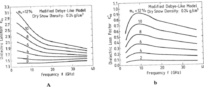
were measured for 62 snow samples at the frequencies between 3 GHz and 37 GHz by Hallikainen et aÏ. (1986) using a ftee-space transmission technique. The range of liquid water content (Lw) in the samples was between 1 and 12 percent. They applied an empirical modified Debye-like rnodeï to caïculate the permittivity and dielectric loss factors of wet snow. Figure 6 shows the effect of liquid water content on the dielectric behaviour of wet snow between 3 GHz and 37 GHz for a dry snow with an average density of P 0.24 g crn3.
t,fDpt
0 10 20 30 40
Frcuncy f ({iHz)
Figure 6: a- The spectral variation of the permittivity ofwet snow with snow wetness as a parameter; b - The spectral variation ofthe loss factor ofwet snow
with snow wetness as a parameter. The curves are based on the modifiedDebye-Ïike model (after Hallikainen et al.,
1986)
As shown in Figure 6b, the maximum value ofE,s was obtained at 9.0 GHz which agrees with the relaxation frequency of water at 0°C. Because of the large increase in the
Q Q
‘n
o L] L-.. CiL ‘u 11 1.0 0.9 0.8 .. 0.7 0.6 0.5 V, o -J C Q, G) cD A b 20 Frequency t t 0Hz)magnitude of dielectric loss factor for water (&‘) between 3 GHz and 6 GHz, there is a sharp increase in dielectric loss factor of wet snow (&‘) over this frequenoy raige. The attenuation constant of wet snow increases practically linearly with frequency up to 15 GHz. From 1$ GHz to 37 GHz, the average siope is slightlysrnaller.
3 INTERFEROMETRIC SAR
3.1 Tlieory
Since the first airborne radar interferometry application (Graham, 1974), interferometric SAR (InSAR) has been applied increasingly in the last decade for the measurement of Earth’s topography (technique description and review, Zebker et al., 1994a; Bamier and Hart, 1998,
surface changes - Askne and Hagberg, 1993; WegmtilÏer et ctl., 1995,
and surface feature movernents - Gabriel et aÏ., 1989; Goldstein et aÏ., 1993, Massonnet
et aÏ., 1995).
InSAR exploits the phase differences of two single-look complex SAR images acquired fi-om diffei-ent orbit positions sirnultaneously or at different times. The parent images contain information related to phase, coherence, backscatter amplitude, texture and amplitude differences. This information can be used to estirnate several geophysical quantities, such as topography, snow cover, vegetation, ground dispiacement (vertical and horizontal), hydrography, growth and dynamics of lake ice and soil characteristics.
The InSAR geometry in the plane of observation is shown inFigure 7. SAR data are acquired at the locations designated 1 and 2 and are processed to complex images S (x, y) A1 exp {çl
}
and S, (x, y) = A, exp{02}
where (x,y represents the azimuth and range imagecoordinates.
Subject to constraints on surface change and proximity of the orbits to one another, the two images may be registered and combined to produce an interferogram (Equation 4):
I(x,y) (4)
The phase of the interferogram is the phase difference between the two images. The unwrapped phase ((L)) may be related to the path difference (3)between two imaging locations. If the baseline, defined in ternis of orbit separation (B,) and tilt angle
(),
is known, then the measured difference in the interferogram phase (cÏ) between two points may be related to the change in range dR and the change in surface height dz(Ulander and Hagberg, 1993):2kB,,
[dz+cos9.dRJdØ+dØR, (5)
RsinO
where R is the range to the first point,
e
is the local incidence angle,k = 2rt/2is the radar wave number, 2L is the radar wave length.
And thus
B,, Bcos(&—) (6)
Where B,, is the perpendicular (normal) component ofthe baseline and
()
is the tilt angle.The tenn dRmay be systernatically removed from the interferogram to retain only the tenam dependent phase fluctuation d. In this case, each phase fringe (change in phase from Oto 2n) represents a relative change in elevation of
d
_%RsinO//23,,
t)
7For successful interferometry, the phase in the two images must be well correlated. The coherence, a measure ofthe phase correÏation, is defined as:
(s1
(x, y)5 (x,y)7=
Where
(s
(x, v)S (x, y) is the spatial average over aprocessing window.Lineof
sight h
n
(8)
y
Figure 7: Geometry ofrepeat-pass InSAR
The coherence lies in the range Oyl. If the coherence is large (close to unity), the phase in
two images is highly correlated between the two passes. If the coherence is srnall (close to zero), the phase is flot well conelated. Surface changes during the time between passes, such
as temporal changes in the geometric and electric properties of the surface, may reduce the
desired coherence. This contribution to the measured coherence, usually refeiied to as the scene coherence, can provide information on geophysical surface properties, however, other causes such as phase aberrations in the processor, differing imaging geornetries, and heterogeneous atmospheric conditions, may also lead to phase decorrelation.
3.1.1 Differeutial Interferometry
A development of the interferornetry scheme can be used to detect changes in topography. Suppose that two interferograms are fonned of a given target scene, taken at different times, and one subtracted from the other. If nothing has changed during the intervening period, there will be a constant phase difference everywhere. If, on the other hand, elevation changes have occurred, then these will show up as fringes in the differential interferogram.
This gives an extraordinarily sensitive means of measuring elevation changes. In fact, Differential Interferometry (DInSAR) is a measure of the small dispiacernents which have occurred in the scene between two image acquisitions (Gabriel et al., 1989). If there are changes during the image acquisition times, the interferometric phase will record any dispiacement of the ground along the radar une of sight that has occurred during the time interval between the two images.
The sensitivity of the phase to the topography increases with an increase in the baseline separating the two antenna locations at times of the data acquisitions. To generate a surface dispiacernent rnap it is necessary to remove the topographie signal from the interferogram. This can be achieved by either:
• simulating the topographie phase using a digital elevation model and with knowledge of the geometry of the interferometric system (two pass rnethod, e.g., Massonnet et al., 1993; Murakarni et aï., 1996);Or
• by generating two interferograms out of three or four SAR images of the same area, and computing the phase difference of the two or to eliminate the topographic phase signal common to both interferograms (three or four pass rnethod, Gabriel et aÏ., 1989; Peltzer and Rosen, 1995).
The sequence ofDInSAR images ofthe Landers earthquake (June 18, 1993) provided an ideal test for differential interferometry. Because the shallow depth of the epicentre, the earthquake produced spectacular surface rupture in an arid area less than three months afler the ERS-1 satellite began acquiring rada;- images in its 35-day orbital cycle (Massoirnet et aï., 1994a).
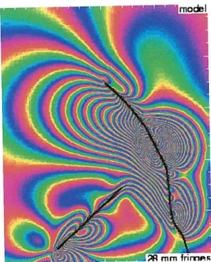
With 20 fringes in the shape of a crushed butterfly, the first earthquake interferogram
(Figure
8) illustrated the coseismic deformation field (Massonnet et al., 1993). The original study
launched many others (Peltzer et aï., 1994; Zebker et al., 1994b; Massonnet et al., 1994a; feigi et aï., 1995).
Each fringe denotes 2$ mm of change in range. The number of fringes increases from zero at the northern edge of the image, whcre no coseismic dispiacement is assumed, to at least 20, representing 560 mm in range difference, in the cores of the lobes adjacent to the fault. The asymmetry between the two sides of the fault is due to the curvature of the fault and the geometry of the radar. Black fines denote the surface rupture mapped in the field (Massonnet et aï., 1993).
Figure 8: Modeled interferogram with black unes denoting known fault unes and coloured fringes related to changes in surface elevat ion
3.1.2 Errors and limitations ofInSAR
The major limiting factors for topographic mappingand deformation monitoring using InSAR are:
• The limited measurement accuracy ofthe interferometricphase (phase noise; Barnier and Hart, 199$; Rodriguez and Martin, 1992);
• The variation in the wave propagation conditionsover the data acquisition period (atmospheric signal; Zebker and Rosen, 1997; Hanssen and Feijt, 1996; Goldstein,
1995; Mouginis-Mark, 1995);
• Repeat-pass temporal change ofthe backscatterproperty ofthe surface (temporal deconelation; Zebker and Villasenor 1992).
3.1.2.1 Phase noise
The phase differences which constitute the interferogram can be corrupted by phase noise, firstÏy due to the finite signal-to-noise ratio in each of the two images, and secondly due to the fact that, for a distributed target, the two signais corresponding to a given pixel are partially decorrelated (Zebker and Villasenor, 1992). This occurs because the contributions from the scatterers within the pixel add up with a slightÏy different phase reÏationship, since they are viewed from a slightly different angle. A larger baseline can resuit in a greater decorrelation effect. The phase noise can, of course, be reduced by averaging multiple looks, but at the expense of increasing the pixel size.
The effect of pixel deconelation on phase noise has been evaluated by Barnier and Hart (1998). Figure 9 shows the phase noise standard deviation as a function of coherence and number of looks. It is interesting to note that (for high coherence) averaging ofL independent complex interferogram samples reduces phase noise significantly.
3.1.2.2 Atmospheric perturbations
The determination of surface-changes using JiiSAR is based on the assumption that the radar signal propagation is unaffected by the atmosphere. This, however, is not the case. Path delays occur in both the ionosphere and the troposphere. Ionospheric path delay is caused by variations in the total electron content along the path and by moving ionospheric disturbarices. The former depends on the time of day and influences the whole scene
homogeneously. The latter may cause localized artefacts. The rnost severe atrnospheric effect, however, occurs in the troposphere. Its path delay consists of two components, the dominant dry part (about 2.3 ni in vertical direction) and the small but highly variable wet
part which is caused by the strong temporal and spatial variability of the water vapour concentration. It can take on magnitudes up to 30 cm. Artefacts in interferograms have been reported quite often and some of them have been assigned to atmospheric perturbations as in Massonnet et aï., (1994b), Massonnet and Feigi (1995) and Hanssen and Feijt (1996).
1 ai
80
60
4a
Figure 9: Standard deviation ofthe phase estimate as a function ofcoherence and number of independent samples L (after Bamier and Hart 1998)
These effects can cause misinterpretation in the order of centimetres of the defonnation fields at the surface derived from InSAR. For instance, a differential interferornetry chai-t of the KiÏauea volcano system, generated by data of the April and October mission ofSIR-C in 1994 was first interpreted as a demonstration of avolcanic lift of several centimetres. Later this tumed out to 5e just the atmospheric effects. These effects have been reported by Hanssen and Feijt (1996). Although recognized as one of the most important and challenging research topics for InSAR, only a few quantitative results have been published so far (e.g. Goldstein, 1995; Massonnet and Feigl, 1995; Tarayre and Massonnet, 1996). Especially in wet regions like the Netherlands, SAR images exhibit artefacts due to the temporal and spatial variations of atmospheric water vapour. Other tropospheric variations,
20
such as pressure and temperature, as well as ionospheric perturbations also induce distortions, but the effects are smaller in magnitude and more evenly distributed throughout the interferogram than is the wet tropospheric term.
3.1.2.3 Temporal decorrelation
The main lirniting factor for repeat-pass InSAR is the temporal change of the backscatter property of the surface between two satellite passes, the so-called temporat decorretation. Reasons for this may be due to volume scaflering in vegetated areas, especialÏy forest, changes in vegetation phenology, variations in sou moisture, lava flow, fieezing and thawing, and man-made changes. Temporal decorrelation is most prevalent for water surfaces and the lowest for desert or other arid areas with sparse vegetation. A loss of correlation, i.e. of scene coherence, makes the gathering of phase information more difficuit or even impossible. For instance, snow covered, agricultural and other vegetated areas suffer from severe temporal decorrelation. For snow decorrelation it couÏd be even a few hours depending on the change in temperature.
In many SAR images, decolTelation effects are visible even after just one day (ERS tandem mission), after a few weeks the complete scene can be almost deconelated. Qualitatively, it is lumwn that:
1) desert is better than dense forest;
2) dry conditions are better than wet;
3) long radar wave length is better than short;
4) urban areas and solid scatters such as houses, rocks, and corner reflectors hardly decorrelate;
5) water decorrelates within 0.1 s which means that repeat-pass InSAR cannot be applied over ocean surfaces;
6) agricultural activities lead to a loss of coherence for individual agricultural
fields.
3.2 The influence ofwet and dry suow on InSAR DEM’s 3.2.1 Dry condition
Interaction of radar with snow is a function of the snow properties. When snow is in a dry condition, its backscattering is minimal at C-band (Bemier and Fortin, 1991). Hence, the snow/ground interface is the main reflector. However, its higli refractive index creates a phase delay which varies linearly with the snow pack water equivalent (Granberg and Vachon,
1998). In this section the theory ofthese interactions will be elaborated.
Earlier elaborations ofthe distortion ofDEM’s by dry snow (Shi et al., 1997; Strozzi et aï, 1999; Guneriussen et aï., 2001) sec it as a resuit of refraction, analogous to that observed in the optical domain. AccordingÏy, assuming that the images are obtained when the gi-ound is covered with homogenous dry snow, the phase term in equation 5 is given by:
tota1 = øtopo+Ç5d
(9)
42z-=—AR+ç (10)
Where
2. is the radar wave length;
AI? the two-way difference in slant-range vector from sensor to the ground pixel, and ç5 is the two-way propagation difference in free air and snow.
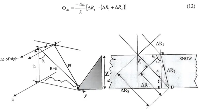
The radar beam vector will change because of the change in refraction due to difference in dielectric properties between air and snow (Figure 10).
Now ql, the dry snow phase term in equation 10 represents the difference in the two-way propagation with and without snow:
ds%ds
Line of sight
t1s
= _42T[/\R
—(,
+AR)] (12)Where
2: radar wave length; O: incidence angle; z: snow cover depth; n: snow refraction index.
y
X
Figure 10: Refraction change due to difference in dielectricproperties between air and snow
Using the geornetry illustrated in figure 10, we obtain:
—4r sin2 O. —n
= zcosU+
(5 I t? 2
—sin
e,
In dry snow conditions the complex pennittivity is governed by the dielectric properties of ice,
snow density, and ice particle shape (Haïlikainen and Winebrenner, 1992). This pennittivity is independent of the temperature because the permittivity of ice is & 3.17 in a range of ftequencies ftorn 10 MHz to 1000 GHz. Thus the permittivity of dry snow (e’d$) is only a function of density (p), which, under natural snow pack conditions usually varies over the range 0.2 to 0.5 g crn3 (Ulaby et aÏ., 1982).
Contrary to permittivity of dry snow (u), the imaginary part (ds) is much smaller. in
which case the value ofd can be found by puffing E’— O (Mitz1er, 1987).
Based on Mitzler (1987) the dielectric constant of dry snow is:
n2 E1+1.7p+0.7p2 (14)
Where (p,) is the snow density and
()
is dielectric constant (real part). For snow density in the0-0.6 g/crn3 range, a squar foot ofequation 14 given as:
n=Jr=1+0.85p (15)
Inserting equation 15 into equation 13, gives the reÏationship between interferornetric phase and changes in snow density and snow depth:
—4r sin2 û —(i +0.85p) z cos&.+ (16) z ,JZ.g5p)2_sjn2o
Since snow water equivalent given as:
$WEzrz.p (mm)
(17)
—4 SWE.p1(Sj112 —ï)— 0.85SWE $WE.p1.cos1 + t (18) J1+0.85p) —sin2O1
A simpïified forrn ofequation 18 is:
—4yr cos2&.+0.85p
ds = cosO1— .$WE
(19) cos2 O
+ï.7p+0.7 p2
This equation reveals that there exists a direct relation between the InSAR phase difference of dry snow and changes in snow water equivalent SWE. In other words, the interferornetric phase difference of dry snow is a function of the snow depth. Presence of the deeper dry snow
on the ground produces more delay of the phase during a round-trip.
The sensitivity of the algorithm was tested to sec how different parameters would control the phase difference obtained from radar round-trip (siant range) in the dry snow. Ibis is feasible because, the combination of the incidence angle (O) and snow density (p) may have different influence on the InSAR phase differences.
In a first sensitivity analysis we verified several combinations of these parameters, and indeed the incidence angle of sensors plays a very importantrole in phase differences of InSAR data due to hydrographical features of the medium. As we see in equation 19, this parameter has a crucial influence on InSAR phase.
Each sensor platform has a different incidence angle (O). To see how the actual and future operational radar satellites wouÏd react in regard ofthe developed algorithm (equation 19); we considered a wide range of incidence angle in the assessment. One of the most frequently used in interferometry SAR is the ERS Tandem Mission using ERS-1 and 2 was designed to provide the interferometric data with temporal delay of one day. The incidence angle of the two sensors was fixed at 23° upon which many theoretical studies in the InSAR domain are based. ENVISAT also has the sarne incidence angle.
Another satellite data source used frequently in interferometry SAR is the Canadian RADARSAT- 1. This SAR instrument can shape and steer its radar beam at C-band. A wide variety of beam widths are available to capture swaths of 45 to 500 km, with a range of 8 to
100 meters in pixel size and incidence angles of 20 to 49 degrees.
Using the rang of incidence angles available from these satellites we calculated the variation of hSAR phase differences in relation to incidence angles changes from 20 to 50 degrees. To facilitate the understanding of the SIIOW characteristics role on interferometric phase
difference, we also varied the dry snow densitywith three typical ones (0.3, 0.4 and 0.5 g cm3) as well as the snow depth from 5 cm to 100 cm withan interval of 5 cm.
In the second assessment of the sensitivity ofequation 19, we traced the variation of hiSAR phase differences versus the Snow Water Equivalent (SWE). We postulated a snow cover with
100 cm depth and with three density conditions (0.3, 0.4 and 0.5). AIl these variations in SWE
and density were also anaÏysed at various incidence angles. We particularly emphasized the 23° incidence angle of ERS I and 2.
3.2.2 Wet condition
When the snow changes to a wet condition (presence of liquid water), die irnaginary part shows very high sensitivity to the amount of liquidwater content (L; percent by volume). Cumming (1952) found that with increasing liquid watercontent of a dry snow from zero to
0.5 percent, the e” increased by more than one order of magnitude. This means that the
depth penetration of microwaves decreases significantly and the scattering cornes primariÏy from the air-snow interface. Thus, in ideal conditions, the depth of wet snow may be rneasured simply by subtracting the DEM produced for snow-free terrain from that generated for terrain covered by wet snow.
The roughness of the wet snow surface lias a strong influence on the backscatter, consequently in interferometric processing, wet snow cover is considered as a distortion superimposed on the topography. Therefore the “snow phase” in figure 10, (y) is a reduction in the two-way path given as:
4yr
G÷ ——-—(ARG —AR)
(20)
‘t
Where:
G+Ws is the phase difference related to the altitude ofthe
ground covered by wet snow;
ARG is two-way path of snow ftee ground;
And is two-waypath ofwet snow cover.
Thus, in summary, the DEM produced when the snow cover is wet represents the ground surface elevation, to which the depth of snow bas been added. Thus, differential InSAR can measure both snow depth and density, the former on occasions when the snow surface is wet,
and the latter when the snow cover is dry.
3.3 Theoi-etical analysis
In this section we analyse the theoretical researcli phase where we explored the relationship of interferornetry SAR phase difference with Snow Water Equivalent. The phase difference sensitlvity of developed algorithm (equation 19) was verified in comparison with the variation of existing parameters.
In the first stage the crucial influence ofvariation of incidence angle of the sensor on radar siant range was recogiised.
The curves in Figure 11 show the variation of interferornetric phase difference for sensor incidence angle (from 20 to 50 degrees). The coloured curves represent the snow cover depth from 5 to 100 cm having the density of 0.3 g cm3.