To cite this version :
Courbaud, Benoît and Pupin, Cyrille and Letort, Anthony and Cabanettes, Alain and Larrieu, Laurent Modelling the probability of microhabitat formation on trees using cross-sectional data. (2017) Methods in Ecology and Evolution, vol. 8 (n° 10). pp. 1347-1359. ISSN 2041-210X
O
pen
A
rchive
T
OULOUSE
A
rchive
O
uverte (
OATAO
)
OATAO is an open access repository that collects the work of some Toulouse researchers and makes it freely available over the web where possible.This is an author’s version published in : http://oatao.univ-toulouse.fr/19608
Official URL : https://doi.org/10.1111/2041-210X.12773
Any correspondence concerning this service should be sent to the repository administrator :
Running title: Formation of microhabitats on trees
Modelling the probability of microhabitat formation on trees using cross-sectional data
List of authors: B. Courbaud a, C. Pupin a, A. Letort a, A. Cabanettes b, L. Larrieu b,c, a
Université Grenoble Alpes, Irstea, UR EMGR, 2 rue de la Papeterie-BP76, F-38402 St-Martin-d’Hères, France,
b
INRA, UMR 1201 DYNAFOR, Chemin de Borde Rouge, Auzeville, CS 52627, 31326 Castanet Tolosan cedex, France
c
CRPFMP, 7 chemin de la Lacade, 31320 Auzeville Tolosane, France
Corresponding author: Benoit COURBAUD, Université Grenoble Alpes, Irstea, UR EMGR, 2 rue de la Papeterie-BP76, F-38402 St-Martin-d’Hères, France. [email protected] Tel: (33) 4 76 76 27 62 Fax: (33) 4 76 51 38 03
Emails: [email protected]; [email protected]; [email protected]; [email protected]; [email protected];
Summary
1. Context: Tree-related microhabitats (TreMs), such as trunk cavities, peeled bark, cracks or sporophores of lignicolous fungi, are essential to support forest biodiversity because they are used as substrate, foraging, roosting or breeding places by bryophytes, fungi, invertebrates and vertebrates. Biodiversity conservation requires the continuous presence of TreMs in a forest. However, little is known about their dynamics. Moreover, we usually have only cross-sectional TreM data (observations of many trees at a single time), making it difficult to estimate TreM formation rates.
2. Method: This study adapted the methods of survival and reliability analysis to model the rate of TreM formation per unit of diameter increment as a function of tree diameter at breast height (DBH). We tested three variants of this model: the TreM formation rate independent of, proportional to or increasing non-linearly with DBH. We calculated the likelihood of the models, considering cross-sectional observations either of TreM presence/absence or TreM number on trees of different sizes. We calibrated the models in six sub-natural montane forests dominated by European beech (Fagus sylvatica) and silver fir (Abies alba) – in the French Pyrenees. Assuming an annual DBH increment value, the annual formation rate of TreMs was predicted both at the level of the tree and at the level of the forest stand.
3. Results: This method provided a coherent framework to model the probability that a TreM forms on a tree during a unit growth step and produces realistic predictions of TreM
accumulation on trees. TreM formation accelerated as trees grew for A. alba but not for F.
sylvatica. The TreM formation rate was twice as fast on F. sylvatica as on A. alba. We
estimated a formation of 0.82–1.28 TreMs/ha per year and 0.5–0.9 TreM bearing trees/ha per year in the sub-natural forests studied.
4. Synthesis and applications: This method makes rigorous modelling of the formation of TreMs possible during the growth of trees and forest stands. The quantitative evaluation of
TreM fluxes will help to design forest biodiversity conservation strategies favouring the development and temporal continuity of TreMs.
Tweetable Abstract
The rate of TreM formation per unit diameter growth was modelled as a function of tree diameter at breast height (DBH), and the model was calibrated considering cross-sectional observations TreMs on trees of different sizes. The model predicted realistic TreM formation rates at the tree and stand levels in forests dominated by Abies alba and Fagus sylvatica. This approach opens new perspectives to the analysis of forest biodiversity conservation strategies.
Key words: Tree-related microhabitats, biodiversity, survival analysis, reliability analysis, tree cavity, tree hollow, Abies alba, Fagus sylvatica, Bayesian statistics, habitat conservation, time-to-event
1. Introduction
Forest ecosystems cover approximately 30% of the world’s land surface (Pan et al., 2013)
and play a key role in terrestrial taxonomic biodiversity (Lindenmayer and Franklin, 2002). However, forest reserves account for only about 11% of the global forest area (Bollmann and Braunisch, 2013). Consequently, the conservation of forest biodiversity also depends on forests without a specific protection regime. The role of deadwood as a habitat for many insects, fungi or lichen species has been recognized for decades (Lachat et al., 2013; Müller and Bütler, 2010; Seibold et al., 2015; Gossner et al., 2013; Speight, 1989; Stokland et al., 2012; Bobiec et al., 2005). More recently, research has focused on tree-related microhabitats (TreMs), which are singular morphological features developing on the trunks or branches of trees, such as cavities, cracks, peeled bark, root buttress concavities, epiphytes or sporophores
of saproxylic fungi. TreMs are used as substrate, foraging, roosting or breeding places by many species of taxa as diverse as lichens, bryophytes and fungi, micro-crustaceans, insects (e.g. Coleopterae, Dipterae, Hymenopterae), spiders, amphibia (e.g. Anoura, Urodela), birds (e.g. Picidae, Strigidae) and small mammals (e.g. Chiroptera, Gliridae, Mustelidae) (Stokland
et al., 2012; Winter and Möller, 2008). Some taxa are highly dependent on TreMs: more than
40% of birds in French forests use tree cavities or cracks for breeding (Blondel, 2005), and in Europe, roughly half of the insect species that breed in dendrothelms (i.e. water-filled holes) are strictly dependent on this habitat (Dajoz, 2007). TreMs are considered as relevant surrogates of direct biodiversity measures (Winter and Möller, 2008), particularly for saproxylic beetles (Bouget et al., 2014; Bouget et al., 2013), and are already integrated into some practical biodiversity assessment tools used by forest managers (Larrieu and Gonin, 2008). In addition, conservation of biodiversity in managed forests can be improved by protecting high-biodiversity-value trees such as trees bearing TreMs and dead trees from harvesting. This strategy, called the retention approach in forestry, appeared in the 1980s in the USA (Franklin et al., 1981; Thomas et al., 1979) and has aroused increasing interest in other parts of the word since then (Bütler et al., 2013; Larrieu et al., 2012; Lindenmayer et al. 2012; (Fedrowitz et al., 2014). The idea first emerged as an alternative to clearcutting and is probably not sufficient to balance the impact of intensive logging on biodiversity. However, it is increasingly applied in selective harvest operations, where it is proposed as a means to integrate conservation into forest management (Gustafsson et al., 2013). The retention of several high-biodiversity-value trees per hectare is therefore mandatory to obtain sustainable forest management certificates (FSC, 2016; PEFC, 2010).
TreMs are structures that form on trees during their development and disappear when the trees are harvested or die and decompose. It is therefore essential to quantify the TreM formation rate and compare it to tree mortality and tree harvesting rates in order to explain variations of TreM density in a forest stand. Several authors have shown that most TreM types are more frequent on snags, large living trees and broadleaved species (Larrieu and Cabanettes, 2012; Larrieu et al., 2014a; Vuidot et al., 2011). However, these results do not give direct indications on the rate of TreM formation on trees. Using a different approach, (Lindenmayer et al., 1993) characterized the types and numbers of TreMs expected on trees of different life forms and diameters at breast height (DBH). On this basis, Ball et al. (1999) and Gibbons et al. (2010) developed a transition matrix model making it possible to simulate changes in forest structure, and therefore changes of TreM distribution. However, this
approach relies entirely on the estimation of transition probabilities between life forms, a point little described by the authors. A simple way to estimate a TreM formation rate would be to use the variations of TreM number on trees observed repeatedly. Unfortunately, such repeated TreM measurements are still largely missing because of the relatively recent interest researchers have taken in this subject (Lindenmayer et al., 2011). Moreover, trees have rarely been labelled in the field in previous studies, making new measures on the same trees
impossible. TreM types such as woodpecker holes are rare and the detection of their
formation requires large tree samples (Larrieu et al., 2014a). Huge measurement efforts will be necessary before large databases with repeated observations of TreMs are available.
Inferring the rate of TreM formation from cross-sectional data (observation of several individuals representing different development stages) is required because of data
availability. However, this poses several challenges. First, we usually do not know the age of trees. It is therefore difficult to relate TreM formation to a time scale. Second, observations
are censored: we do not know exactly at what time the TreM formation event has occurred or will occur. If we observe a TreM on a tree, we only know that the formation of the TreM occurred before the time of observation (this is called left censoring). New TreMs will perhaps form on the tree in the future, but we do not know when (this is called right
censoring). Survival analysis and reliability analysis are other fields of research challenged by modelling the occurrence of events during the development of a population. These techniques analyse the expected duration of time until one or more events occur, such as death in biological organisms and failure in mechanical systems, and the rate of these events (Hosmer et al., 2008; Meeker and Escobar, 1998). They answer questions such as: what is the proportion of a population which will survive past a certain time? Of those that survive, at what rate will they die or fail? How do particular circumstances or characteristics increase or decrease the probability of survival?
The objective of this study was to test whether we could transpose the concepts of survival and reliability analysis to model the event of TreM formation on trees and apply it to cross-sectional data. We considered that the test would be successful if this approach provided a logical and coherent framework for the analysis of the data as well as good predictions. We also tested three biological hypotheses. The first hypothesis postulates that TreM formation accelerates during tree growth, in relation to the observation of a disproportionate proportion of TreM bearing trees among large trees (Larrieu and Cabanettes, 2012). The second one advances that the rate of TreM formation is higher on broadleaved than conifer trees of similar size, in agreement with the observation of a higher frequency of TreM-bearing trees on broadleaf trees (Larrieu and Cabanettes, 2012). The third one hypothesizes that at the stand level, the rate of TreM formation is not strongly correlated to TreM density, meaning that the dynamic and the static perspectives are complementary. We applied the survival
analysis approach to TreM cross-sectional observations coming from mixed sub-natural forests in the Pyrenees dominated by a broadleaved species, European beech (Fagus
sylvatica) and a coniferous species, silver fir (Abies alba). These two tree species are
important late successional species in Europe and have a great economic and ecological importance. Moreover, tree architecture, microhabitat density, wood decay rate and biocenosis differ substantially between broadleaves and conifers (Larrieu et al., 2014b).
2. Material and methods 2.1. Data
The data (Larrieu, 2017) were recorded in six forests unmanaged for more than 100 years located in the central Pyrenees mountain range (Lat: 42°45′N-43°3′N – Long: 0°9′W-0°36′E), at the montane altitude level ( – m). Observations were made in the summers of
2008 and 2009 (Larrieu et al., 2012) on 37 circular plots with random locations within areas defined by their accessibility. We used the constant angle method (Bitterlich, 1984) in order to increase the proportion of large trees in the sample and obtain a better balance between observations of small and large trees and a better balance between observations of trees with and without TreMs in the data set. Trees above 2.5 cm DBH were observed when the ratio between their DBH and the distance to the center of a plot was more than 1/50. The radius Ri of the sampled area therefore increased as tree size increased ( ). For stand level
applications, we weighted each tree depending on the area sampled for its DBH. For each tree, the DBH outside the bark, the species of the tree and all the TreMs on the trunk beneath and within the tree crown were recorded, in reference to a list of seven TreM types: (i) cavities whose entrance was wider than 3 cm, (ii) missing bark area covering at least 100 cm2, (iii) cracks in the trunk 1–5 cm wide, (iv) dendrothelms greater than 3 cm wide at the entrance, (v) sporophores of saproxylic fungi (polypores and pulpy agarics), (vi) epiphytes
(Yvi and foliose lichens) and (vii) dead-wood in the crown. Every tree was observed on all sides, from its foot and from a distance of dozens of meters using binoculars, to make as exhaustive an observation as possible. The data set was composed of A. alba trees,
F. sylvatica trees and 110 trees of other broadleaved species, each of which was represented
by fewer than 35 individuals (Buxus sempervirens, Betula pubescens, Sorbus aucuparia, Tilia
platyphyllos, etc.). Five hundred trees had at least one TreM and 749 trees had no TreMs.
Since several TreM types were recorded less than ten times per species, we considered that the data set was too small for a detailed analysis and we grouped all the TreMs in a single type and all species other that A. alba and F. sylvatica in a single group. We also used DBH increment records of the French National Forest Inventory in the “High Pyrenees” ecological region between 900 m and 1750 m elevation (sample of 757 A. alba trees and 2105 F.
sylvatica trees), reaching a rough estimate of the annual DBH increments of the trees in the
data set of 2.34 mm/year for F. sylvatica (SD=1.7 cm), 3.74 mm/year for A. alba (SD = 2.73 cm) and between 1.11 mm/year (Crataegus monogyna) and 4.96 mm/year (Acer platanoides) for the other species
2.2. Adaptation of the survival analysis approach to the formation of the first TreM Scientists practicing survival or reliability analysis process the time to an event as a random variable (Hosmer et al., 2008; Meeker and Escobar, 1998; Clark, 2007). This event is usually the death of an individual or the failure of a machine. We considered the event of interest as the formation of a TreM. Survival and reliability analyses are usually performed on repeated measures describing the development of a cohort of individuals observed several times. Having only cross-sectional observations of trees of different DBHs, we replaced time with DBH in the analysis. However, this implies the assumption that TreM bearing trees had a similar rate of mortality than other trees during their growth (see 4.4.).
Let us define D as a random variable corresponding to the DBH of a tree when it contracts its first TreM. Following the survival analysis theory, we can define five related functions: is the probability that no TreM forms on a tree before it grows to diameter d This is
analogous to a survival function (probability of still being alive when reaching age t). (eq. 1)
is the probability that the first TreM forms on a tree before it grows to diameter d.
is the cumulative distribution function (CDF) of the random variable D. F(d) can also be interpreted as the probability that a tree observed at diameter d carries at least one TreM. This interpretation means that it is possible to estimate F(d) with our data.
(eq. 2)
is the probability density function of the random variable D or event density. The
function f(d) describes the distribution of DBHs at which the first TreM appears on the trees of a population. If F is differentiable,
(eq.3)
is the hazard rate, defined as the rate of formation of the first TreM at diameter d, on
condition that the tree has contracted no TreM before (that is, D ≥ d). The hazard function h(d) deserves special attention because it directly describes the process of TreM formation and how this process changes during diameter growth.
H(d) is the cumulative hazard function, describing the "accumulation" of the hazard over
growth.
(eq. 5)
These five functions are closely related but provide complementary descriptions of the relation between TreM formation and tree DBH. We will see below that F(d) is especially useful to estimate the parameters of the model, whereas h(d) provides the more direct description of the TreM formation process and H(d) is used in discrete time simulations.
2.3. The Weibull family of functions used to model a monotonic change of hazard with DBH
Survival analysis theory has identified efficient parametric functions that lead to interpretable forms of the hazard function h(d). The most classical form for f(d) is the Weibull function with two parameters: a shape parameter k and a scale parameter . If f(d) is a Weibull distribution, the hazard function is simply a power function of DBH. The functions are written as follows: S( (eq. 7) (eq. 8) (eq.9) (eq.10) (eq.11)
If k = 1, the hazard is constant and does not depend on DBH. This might suggest random external events are causing TreM formation. In that case, f(d) reduces to an exponential distribution.
If 0 <k < 1, the hazard declines as DBH decreases.
If k>1, the hazard rises as DBH increases. This means that trees without any TreM become increasingly susceptible to contracting their first TreM during an infinitesimal growth step as their DBH increases. The corresponding process is called “ageing” in survival theory and
corresponds to a maturation process in this example. If k=2, hazard increases proportionally with increasing DBH. In that case, f(d) reduces to a Rayleigh distribution.
Summary statistics can be calculated for D. If f(d) is a Weibull, E(D) and Var(D) are related to a gamma function. The median of the expected D at which the first TreM forms is expressed simply as:
(eq.12)
2.4. Formation of successive TreMs
If we assume as a first approximation that the formation of TreMs during an interval of time is influenced by neither the presence/absence of a previous TreM nor the number of previous TreMs on the same individual, the formation of successive TreMs is a Poisson stochastic point process (Meeker and Escobar, 1998; Rausand and Hoyland, 2004). The probability of formation of n TreMs during tree growth to DBH d is:
(eq. 13)
is the expected number of TreMs at DBH d: (eq. 14)
is the recurrence rate of TreM formation, assuming that is differentiable,
(eq.15)
In a Poisson point process, the recurrence rate is equal to the hazard rate h(d) of
formation of the first TreM, and the expected number of TreMs is equal to the cumulative hazard H(d) (Rausand and Hoyland, 2004).
2.5. Model calibration
We tested two approaches for model calibration. We considered first the binary variable corresponding to the presence (yi=1) or absence (yi=0) of at least one TreM on tree i. The likelihood function of a set of parameter values given the observation of TreM
presence/absence on a single tree of DBH is equal to a Bernoulli probability distribution with a success probability of . If we assume that TreMs form independently on different trees, the likelihood of a set of parameter values given the observations of
TreM presence/absence on N trees is: (eq.16)
We then considered the count variable corresponding to the number of TreMs ni observed on tree i. The likelihood function of a set of parameter values given the observation of ni TreMs on a single tree of DBH is equal to a Poisson probability distribution with a mean of . If we assume that TreMs form independently on different trees, the likelihood of a set of parameter values given the observations of the distribution of
trees having various numbers of TreMs in a set of N trees is: (eq.17)
We tested three hypotheses concerning the shape of the hazard rate function and the probability density function f(d) (i) Hypothesis 1: k=1, is independent of d and f(d) is an Exponential distribution function. (ii) Hypothesis 2: k=2, is proportional to d and f(d) is
a Rayleigh distribution function. (iii) Hypothesis 3: k is a positive exponent to estimate,
is a power function of d and f(d) is a Weibull distribution function.
We fitted the three models on our data set with a Bayesian approach using the “runjags” package (Denwood, 2016) in the R software (R Development Core Team, 2005). The code is provided in Appendix 1. We combined all the trees of the six forest sites without modelling any site effect. For the three models, we chose the parameter to be a gamma prior
distribution with a mean of 100 and a variance of 500: . For
the Weibull model, we chose the parameter k to be a gamma prior distribution with a mean of 2 and a variance of 4: . For each model, Monte Carlo Markov (MCMC) sampling chains of values were used with the first values as
the warm-up stage. We checked MCMC convergence using the criteria (Gelman et al.
2013).
2.6. Discrete-time simulation of TreM accumulation on trees and model evaluation The application of the model depends on its use in simulations. In forest dynamics,
simulations are usually made using a discrete time approach with annual time steps. If time steps are sufficiently short, we can assume that no more than one TreM can form during a time step. In this case the probability that a TreM forms on a tree during a time step (t, t+1) is:
If f(d) is a Weibull,
(eq. 19)
The model’s capacity to represent the process of TreM formation on trees correctly was assessed by simulating the past growth of the trees in the data set from an initial DBH of 7.5 cm up to their current DBH and the accumulation of TreMs during this growth. For one prediction, we drew a vector (k, ) in the MCM chains. For successive annual time steps, we calculated the initial and final DBH of the trees assuming constant increments equal to the National Forest Inventory mean DBH increment for the species in the study area. For each tree and each time step, the probability of formation of a TreM was calculated using
equation (19), and a Bernoulli trial was conducted to determine whether or not to add a new TreM to the tree. At the end of the simulation, we calculated the predicted proportion of trees carrying at least one TreM per DBH class of 10 cm, and the predicted proportion of trees carrying zero to six TreMs in the population. We replicated the simulations 1,000 times and obtained a distribution of 1000 predicted values of proportions of trees carrying at least one or zero to six TreMs. We then calculated % intervals of these predicted values, to compare
predictions and observations.
For each type of prediction, we calculated a set of three predictive loss criteria proposed by (Gelfand and Ghosh, 1998). This approach is based on the calculation of a goodness-of-fit measurement characterizing the distance between the predicted values and the observed
value, and a penalty term characterizing the variance of the predictions. The best model is
the model with the lowest values for these criteria. This approach makes it possible to compare both nested and non-nested pairs of models and responds to model over- or
under-fitting without requiring the arbitrary choice of a penalty depending on the number of parameters.
(eq. 20)
(eq. 21)
(eq. 22)
is the observation for tree i in the data set, is the mean of the predictions for tree i over simulation replications and is the variance of these predictions.
2.7. Application: predicting the rate of TreM formation at the forest stand level
To analyse the rate of formation of TreMs at the stand level, new simulations were carried out using the observed DBH of each tree in the data set as an initial state. For this section, only the Rayleigh model was used because of its good predictive performance and simplicity
(see § 3.2.). We sampled 1000 estimates of parameter in the MCM chain and made 1000 predictions of TreM formation during an annual diameter increment for each tree. Taking into account the sampling area corresponding to the DBH of each tree (constant angle sampling method, see § 2.1.), we calculated a predicted distribution of TreM formation rates per year and per hectare for each of the six forests. We then used linear regression to analyse the relation between the forest’s TreM formation rate and the forest’s TreM density or TreM bearing tree density.
3. Results
3.1. Relationship between TreM formation rate and tree diameter
Model calibration using the observation of the presence/absence of TreMs (likelihood function (16)) or the observation of the number of TreMs on trees (likelihood function (17)) gave very close results. We present the detailed results of the first method for the two dominant species (F. sylvatica and A. alba) in the main text and figures and provide the results of the second method in Appendix 2.
criteria values (Gelman et al. 2013) were less than , revealing a good convergence of the
MCMC chains for the three models: Exponential, Rayleigh and Weibull. Uncertainties were reasonably small, as shown by the credible intervals of the parameters (Table 1) and the confidence envelopes of the functions h(d), F(d) and f(d) (Figure 1). Higher values of λ for A.
alba than F. sylvatica (Table 1) translated into lower TreM formation rates for A. alba than F. sylvatica at all diameters and for all models (Figure 1). The TreM formation rate for A. alba
was for example only one-third of that for F. sylvatica in the Rayleigh model. The median expected diameter D at which a tree contracts its first TreM was therefore higher for A. alba than F. sylvatica: 88 cm [79–98] for A. alba (median and 95% confidence interval of the 1000 medians of D calculated over 1000 simulations) and 35 cm [30–42] for F. sylvatica with the Exponential model, 74 cm [70–78] for A. alba and 45 cm [41–49] for F. sylvatica with the Rayleigh model, 73 cm [66–82] for A. alba and 42 cm [34–50] for F. sylvatica with the Weibull model. These figures also show that the expected DBH of the first TreM formation estimated by the Rayleigh and Weibull models were quite similar and contrasted with the values estimated by the Exponential model. Uncertainties were higher for the group of diverse species, probably because of differences in growth and TreM formation rates among this group’s species. However, the parameter estimates were reasonable and rather close to the values for F. sylvatica.
The shape of the hazard function , which describes how the TreM formation rate
changes with tree DBH d, differed strongly among models (Figure 1). By construction, h(d) did not depend on d in the Exponential model. In contrast, h(d) increased linearly as d
increased in the Rayleigh model and showed a divergence between F. sylvatica and A. alba at higher. The Weibull model was more flexible because of the combination of two parameters k and λ. The hazard rate h(d) of the Weibull model increased almost linearly with d for A.
alba. However, for F. sylvatica, the hazard rate increased non-linearly as d increased because
of a mean estimate of 1.6 for parameter k, i.e. an exponent of k – 1 = 0.6 in the relation h(d). Because of this non-linearity in the Weibull model, the differences in hazard rate between the two species were maximum at medium values of d and then diminished for larger trees (Figure 1).
3.2. Models’ capacity to simulate the process of TreM formation
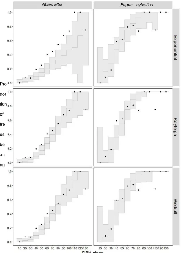
For A. alba, the predictive loss criteria of the proportion of TreM bearing trees per DBH class indicated a lower performance of the Exponential model compared to the Rayleigh and Weibull models (Table 2). For F. sylvatica, the three models showed a comparable performance. A graphical analysis (Figure 2) showed that this poor performance of the Exponential model for A. alba came from a prounced underestimation of the proportion of TreM bearing trees at huge DBHs, revealed by a discrepancy between the predictive envelopes and the data points. The correspondence between the predictive envelopes of the Rayleigh or Weibull models was more satisfying despite several data points slightly outside of the envelopes. For F. sylvatica the observations themselves did not show a clear pattern, especially in classes of large DBHs represented by a few individuals. The three models nevertheless managed to predict medians that increased monotonously as DBH increased and predictive envelopes covering most data points.
For both species, the predictive loss criteria of the proportion of trees in classes of zero to six TreMs did not distinguish the performance of the three models (Table 2). The graphical analysis (Figure 3) showed, however, that the three models slightly overestimated the
proportion of A. alba without any TreM and slightly underestimated the proportion of A. alba with a single TreM. For F. sylvatica, the three models underestimated the proportion of trees with one or two TreMs and slightly overestimated the proportion of trees with three TreMs or more.
Together, the tests identified the Rayleigh model as a good compromise between
performance and simplicity for A. alba. The two models simulating an increase of the rate of TreM formation with DBH over-performed the model simulating a constant rate of TreM formation for this species. For F. sylvatica, the three models gave comparable results. The best compromise between performance and simplicity could therefore be the Exponential model, simulating a constant TreM formation rate during tree growth.
3.4. TreM formation at the stand level
The individual probability of annual TreM formation was 0.52% chances per year [0.15%– 0.98%] (median and 95% predictive interval) for A. alba trees and 0.95% chances per year [0.31%–1.69%] for F. sylvatica trees in the forests studied. The mean predicted rates of TreM formation at the stand level varied from 0.82 to 1.28 TreM per ha and year depending on the forest (Table 3). This number could be multiplied by up to five in some simulations because of the uncertainty about the estimate of parameter lambda and of the stochasticity of the Bernouilli trials. These mean predicted rates of TreM formation corresponded to 0.47–0.69 TreMs per year for 100 trees larger than 17.5 cm, 1.48–2.43 TreMs per year for 100 TreM
bearing trees or 1.04–1.99 TreMs per year for 100 TreMs already present. The time required to reconstitute the TreMs present in the stands can be estimated as the inverse of the latter rate: between 100/1.99 = 50 years and 100/1.04 = 96 years. The predicted rates of new TreM bearing tree formation (i.e. trees receiving their first TreM) varied from 0.5 to 0.9 new TreM bearing trees/ha per year.
The regressions between the TreM formation rate at the stand level and the density of TreMs or the density of TreM bearing trees showed that only these two co-variables were not
capable of explaining the differences of TreM formation rates among forests (non-significant effects at a level of 5%).
4. Discussion
4.1. Survival analysis provides a change of perspective for TreM studies
Our adaptation of the survival and reliability theory appeared to be an efficient framework for the modelling of TreM formation. This approach made it possible to calibrate the relationship between the TreM formation rate and the DBH of a tree using cross-sectional data. Discrete time simulations of tree growth and TreM formation produced good predictions of the resulting distribution of TreMs in our forests.
This approach brings a key change of perspective in the study of TreMs. Most previous studies have concentrated on analysing the distribution of TreMs in a forest from a static perspective. Generalized linear models based on Poisson distributions have been used to analyse the number of TreMs of a given type on trees (Lindenmayer et al., 1993) or the number of TreM types per tree (Vuidot et al., 2011; Larrieu et al., 2014a). Logistic models have also been used to analyse the presence/absence of different TreM types on trees (Larrieu
et al., 2014a; Vuidot et al., 2011). These studies did not connect the distributions of TreMs
have done so by considering their models as the cumulative distribution function of a TreM
formation process. In contrast, our approach focuses on the estimation of the TreM formation
rate and the simulation of TreM accumulation during tree growth. Herein, we concentrated on Weibull family models because they represent the hazard rate with a simple power function of DBH, making it easy to test the three basic hypotheses: that the hazard is independent, continuously decreasing or continuously increasing with DBH. Other distributions defined in
have been proposed as probability density functions in survival and reliability analyses, such as the Gompertz, the gamma, the logistic, the generalized gamma, the log-normal, the log-logistic, etc. (Meeker and Escobar, 1998). They lead to more complicated and less flexible hazard functions. Moreover, they often lead to predictions very close to those made with a Weibull model. It is recommended to use these more complex functions only when they are justified by prior knowledge of the shape of the hazard function (Hosmer et al., 2008). We therefore started with the most simple hazard function in this methodological paper.
4.2. The relationship between TreM formation and tree growth depends on tree species. Several earlier studies showed that the presence and number of TreMs on a tree are related to its diameter and species (Larrieu and Cabanettes, 2012; Vuidot et al., 2011; Winter et al., 2015). Moreover, Larrieu and coauthors (Larrieu and Cabanettes, 2012; Larrieu et al., 2012) observed a disproportionate abundance of TreMs on very large trees. The better performance of the Rayleigh and the Weibull models over the exponential model for A. alba supports the idea that the TreM formation rate increases as DBH increases, i.e. that TreM formation accelerates during tree growth. This seems sound from an ecological point of view given that events such as breakings of large branches or cavities made by nesting birds should occur with a higher probability on large trees. However, for F. sylvatica, the three models gave
comparable results. The acceleration of TreM formation during tree growth is therefore not clear for this species. This acceleration could also be an artefact if TreMs influence tree mortality in such a way that small trees with TreMs die faster than large trees with TreMs. We obtained clearly higher estimates of TreM formation rates for F. sylvatica than for A.
alba. This result is in agreement with previous authors (Larrieu et al., 2012; Vuidot et al.,
2011), who observed that there were more TreMs on F. sylvatica trees than on fir trees of the same diameter. They also showed that cavities, missing bark and dendrothelms were mainly associated with F. sylvatica, whereas more diverse TreM types were found on A. alba. This difference in TreM types could explain the differences in the shape of the relationship between hazard rate and DBH that we found between these two species. Studies on more species are needed to explore the generality of these results. We expect that a difference between broadleaved and coniferous species will remain rather consistent because they have different crown architectures and different bark and wood properties: broadleaves have more large branches prone to breakage and more branch forks, usually have a thinner bark and their wood decomposes much faster, all phenomena facilitating faster development of TreMs such as cavities. Moreover, in this study, the parameter values obtained for the group of diverse broadleaved species was much more similar to values obtained for F. sylvatica than for A.
alba.
4.3. TreM dynamics as an indicator of potential biodiversity change
Our prediction of a formation of 0.82–1.28 TreMs per ha and year gives an order of magnitude for temperate montane mixed forest stands with a high degree of maturity. However, this figure represents only TreMs formed on living trees and should be complemented by TreMs formed on standing dead trees (Larrieu and Cabanettes, 2012). TreM formation in managed stands should be lower because of a reduction of large trees,
dead trees, and a tendency of forest managers to eliminate trees with TreMs negatively impacting wood quality (Larrieu et al., 2012). However, TreMs such as missing bark areas and dendrothelms can also increase because of harvesting (Larrieu et al., 2014a; Larrieu et
al., 2012) if trees are damaged by the falling and logging of their neighbours.
The average formation of 1.04–1.99 new TreMs/year for 100 TreMs corresponds to 50–96 years required to reconstitute the TreMs of our stands. This result strengthens the idea that approximately 100 years without logging are necessary for a montane forest stand to acquire a structure comparable to a natural stand (Larrieu et al., 2012). This roughly corresponds to one-third of the time necessary for a forest stand to complement a full sylvigenetic cycle (Larrieu et al., 2014b).
Estimating a flux of TreMs completely requires balancing TreM formation with tree mortality and decomposition. The annual mortality rate of very large trees in temperate forests is usually less than 0.5% (Vieilledent et al., 2010; Vieilledent et al., 2009; Monserud and Sterba, 1999). This would correspond to a mortality of 0.24–0.4 TreM bearing trees/ha per year in our forests, compared to our prediction of 0.46–0.89 new TreM bearing trees/ha per year. Several types of TreMs can be considered as indicators of tree senescence (for example fungi sporophores) and it is probable that the mortality of trees carrying these TreMs is higher than the average. However, Larrieu et al. (2014b) showed that the availability of
TreMs appears to be rather stable in unmanaged mountain mixed forests of different development stages, in terms of both quantity and diversity.
Neither the density of TreMs nor the density of TreM bearing trees was sufficient to predict the differences in the annual TreM formation rate between the sub-natural forests studied herein. This means that the presence of TreMs or TreM bearing trees does not guarantee a high TreM formation rate. This point is even more crucial in managed forests since forest management can shut down the formation of new TreM bearing trees despite the retention of
some old and large TreM bearing trees if the harvesting diameters are too low in the rest of the population. The tree retention approach alone therefore appears insufficient to maintain forest biodiversity over the long term. Senescence islands where a natural forest cycle can occur must also be preserved, and within managed areas a conservation strategy based on the functioning and the dynamics of the ecosystem is necessary. Indirect evaluations of forests’ potential biodiversity are usually based on state variables such as TreM density or dead-wood volume observed at a given time (Larrieu and Gonin, 2008). Taking into account flux
variables such as the TreM formation rate would empower these evaluations by providing an indication of the potential changes in biodiversity we can expect in the future.
4.4. Limits and perspectives
This study focused on the general applicability of survival analysis to the modelling of TreM formation. The good prediction capacity of the model used justifies the refinement of this approach and its extension to more complex situations. Certain assumptions were nonetheless simplified and must be kept in mind.
We treated cross-sectional observations of TreMs on trees of different DBHs as if they were longitudinal observations describing the accumulation of TreMs on a cohort of growing trees. This approach requires first that TreMs do not disappear on the trees, and second that the presence of TreMs does not modify the tree mortality rate. Some exceptions can be found to the first assumption: for example, a TreM corresponding to a small area of wood exposed after bark injury can be recovered by new bark and disappear. However, this type of situation is rare for the data set used in our study because the field protocol defined a minimum size of several centimetres for the TreMs to be recorded. The second assumption is also questionable because fungi, large cavities or crown dead wood are most often found on weak trees with a high probability of mortality. The results show that these two assumptions did not prevent
good model predictions in sub-natural forests. However, the approach should be used with caution in managed forests where forest managers may harvest TreM bearing trees more than the average because they consider them as low-quality trees or decaying trees, or less than the average because of their value for biodiversity (Larrieu et al., 2014a).
We also assumed that a single model could represent the formation of TreMs of very different types. In the data set, cavities were the most widely represented TreM (35% of the total number of TreMs), followed by dead wood in the crown (25%), epiphytes (20%) and missing bark (14%). Cracks and sporophores accounted for a tiny proportion (around 3% each) of the TreMs. All these TreMs share essential properties: they usually are small, discrete ecological objects, whose formation starts rather suddenly and that depend on the maturation of a tree. The results indicate that modelling them together provides reasonable predictions at the tree and stand levels. Pooling them seems warranted in this methodological paper. In addition, modelling them together is consistent with integrative approaches of forest biodiversity that consider the whole group of TreMs as a key forest structure dimension influencing biodiversity, as a complement to other dimensions such as dead wood, tree species diversity, size inequality and spatial distribution, or understory vegetation (Stokland
et al., 2012; Larsson, 2001; Kraus and Krumm, 2013). Thinking of TreMs as a group helps to
discuss conservation strategies that can be generalized beyond specific case studies.
However, modelling the formation of each TreM type separately is an important perspective for future work. This is especially relevant given that different TreM types do not have the same density at the stand level, do not host the same taxa and do not have the same
importance for biodiversity conservation in terms of species richness or threat status of hosted species. Woodpecker breeding cavities are, for example, particularly crucial to protect because they are rare and play a key role for the woodpecker itself but also for other cavity
nesting birds, bats, many arthropods, etc. Moreover, not only the quantity but also the diversity of TreM types is important for biodiversity conservation (Bouget et al., 2013). The modeling of the formation of individual TreM types will require, however, a large data set to provide enough observations of rare TreM types. From the modelling point of view, the use of different probability density functions may also be required to describe the differences of formation processes among TreM types.
In the estimation based on the number of TreMs observed on trees and in the simulations, we assumed that TreM formation was a Poisson point process, i.e. the formation of a new TreM was independent of the presence of TreMs on a tree. Similarly, we assumed independence among neighbouring trees. The calibration made on the observation of TreM
presence/absence and the calibration made on the observation of the number of TreMs on trees produced very close parameter estimates. This stems from the fact that 90% of the A.
alba and 70% of the F. sylvatica had 0 or 1 TreM. Taking into account the number of TreMs
observed therefore did not contribute much additional information. The accuracy of our predictions validates the assumption of a Poisson point process for A. alba but is more
questionable for F. sylvatica. Some TreMs may prepare the formation of another TreM on the tree. For example, several studies have shown that cavities often appear after sporophore emergence (Cockle et al., 2012) since woodpeckers can dig their nesting holes more easily in altered wood (Cramp, 1989). Larrieu et al. (2012) and Winter et al. (2015) also showed different co-occurrences between TreM types. The presence of TreMs on the subject tree or on its neighbours could indeed be considered as a co-variable potentially influencing the probability of appearance of a new TreM. Last, some TreMs may evolve into another TreM type. For example, an area of exposed wood may evolve into a cavity colonized by saproxylic fungi and insects. In that case the appearance of a new TreM should be combined with the
disappearance of its predecessor and a model of TreM succession would be required. Our results show that neglecting these processes was reasonable when TreM types are pooled together. However, they should be considered when analysing the dynamics of different TreM types more precisely. The elaboration of more complex approaches describing temporal successions of TreM types therefore constitutes an interesting challenge for future research.
Another research perspective is the introduction of a site effect or explicit co-variables describing site conditions (fertility, slope, rock falls, wind hazard, etc.) in the model. Substantial differences in TreM density have been shown for example between
Mediterranean, montane and lowland forests (Bouget et al., 2014; Regnery et al., 2013; Remm et al., 2006; Vuidot et al., 2011). These effects could partly be explained by
methodological differences among studies but have also been reported by authors analysing a range of sites in a single study (Bouget et al., 2014; Vuidot et al., 2011).
All these perspectives require large data sets. TreM data have been gathered by authors in several countries (France, Germany, Ukraine, Sweden, Switzerland, the United States, Canada and Australia), and the constitution of collaborative databases is a key to future progress.
As the interest in TreMs increases, repeated observations on permanent plots should become available in the future (Lindenmayer et al., 2011). These data will make it possible to directly validate the TreM formation rates estimated with our approach and to better identify the drivers of TreM dynamics. However, repeated observations will always remain much rarer than cross-sectional observations and methods making the most of both types of observations will remain essential.
With simulation studies Ball et al. (1999) and Gibbons et al. (2010) have shown that forest management can drastically modify the availability of TreMs in a forest. With the approach presented in this study, we propose a more robust and general modelling framework for this kind of research. We are currently in the process of implementing our TreM formation model in the individual-based forest dynamics simulator Samsara2 (Courbaud et al., 2015). The user can define a wide range of silviculture strategies in Samsara2 by defining silviculture controls such as the time between cuttings, the volume harvested, the limit cutting diameter and conservation options such as the number of large trees and the percentage of dead-tree volume to retain. Simulation experiments can then be conducted by varying the levels of these controls among modalities (Lafond et al., 2015; Lafond et al., 2017; Lafond et al., 2014). Implementing a TreM formation model in Samsara2 will make it possible to test more precise conservation strategies such as retention of TreM bearing trees and to analyse their effect on the dynamics of TreMs in forest stands over long time periods.
Other types of discrete events occurring during the life of living organisms can be studied using survival and reliability theories. In medicine, survival analysis is often used not only to model the risk of death, but also to model the risk of contracting a disease (Hosmer et al., 2008). Disease, injuries, parasite attacks, predation, ontogenic changes, etc., can be thought of as ecological processes that could be studied with this type of approach. As discussed above, the adaptation of survival and reliability methods to the use of cross-sectional data requires additional assumptions (the results of the event still visible on the individuals, no effect of the event on individual mortality). It is therefore better to use survival and reliability theory as much as possible in its original context of the longitudinal study of a cohort of individuals and to reserve the use of cross-sectional data to well-identified cases.
Conclusion
This study showed that survival and reliability theory provides a strong framework to model the probability of TreM formation at both the tree and stand levels. The use of cross-sectional data for model calibration led to reasonable parameter estimates and predictions. This approach opens interesting perspectives for the understanding of the TreM formation process and for the design of forest biodiversity conservation strategies favouring the development and temporal continuity of TreMs.
Acknowledgements:
We are grateful to Valentine Lafond and Guillaume Lagarrigues for their assistance. This study was supported by the agreement no. 2101870336 (2016-2017) for the management of habitats and biodiversity between the French Ministry of Environment, Energy and the Sea and Irstea and by a PhD grant from the Community of Academic Research Rhône-Alpes (ARC 3 Environment, 2015) for A. Letort. EMGR is part of Labex OSUG@2020 (ANR10 LABX56).
Data accessibility:
Data: Dryad Digital repository http://dx.doi.org/10.5061/dryad.h85q3
Author contributions statement:
BC and CP conceived the ideas, designed methodology and analysed the data; LL and AC collected the data; AL contributed to the theoretical justification of the approach. BC, CP and LL led the writing of the manuscript. All authors contributed critically to the drafts and gave final approval for publication.
References
Ball, I. R., Lindenmayer, D. B. & Possingham, H. P. (1999). A tree hollow dynamics simulation model. Forest Ecology and Management 123: 179-194.
Bitterlich, W. (1984).The relascope idea: relative measurements in forestry. 242 London. Blondel, J. (2005).Bois mort et cavités: leur rôle pour l'avifaune cavicole. In Bois mort et à
cavités: une clé pour des forêts vivantes(Eds D. Vallauri, J. André, B. Dodelin, R.
Eynard-Machet and D. Rambaud). Paris: Lavoisier.
Bobiec, A., Gutowski, J. M. & Audenslayer, W. F. (2005).The afterlife of the tree. Warszawa, Poland: WWF Poland.
Bollmann, K. & Braunisch, V. (2013).To integrate or to segregate: balancing commodity production and biodiversity conservation in European forests. In Integrative
approaches as an opportunity for the conservation of forest biodiversity, 18-31 (Eds
D. Kraus and F. Krumm). European Forest Institute.
Bouget, C., Larrieu, L. & Brin, A. (2014). Key features for saproxylic biodiversity from rapid habitat assessment in temperate forests. Ecological Indicators 36: 656-664.
Bouget, C., Larrieu, L., Parmain, G. & Nusillard, B. (2013). In search of the best local habitat drivers for saproxylic beetle diversity in temperate deciduous forests. Biodiversity
and Conservation 22: 2111-2130.
Clark, J. S. (2007). Models for ecological data : statistical computation for classical and
Bayesian approaches. Princeton University Press.
Cockle, K., Martin, K. & Robledo, G. (2012). Linking fungi, trees, and hole-using birds in a Neotropical tree-cavity network: Pathways of cavity production and implications for conservation. Forest Ecology and Management 264: 210-219.
Courbaud, B., Lafond, V., Lagarrigues, G., Vieilledent, G., Cordonnier, T., Jabot, F. & De Coligny, F. (2015). Applying ecological model evaludation: lessons learned with the forest dynamics model Samsara2. Ecological Modelling 314: 1-14.
Cramp, S. (1989). Handbook of the birds of Europe the Middle East and North Africa. The
birds of the Western Paleartic. Vol. IV: Terns to Woodpeckers. New York: Oxford
University Press.
Dajoz, R. (2007). Les insectes des forêts. Rôle et diversité des insectes dans le milieu forestier. Paris: Lavoisier.
Denwood, M. J. (2016). runjags: An R Package Providing Interface Utilities, Model Templates, Parallel Computing Methods and Additional Distributions for MCMC Models in JAGS. Journal of Statistical Software 71(9): 1-25.
Fedrowitz, K., Koricheva, J., Baker, S. C., Lindenmayer, D. B., Palik, B., Rosenvald, R., Beese, W., Franklin, J. F., Kouki, J., Macdonald, E., Messier, C., Sverdrup-Thygeson, A. & Gustafsson, L. (2014). Can retention forestry help conserve biodiversity? A meta-analysis. Journal of Applied Ecology 51(6): 1669-1679.
Franklin, J. F., Cromack, K., Denison, W., McKee, A., Maser, C., Sedell, J., Swanson, F. & Juday, G. (1981).Ecological characteristics of old-growth Douglas-fir forests. FSC (2016).National Forest Stewardship Standards. Forest Stewardship Council.
https://ic.fsc.org/en/certification/national-standards.
Gelfand, A. E. & Ghosh, S. K. (1998). Model choice: A minimum posterior predictive loss approach. Biometrika 85: 1-11.
Gibbons, P., McElhinny, C. & Lindenmayer, D. B. (2010). What strategies are effective for perpetuating structures provided by old trees in harvested forests? A case study on trees with hollows in south-eastern Australia. Forest Ecology and Management 260: 975-982.
Gossner, M. M., Floren, A., Weisser, W. W. & Linsenmair, K. E. (2013). Effect of dead wood enrichment in the canopy and on the forest floor on beetle guild composition. Forest
Ecology and Management 302: 404-413.
Gustafsson, L., Bauhus, J., Kouki, J., Lõhmus, A. & Scverdrup-Thygeson, A. (2013).Retention forestry: an integrated approach in practical use. In Integrative approaches as an
opportunity for the conservation of forest biodiversity, 74-81 (Eds D. Kraus and F.
Krumm). European Forest Institute.
Hosmer, D. W., Lemeshow, S. & May, S. (2008). Applied survival analysis. Regression
modeling of time-to-event data. Hoboken, New Jersey: John Wiley & sons.
Kraus, D. & Krumm, F. (Eds) (2013). Integrative approaches as an opportunity for the
conservation of forest biodiversity. European Forest Institute.
Lachat, T., Bouget, C., Bütler, R. & Müller, J. (2013).Deadwood: quantitative and qualitative requirements for the conservation of saproxylic biodiversity. In Integrative
approaches as an opportunity for the conservation of forest biodiversity, 92-102 (Eds
D. Kraus and F. Krumm). European Forest Institute.
Lafond, V., Cordonnier, T. & Courbaud, B. (2015). Reconciling biodiversity conservation and timber production in uneven-aged mountain forests: identification of ecological intensification pathways. Environmental Management 56: 1118-1133.
Lafond, V., Cordonnier, T., Mao, Z. & Courbaud, B. (2017). Trade-offs and synergies between ecosystem services in uneven-aged mountain forests: evidences using Pareto fronts.
European journal of Forest Research Published online: 11 January 2017.
Lafond, V., Lagarrigues, G., Cordonnier, T. & Courbaud, B. (2014). Uneven-aged
management options to promote forest resilience for climate change adaptation: effects of group selection and harvesting intensity. Annals of Forest Science 71(2): 173-186.
Larrieu, L. (2017).Data from: Modelling the probability of microhabitat formation on trees using cross-sectional data. Dryad Digital Repository.
Larrieu, L. & Cabanettes, A. (2012). Species, live status, and diameter are important tree features for diversity and abundance of tree microhabitats in subnatural montane beech-fir forests. Canadian Journal of Forest Research 42(8): 1433-1445.
Larrieu, L., Cabanettes, A., Brin, A., Bouget, C. & Deconchat, M. (2014a). Tree microhabitats at the stand scale in montane beech-fir forests: practical information for taxa conservation in forestry. European journal of Forest Research 133(2): 355-367. Larrieu, L., Cabanettes, A. & Delarue, A. (2012). Impact of silviculture on dead wood and on
the distribution and frequency of tree microhabitats in montane beech-fir forests of the Pyrenees. European journal of Forest Research 131(3): 773-786.
Larrieu, L., Cabanettes, A., Gonin, P., Lachat, T., Paillet, Y., Winter, S., Bouget, C. &
Deconchat, M. (2014b). Deadwood and tree microhabitat dynamics in unharvested temperate mountain mixed forests: a life cycle approach to biodiversity monitoring.
Forest Ecology and Management 334: 163-173.
Larrieu, L. & Gonin, P. (2008). l'indice de diversité potentielle (IBP): une méthode simple et rapide pour évaluer la biodiversité potentielle des peuplements forestiers. Revue
Forestière Française 6: 727-748.
Larsson, T. B. (2001). Biodiversity evaluation tools for European forests. Ecological Bulletin 50.
Lindenmayer, D. B., Cunningham, R., Donnelly, C., Tanton, M. & Nix, H. (1993). The abundance and development of cavities in Eucalyptus trees: a case study in the montane forests of Victoria, southeastern Australia. Forest Ecology and
Management 60: 77-104.
Lindenmayer, D. B. & Franklin, J. F. (2002).Conserving forest biodiversity: a comprehensive multiscaled approach.: Island Press.
Lindenmayer, D. B., Wood, J., McBurney, L., Michael, D., Crane, M., Macgregor, C., Montague-Drake, R., Gibbons, P. & Banks, S. C. (2011). Cross-sectional vs.
longitudinal research: a case study of trees with hollows and marsupials in Australian forests. Ecological Monographs 81(4): 557-580.
Meeker, W. Q. & Escobar, L. A. (1998). Statistical methods for reliability data. New York: Wiley.
Monserud, R. A. & Sterba, H. (1999). Modeling individual tree mortality for Austrian forest species. Forest Ecology and Management 113: 109-123.
Müller, J. & Bütler, R. (2010). A review of habitat thresholds for dead wood: a baseline for management recommendations in European forests. European journal of Forest
Research 129(6): 981-992.
Pan, Y., Birdsey, R. A., Phillips, O. L. & Jackson, R. B. (2013). The Structure, Distribution, and Biomass of the World's Forests. Annual Review of Ecology, Evolution and Systematics 44: 593-622.
PEFC (2010).Sustainable Forest Management - Requirements (PEFC ST 1003:2010). PEFC Council.
http://www.pefc.org/resources/technical-documentation/pefc- international-standards-2010/676-sustainable-forest-management-pefc-st-10032010.
R Development Core Team (2005). R: A language and environment for statistical computing. Vienna: R Foundation for Statistical Computing.
Rausand, M. & Hoyland, A. (2004). System Reliability Theory. Models, Statistical Methods,
and Applications. Hoboken,NJ: JohnWiley & Sons.
Regnery, B., Couvet, D., Kubarek, L., Julien, J. F. & Kerbiriou, C. (2013). Tree microhabitats as indicators of bird and bat communities in Mediterranean forests. Ecological
Indicators 34: 221-230.
Remm, J., Löhmus, A. & Remm, K. (2006). Tree cavities in riverine forests: What determines their occurence and use by hole-nesting passerines? Forest Ecology and
Management 221(1-3): 267-277.
Seibold, S., Bassler, C., Brandl, R., Gossner, M. M., Thorn, S., Ulyshen, M. D. & Muller, J. (2015). Experimental studies of dead-wood biodiversity - A review identifying global gaps in knowledge. Biological Conservation 191: 139-149.
Speight, M. C. D. (1989). Saproxylic invertebrates and their conservation. Strasbourg, France: Council of Europe.
Stokland, J. N., Siitonen, J. & FJonsson, B. G. (2012). Biodiversity in dead wood. Cambridge, U.K.: Cambridge University Press.
Thomas, J. W., Anderson, R. G., Maser, C. & Bull, E. E. (1979).Snags. In Wildlife habitats in
managed forests: the blue mountains of Oregon and Washington., 60-77 (Ed J. W.
Thomas). Washington D.C., USA: USDA Forest Service, Agricultural Handbook 553. Vieilledent, G., Courbaud, B., Kunstler, G. & Dhôte, J. F. (2010). Mortality of Silver fir and
Norway spruce in the western Alps - a semi-parametric approach combining size-dependent and growth-size-dependent mortality. Annals of Forest Sciences 67(3). Vieilledent, G., Courbaud, B., Kunstler, G., Dhôte, J. F. & Clark, J. S. (2009). Biases in the
estimation of size dependent mortality models: advantages of a semi-parametric approach. Canadian Journal of Forest Research 39(8): 1430-1443.
Vuidot, A., Paillet, Y., Archaux, F. & Gosselin, F. (2011). Influence of tree characteristics and forest management on tree microhabitats. Biological Conservation 144(1): 441-450. Winter, S., Höfler, J., Michel, A. K., Böck, A. & Ankerst, D. P. (2015). Association of tree and
plot characteristics with microhabitat formation in European beech and Douglas-fir forests. European journal of Forest Research 134: 335-347.
Winter, S. & Möller, G. C. (2008). Microhabitats in lowland beech forests as monitoring tool for nature conservation. Forest Ecology and Management 255(3-4): 1251-1261.
Supporting information:
TreMFormation.Appendix1.r: R code to estimate TreM formation rate using cross-sectional
observations of TreM presence or TreM number on trees.
TreMFormation.Appendix2.pdf: Results of the parameter estimation and model evaluation
with the Poisson point process approach.
Tables
Species Model Parameter Lower95 Median Upper DIC
Abies alba Exponential.PP 113.17 126.65 141.21 1003
Rayleigh.PP 83.64 88.46 93.88 960
Weibull.PP 81.10 87.48 94.69 962
k 1.73 2.07 2.43
Fagus sylvatica Exponential.PP 42.97 50.83 59.57 589
Rayleigh.PP 49.65 53.94 58.80 604 Weibull.PP 46.89 52.91 58.76 590 k 1.12 1.63 2.15 Diverse sp. Exponential.PP 43.85 61.16 83.18 108.8 Rayleigh.PP 31.83 38.69 46.35 NaN Weibull.PP 34.19 59.94 101.08 NaN k 0.51 1.01 1.70 Table1
Habitat trees / DBH class Trees / Nb of TreMs
Species Model Gm Pm Dm Gm Pm Dm
Abies alba Exponential 0.055 0.029 0.084 0.004 0.000 0.005
Rayleigh 0.008 0.007 0.016 0.002 0.000 0.002
Weibull 0.008 0.007 0.015 0.001 0.000 0.002
Fagus sylvatica Exponential 0.010 0.009 0.018 0.001 0.001 0.001
Rayleigh 0.014 0.004 0.018 0.005 0.000 0.006
Weibull 0.011 0.005 0.017 0.004 0.001 0.005
Table 2:
Forest name BURAT BOIS CAUTERETS BARADA ES PICHES PLAGNET
NEUF DE TON
Tree density (no.ha-1) 254.96 210.80 118.05 264.44 181.00 231.17
Basal area (m2ha-1) 28.20 32.59 29.99 43.52 30.01 32.01
Arithmetic mean DBH (cm) 33.63 40.24 52.88 42.08 42.52 37.70
Mean annual DBH increment (mm.year-1) 3.41 3.40 3.78 3.55 3.45 3.11
Proportion of Abies alba trees 0.74 0.69 0.89 0.87 0.79 0.53
Habitat-tree density (no.ha-1) 49.09 78.14 42.25 64.94 52.24 81.11
TReM density (no.ha-1) 59.91 111.10 52.05 75.96 63.60 108.49
Mean TReM production (no.ha-1year-1) 1.19 1.16 0.82 1.15 0.87 1.28
Mean habitat-tree prod. (no.ha-1year-1) 0.89 0.63 0.46 0.83 0.52 0.55
Figure captions:
Table1: Summary of posterior parameter estimates for the three TReM formation models.
Table 2: Predictive loss criteria comparing the predictions and observations of the proportion of habitat trees in each DBH class and the proportion of trees with zero to six TreMs in the data set.
The criteria were calculated on 1000 predictions of the numbers of TReMs carried by the trees in the data set for the different species and models. A prediction was made by
simulating the growth of each tree from a DBH of 5 cm up to its current DBH and the related formation of TreMs at each time step. Gm represents the distance between predictions and observations, Pm represents the prediction uncertainty, and Dm is the sum of the two. The lower the values of these criteria, the better the model performs.
Table 3: Characteristics of the six forests of the data set and predictions of the annual TreM formation and TreM bearing tree formation rates.
Figure 1: Characteristic relationships for the three models of TreM formation.
The function f(d) is the probability density function of the random variable D, corresponding to the diameter at which a tree contracts its first TreM. F(d) is the cumulative distribution function of the random variable D and corresponds to the probability that at least one TreM has formed on the tree before it reaches diameter d. h(d) is the hazard function relating the TreM formation hazard rate to the diameter of the tree. h(d) is defined as the rate of TreM formation at diameter d conditional on having no TreM until diameter d. Lines (dashed for fir, solid for beech) represent median predictions and gray buffers correspond to 95% predictive intervals.
Figure 2: Observed and predicted proportions of trees having at least one TReM in the data set, for 10-cm tree DBH classes.
For each species and each model, the black dots represent the proportion of trees in a DBH class having at least one TreM. The black lines and grey polygon represent the median and confidence envelope of 1,000 model predictions of TreM formation made by simulating the growth of each tree from a DBH of 5 cm up to its current DBH and the corresponding formation of TreMs. Predictive intervals below vs above the black dots indicate model understimation vs. overestimation of TreM formation for the trees of this DBH class.
Figure 3: Observed and predicted proportion of trees with zero to six TreMs in the data set. For each species and each model, black dots represent the proportion of trees in the data set carying zero to six TreMs. The black lines and grey polygon represents the median and confidence envelope of 1,000 model predictions of TreM formation made by simulating the growth of each tree from a DBH of 5 cm up to its actual DBH and the corresponding formation of TreMs. Predictive intervals below vs above black dots indicate model understimation vs. overestimation of the proportion of trees of a category.
Figure 1
Figure 2 Fagus sylvatica sysylvaticasylvat icaAbies alba Abies alba Pro por tion of tre es be ari ng on e or mo re Tre Ms
Figure 3
Abies alba Fagus sylvatica sysylvaticasylvat icaAbies alba