An Agent-Based Model to Associate Genomic and Environmental Data for Phenotypic Prediction in Plants

OATAO is an open access repository that collects the work of Toulouse

researchers and makes it freely available over the web where possible

Any correspondence concerning this service should be sent

to the repository administrator:

tech-oatao@listes-diff.inp-toulouse.fr

This is an author’s version published in:

https://oatao.univ-toulouse.fr/22035

To cite this version:

Alameda, Sébastien and Mano, Jean-Pierre and Bernon, Carole and

Mella, Sébastien An Agent-Based Model to Associate Genomic and

Environmental Data for Phenotypic Prediction in Plants. (2016)

Current Bioinformatics, 11 (5). 515-522. ISSN 1574-8936

1

An Agent-Based Model to Associate

Genomic and Environmental Data

for Phenotypic Prediction in Plants

Sebastien Alameda (1), Jean-Pierre Mano (2), Carole Bernon (1)1_{, Sebastien Mella (1)}

(1) IRIT, Université de Toulouse, Toulouse, France (2) Brennus Analytics, Paris, France

Abstract. One of the means to increase in-field crop yields is the use of

software tools to predict future yield values using past in-field trials and plant genetics. The traditional, statistics-based approaches lack environmental data integration and are very sensitive to missing and/or noisy data. In this paper, we show that a cooperative, adaptive Multi-Agent System can overcome the drawbacks of such algorithms. The system resolves the problem in an iterative way by a cooperation between the constraints, modelled as agents. Results show that the Agent-Based Model gives results comparable to other approaches, without having to preprocess data.

Keywords: Adaptation, Environmental data, Genomics, Multi-Agent Systems,

Phenotypic prediction

1 Introduction

Today’s agriculture is facing a major challenge of a rapidly changing world. The increasing of the Human population, extreme weather conditions, soil retrogression and degradation, inputs contamination, irrigation controversy are only a few examples of issues the agriculture has to cope with in order to be able to provide enough food for the planet [1].

For grain breeders, creating new plant varieties with qualities such as strong robustness, improved fitness to the climate or less water consuming, is more than ever becoming a necessity. The phenotypic plant selection is the traditional way to proceed and entails to cross different seeds to produce individuals that are appraised by their physical appearance in the field. This way, unfortunately, requires a considerable amount of time as several years are needed to create a new variety. Therefore, for the past few years the plant breeders have been seeking tools which would rather use genetic data to predict, thanks to mathematical models, the phenotypic potential of a plant [2]. However, statistical models used in that purpose are still struggling to take into account the environmental parameters such as weather conditions and pedological data, known to have a definite impact on the plant development [3]. The aim of the work presented here is to build a system able to predict a phenotypic value of a diploid maize seed by integrating both genetic and environmental data. This prediction has to be supported by raw data, gathered by seed companies from in-field maize experiments, which are both noisy and sparse.

In the following section, the phenotypic prediction and its context will be presented. Section 3.1 will express the problem of specification for which a solution will be proposed in section 3.2. The outcomes of tests realized to evaluate our method will be presented in section 4.

2 Application Domain

In this study, only phenotypic prediction for diploid maize is considered. A maize hybrid is obtained by crossing two distinct lines. A line being a homozygous variety obtained after 7 generations of self pollination, leading to a degree of homozygosity (i.e. similarity between the two chromosomes of a same pair) reaching more than 99%. A high degree of homozygosity implies a reduced genetic variety and thus, lines are often inappropriate for commercial purposes. However, by combining cautiously chosen lines, it is possible to produce heterozygous hybrids that exhibit the selected characteristics from both parents.

Because environmental data instil non linear parameters, and because classical statistical tools developed so far are different flavours of linear models, using these methods in plant breeding selection has some limitations. Our goal is to achieve a prediction under constraints, a prediction being the estimated value for a phenotypic trait (for example the yield), and the constraints being the values or value ranges defined on genomic and/or environmental variables.

2.1 Genomic Selection

To pursue varietal improvement, one needs to integrate an ever-growing amount of data into more and more accurate models. In plants, causal information comes from three different sources:

• the individual genetics (G effect);

• the environment (E effect);

• the non-linear interaction between the two firsts (G×E effect).

Recently, the development of sequencing technologies, like DNA microarray for instance, has given an easier access to the entire genetic code of an individual. This access to whole genome information has allowed the emergence of the genomic selection concept [4]. At the same time environmental statements integrate more and more accurate reports on weather conditions but also crucial information about soil quality. Finally, growing maize in both hemispheres makes possible to carry out thousands of trials adding every six months structured phenotypic measures.

From the three above-mentioned sources, it is well established that while animal phenotype is more dependent on genetics (G) and less sensitive to the environment, the plant phenotype is equally dependent on the environmental effect (E effect = soil and weather) and the genetics (G). This makes plants behaviour more dependent on their interactions between their genetics and the environment (G×E effect) [3]. The importance of the environment through E and G×E effects requires a strong market segmentation and compels all seed companies to select varieties for specific environments.

In genomic selection, crossings serve to establish the best possible correlation between genomic and phenotypic data giving a genetic index used to identify

individuals with the highest potential. Only those individuals will be evaluated in-field allowing to speed the production of new varieties up.

2.2 Data Variety

The dataset contains three kinds of data: genetic, environmental and agronomic data. The genetic data come from two different seed companies (Ragt2n and Euralis) using the same DNA chip containing more than 55,000 SNP markers evenly spaced across the 2.3 megabases long Maize genome. SNPs are small genetic variations, usually occurring in conserved regions of the genome within a population. As such, they can be used as DNA fingerprints to characterize a given individual. The genotyping characterization of an individual can either be done directly on itself or can be inferred from its parents using information in its pedigree.

Environmental data contain two subtypes of data. The first contains weather data collected from MeteoFrance covering five numerical parameters measured daily on each experimental location (lowest and highest temperatures, rainfall records, hours of sunshine and wind velocity). The second subtype of environmental data includes pedological data which mainly give information about the soil moisture.

Agronomic data are made of around twenty numerical parameters (either continuous or discrete) which quantify agronomic traits such as plant robustness at different developmental stages, latency, percentage of parasite-infected plants, parasitic lodging (i.e. when a plant collapses because of a parasite), lodging (i.e. when a plant collapses because of its own weight and/or from the wind), seed moisture level, yield (quintals per hectare), starch rate.

Because some developmental stages are more sensitive to stress than others (the flowering stage for instance), informations like sowing and harvest dates are used to synchronize environmental and agronomic data.

Experimental and climatic hazards are not explicitly known in the data, although they are a major cause for missing information.

2.3 Models used for Prediction

Currently, varietal creation programs have a keen interest in association genetics. The aim of this approach is to highlight, within a very heterogeneous population, a relation between genetic differences and an observable feature. The strong reduction of genotyping costs and innovative methods improving the power of statistical tests [5] [6] make it possible to consider from now on an analysis at the genome scale. The markers thus identified can then be used to select and create by hybridization the plants showing the best features [7] [8].

Besides, high-throughput genotyping has also enabled the development of a new approach called genomic breeding initially described for animal genetics [9] [4]. Unlike association genetics, no statistical tests are carried out to determine genome areas which are significantly associated with the phenotypic trait studied. On the other hand, genomic breeding enables to calculate a molecular index which expresses the genetic value of the plants which are candidates to the breeding. This genomic breeding is made up of two successive steps. The first step consists in simultaneously analyzing a set of markers covering the genome in a regular way in order to estimate their effects for a given feature. This is done within a population of reference, more homogeneous than in association genetics, in which plants are genotyped and phenotyped. The second step consists in adding up the effects of the markers to

calculate a genetic potential for new plants, genotyped only, for the studied feature. The plants with the best potential are selected and then tested in fields.

Vegetal genomic breeding [10] seeks to transpose the methods efficiently used in the animal world [11]. However, animals being much less sensitive to their environment than plants, vegetal genomic breeding is hampered by the combinatorial explosion of the possible interactions between genome and environment [12]. The concept of inference of network, suggested by Meyer for deciphering genomic data [13], offers a preliminary answer and an interesting perspective by carrying out a three-variable basis for analysis. This enables to study not only the correlations but especially the distinctions between contingent fluctuations or dependency relationships and more especially relations of causality.

To conclude, association genetics and genomic breeding are two complementary approaches in the varietal selection domain. These new tools, coming from information sciences, are becoming essential to give meaning to today data. They will become even more vital in the near future because of the foretold increase in technological capacities (high-throughput DNA microarrays, whole genome sequencing). Moreover a political will exists for improving the adequacy between selected varieties and environmental constraints which will become dominating (parasites, smart management of water, inputs reduction...). However, today, no standard method accepted by the scientific community exists for calculating genomic valuations based on tens of thousands markers. Using ad hoc statistical models does not enable to take into account the increase of the volume of data, their noisy and lacunar nature, climate changes and political constraints. The industrial world still seeks new methods for processing these data volumes and anticipating their growth.

Pioneering algorithms are then needed to autonomously process these huge amounts of data while taking into account all the inherent complexity and dynamics of exogenous and endogenous changes.

Systems carried out have then to be able to self-adapt [14] thanks to skills called self-* [15], among which are found self-organization (the system changes its organization while functioning without any explicit external control [16]), self-stabilization or homeostasis (the system always finds a stable state [17]), self-tuning (the system is able to adapt its parameters [18]). If these properties are found in many fields (as can be seen with the SASO conference2_{), they can be}

considered as inherent to most of the multi-agent systems (MAS) according to their structuring [19]. Agents are defined as autonomous entities able to perceive, make decisions and act upon their environment [20]. A system of those interconnected software agents is able to solve complex problems. The system used in order to solve this problem is based on the AMAS (Adaptive Multi-Agent System) theory [21], which provides a framework to create self-organizing, adaptive and cooperative software. The agents in the system, by modifying their local properties (adaptive) and the interactions between them (self-organizing), modify also the global function of the system. Therefore, the autonomy and adaptation abilities of the agents composing an AMAS, their dynamic interactions and the emergence of a collective behavior make such a system an appropriate candidate for solving the problem at hand. These self-organization abilities would enable the system to explore only subsets of solutions which are a priori relevant, in contrast with the huge combinatorial nature of the whole problem.

3 Problem Expression and Solving Process

3.1 Problem Expression

The goal of the model is to predict the γ yield value of a maize crop given a set xi of n

constraints on various genetical and environmental traits. It can be assumed that

γ = g(x

i

) + e

(1)

with g being a continuous function and e being the error term.

The assumed continuity property of g allows a local, exploratory search of the solution. In other terms, it removes the need of finding a global, search space wide definition for g. The means we offer to find a solution is to iteratively fetch relevant data on previously measured in-field tests from a database. To be deemed “relevant”, a datum must match the constraints expressed by the xi vector.

As discussed above, the relevant data {Di} are extracted from a database of past

in-field trials on the basis of the constraints defined by the xi parameters. As the

database typically holds more than a million of such data and can theoretically contain much more, for scalability purposes only a few of them is loaded into the memory at each iteration. Each datum Di that constitutes the dataset is itself a set

encompassing, for an observed phenotype, all phenotypic, environmental and genomic data related to this phenotype. In particular, the datum Di holds a γi value for

the phenotypic trait that is the goal of the prediction.

We see this problem as a distributed optimization one, where each constraint will be individually released or tightened. One of the challenges that the system must address is to decide which constraints should be released or tightened, i.e. the tolerance to add to each constraint, in order to reach a satisfactory solution. The solution satisfaction is defined from the users’ point of view. Based upon an analysis of their needs, this satisfaction is expressed with two criteria, the quality of the solution and its trustworthiness. Since a solution is defined as a dataset the fq and ft },

in the ideal case, all γi would be equal to one another (consistent solution) and the

data set would contain a large number of data (trustworthy solution). Other criteria, such as the specific presence or absence of certain elements could be also taken into account, for example demanding a monomodal solution, should the need arise.

Those criteria can then be formalized as two functions that must be minimized:

• A function fq that evaluates the quality of the solution as the range taken by the

predicted values {γi}. The lower this range, the lower the value of fq({Di}). • A function ftthat evaluates the trust given to the solution provided. The more data

Di are involved in the solution, the lower the value of ft({Di}).

With this definition, the goal of the prediction system is expressed as providing a solution {Di} as close as possible to the absolute minimum of both fq and ft.

Linking back to the equation (1), g(xi) may then be defined as the average value

of the {γi} and e as a term bounded by the range of {γi}.

3.2 The Solving System and its Environment

• n Constraint Agents, in charge of tightening or releasing the constraints defined in section 3.1. Each agent is responsible for one constraint related to a specific variable. The goal of each agent is to minimize at the same time its estimation of the fq and ft functions, calculated on the only basis of this agent’s actions and the

tolerance it applies on the constraint.

• 2 Evaluator Agents in charge of evaluating the solution provided by the Constraint Agents and giving them a hint on the future actions they have to take in order to make the solution more satisfactory. At each step, they provide the Constraint Agents with the current actual value of the fq and ft functions.

• 1 Request Agent, in charge of synthesizing the constraints states at each step and requesting a database to fetch a {Di} dataset.

3.3 Iterative Process

The resolution is iterative. Figure 1 illustrates the workflow of one iteration.

At each step, each Constraint Agent (1) sends a constraint to the Request Agent (2). This Request Agent uses the constraints received to fetch a dataset {Di} from

the database (database not shown in this figure). Evaluator Agent (3) receives this dataset {Di}, evaluates the validity of the solution with the function it is linked to (fq

or ft), and sends this value to each Constraint Agent (1).

Each Constraint Agent (1) decides amongst its possible actions (tightening, releasing or leaving as is the constraint it is responsible with) as detailed in section 3.4.

The current restriction state of the constraints are aggregated by the Request Agent (2) and used as a filter to find a new dataset {Di}. This dataset consists of

previously found data matching the new constraints and newly found data, also matching these new constraints, from the database. This way, the system is able to ignore the missing data by including in the datasets only the existing, relevant data.

Figure 1: A view of the system architecture exhibiting the information flow between

3.4 Behaviour of Constraint Agents

The behaviour of an agent is usually modelled as a cycle with 3 steps:

• Perception: the agent gathers information about its environment.

• Decision: the agent chooses the action to take for improving its situation.

• Action: the agent performs the action chosen during the Decision stage.

Concerning the system we are building, the Constraint Agents use a slightly modified version of this cycle to adjust the constraints they are related to, in which the Decision is made in two stages, the Planning stage and the actual Decision stage. Its cycle is unfolded as follows:

3.4.1 Perception

In this step, a Constraint Agent collects any information necessary for the following stages:

• The constraints states linked to other Constraint Agents;

• {Di}, the dataset extracted from the database at the previous iteration; • fq({Di}), the solution quality observed from the previous iteration; • ft({Di}), the solution trust from the previous iteration;

• t−1 Q

p

, its previous contribution to the solution quality;

• t−1 T

p

, its previous contribution to the solution trust.

The Constraint Agent then updates its contribution values (1a on Fig. 1). It tries to anticipate a constraint tightening or releasing for the constraint it is responsible for, all other constraints remaining the same, until this changes its estimation of fq or ft.

These anticipations enable the Constraint Agent to evaluate its contributions, at time

t, to the solution quality and trust:

p

_Qt−1 and

p

_Tt−1. These contributions are defined as a weighed sum of its contribution

p

_Qt−1(respectively

p

_Tt−1) at the time t−1 and its current perceptions: 1 − t Q

p

= α.

p

Qt−1

+ (1 - α).Δf

q

(2)

and 1 − t T

p

= α.

t−1 T

p

+ (1 - α).Δf

t

(3)

where Δfq and Δft are the highest differences respectively of the values fq({Di}) and ft({Di}), between their observation at the time t−1 and their estimation upon the

various actions the agent is able to take. α is an arbitrary smoothing parameter between 0 and 1 which is fixed for the whole resolution.

Finally, the Constraint Agent compares the actual values of fq({Di}) and ft({Di}).

As the goal is to find a point as close as possible to the absolute minima of fq and ft,

the highest value between those two defines the function to be minimized in this step (1b).

3.4.2 Planning

The Constraint Agents send their contribution values to one another (1c). This defines an order in which the Constraint Agents will be allowed to decide and act. The Constraint Agent with the highest contribution, in regard to the Evaluator to help, decides first, and communicates its decision to the other Constraint Agents. The second agent with the highest contribution acts, taking into account the new state of the first agent, then communicates its decision to the other Constraint Agents, and so on until the last agent takes its decision (1d). This process is the Synchronization mentioned in Fig. 1.

3.4.3 Decision

A Constraint Agent decides whether it has to tighten, release or leave as is the constraint it is responsible for. In order to do so, it has at its disposal, at a resolution step t:

• all the information observed at the Perception stage;

• the updated constraint states sent by the agents with higher contribution values. The agent chooses the action that minimizes the function chosen at the Perception stage, without worsening the other one. For example, if the Quality Evaluator is the chosen Evaluator Agent and Trust Evaluator is the other one, it chooses the action that is expected to minimize fq({Di}) while ensuring that ft({Di}) remains less than or

equal to the actual current value of fq({Di}) (1e and 1f). If no action qualifies, the

agent leaves the constraint as it is.

3.4.4 Action

The Constraint Agent redefines the new constraint as it was chosen during the decision stage (1g). It then sends its new constraint to the Request Agent, which synthesizes the constraints and sends a request to the database to obtain a new dataset. This dataset, along with the data that still match the new states of the constraints, constitute the new {Di} set. This new set is sent to the Evaluator Agents, and this

begins a new iteration.

3.5 Datasets

At each step, each datum Di in the database can be in one of these three states: • Active: the datum is loaded into memory and, at each resolution step, gives a

predicted value γi.

• Inactive: The datum was loaded into memory once but does not provide predicted values, as it does not match one of the current constraints.

• Existing: The datum exists in the database but has not currently been loaded into memory.

This model allows an iterative enrichment of the data pool. As the constraints become more precise regarding the problem to be solved, the Inactive + Active pool size tends to remain constant due to the fact that every datum matching the constraints has already been loaded into memory and no more data are loaded from the Existing data pool.

3.6 Convergence Measurement

The resolution ends when the dataset {Di} provided at the end of each resolution step

is definitely stable. To guarantee this stability, two conditions must be met:

• Every Constraint Agent estimates that the optimal (from its own point of view) action to take is to not modify its value.

• The Active + Inactive dataset size is stable, i.e. no more data are recruited from the database.

In those conditions, the system has reached a fixed point and the convergence process is complete. At this point, the data matching the constraints constitute the solution provided to the user.

4 Experiments and Results

As seen above, the convergence is characterized by the stability of the constraints and the stability of the Inactive + Active dataset size. The goals of the test campaign carried out are to show:

• those two convergence conditions;

• that the convergence speed and the quantity of data used make this AMAS solution suitable for real-life use;

• that the solutions provided by this prototype are sufficiently promising to validate the AMAS approach to solve the phenotypic prediction problem.

The experimental protocol set up is the random choice of several leave-one-out test cases. The data used are real-world in-field maize data, provided by seed companies.

4.1 Data Characterization

Since the data are provided by seed companies and protected by non-disclosure agreements, only raw estimations can be given for the size of the datasets. These data include about:

• 300,000 maize individuals with their pedigree and/or genomic data;

• 30,000,000 yield and other phenotypical data of in-field trials in the past years for these individuals;

• 150,000 environmental (meteorological and pedological) data for these trials;

• 55,000 genomic data for the individuals whose genome is known.

Those data make up more than 1,000,000 datasets. They are essentially sparse with respect to the various dependent variables in this problem. Indeed, the phenotypical measurements result from the interaction of a given maize individual, identified by its genomic data, and a specific environment, which can be uniquely determined by a given location and year, in which interfere the various environmental data specified above. If one considers for instance that these data measurements are arranged in a rectangular matrix, with individuals per rows and environments per columns, then the resulting matrix will be extremely sparse, i.e. with a high ratio of

zero entries corresponding to unobserved data. This sparsity aspect is intrinsic to the problem, simply because it is infeasible to grow every year in every location all the existing maize individuals. With respect to the database considered here, in the case of the yield values (which is one of the most frequently collected data), the ratio of the number of measured values to the total number of entries in this matrix is less than 0.7 percent. [22] recalls either techniques that try to input the missing data in some way, or methods that are designed to work without those missing input values, the first ones being sensitive to the ratio of observed to missing data, and the latter presenting some risk of overfitting. The AMAS method we consider here belongs to the second class of methods, and presents the additional advantage that it does not suffer from overfitting issues, since the method itself aims at selecting a much denser subset of values that are relevant for a given problem.

Seed-breeders are usually interested in a sample of a few variables amongst the available ones when making a request to get a prediction. They gave us a test scenario consisting of 10 of those variables to be used as constraints in the following experiments.

4.2 Convergence Results

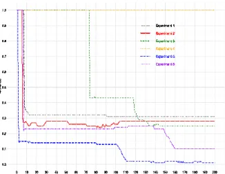
In the following figures, a sample of the most representative results are shown. Figure 2 shows the convergence speed of the tolerance of a single constraint, abritrarily chosen amongst one of these 10 constraints, upon several experiments. It exhibits that a limited number of steps is needed to reach a fixed point, according to the constraints strength. The tolerance converges to different values due to the fact that this particular constraint may be of more or less importance depending on the problem. It can be seen that the tolerance evolves by stages. This pattern can be explained by the fact that a Constraint Agent tightens its constraint only if the number of Inactive+Active data still matching the constraint with the new tolerance is sufficient. As this number steadily increases over time, the constraint can be tightened only when a certain threshold is reached. For example, for Experiment 2, the tolerance remains constant from step 105, which means that from this step on, the Constraint Agent related to this constraint decides at each iteration to leave the tolerance as is. However, the other constraints –not shown in this figure– are still able to adjust their tolerance.

Figure 3 shows the total number of data used against the simulation time, in iteration steps. This figure completes Fig. 2 and allows to see when the fixed point is actually reached. For example, for experiment 2, the fixed point is reached at 108 steps. The other constraints account for the 3 steps difference in reaching the fixed point between Fig. 2 and Fig. 3. Those results exhibit that less than 1% of the database is needed for the system to reach its fixed point and return a prediction to the user in less than 200 steps.

Figure 2: Convergence of a single constraint upon several experiments. Each colored

line represents one experiment

Figure 3: Convergence of the Inactive+Active dataset size upon several experiments

4.3 Prediction Results

In order to evaluate the AMAS algorithm performance to predict maize hybrid yield under environmental constraints, predicted yield values were compared to in-base recorded values. For each test, the set of constraints is automatically extracted from the database and is specific for each hybrid/trial couple.

Because our approach builds a new predictive model at each test, it is innately more related to adaptive data mining than model learning. Thus a classical cross

validation on a subset of data generally used to evaluate the latter model was considered as irrelevant. Instead, a thousand leave-one-out tests were carried out to produce a posteriori yield predictions.

Here is the modus operandi: At first, 200 individuals were randomly chosen, then, each individual underwent 5 randomly selected trials (a trial being selected only if containing the phenotype of the tested individual ), giving a thousand test cases. The significance of the samples was assessed by comparing the distribution of the yields from the samples and the entire database. 992 predictions out of 1000 data target have been tagged useful by the AMAS algorithm, meaning that the algorithm has converged on a yield prediction based on a dataset of a size greater than 9. The accuracy of the predictions has been evaluated with a special distinction on predictions considered as highly relevant by the AMAS algorithm: For each yield prediction an index of reliability is provided. This index is given by the ratio of the predicted yield standard deviation (SD) to the values of the predicted yields within the set of non-target data. A SD less than 10% of predicted value is considered highly relevant.

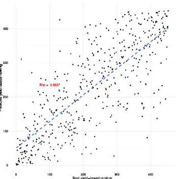
Pearson correlation is acknowledged to be the best way to evaluate the prediction accuracy [23] [24] [25]. In our tests, Pearson correlation between predicted and real yield/data is 0.67. Pearson correlation on the ranks of the target data gives Spearman correlation which, regarding the goal of the project to select the more valuable hybrids, is very interesting to calculate. In our tests, Spearman correlation between predicted and real yield/data is 0.65.

When carried on the 452 most reliable AMAS predictions (according to their SD), the Pearson and Spearman correlations are 0.79 and 0.78, respectively. Although based on a few target data, these first results have been considered very promising by the seed-breeders partnering the project as they are in the expected range according to state-of-the-art models. Due to confidentiality of agronomic data, we only present in Fig. 4 the non-parametric performance of AMAS prediction based on the 452 high confidence results, i.e. distribution of predicted yields regarding in-base recorded yields.

Figure 4: Distribution of predicted yields against recorded actual yields

5 Conclusion

This paper has presented an approach to overcome the lacks of the traditional statistical approaches for phenotypic prediction. This approach is based on a Multi-Agent System which aims at predicting the value of a phenotypic trait of a given hybrid in given environmental conditions. Choices made when modeling these data (gathered from domain experts, i.e. breeders and meteorologists) enable to consider them as equally important and to associate an agent with each one of them. A prediction is seen as seeking a solution able to satisfy the constraints imposed on the different variables defining the hybrid and environment targeted, and therefore imposed on the agents representing these variables.

By self-adjusting a tolerance on its constraint, each agent participates in the collective search of the solution, until trust and quality levels are found globally acceptable.

The contribution of this work is twofold: first, the choices made when modeling the problem enable to consider noisy or missing data, the self-adaptive algorithm produced by the AMAS functions like a heuristic to efficiently explore the solution space; and, secondly, it is one of the rare algorithms able to predict the G×E potential of a plant by considering both genetic and environmental data which are not already present in the subset of data used for calibrating the model [26].

Therefore our model appears to provide tangible solutions to those main issues, giving hope to improve genomic selection.

6 Acknowledgements

This work is part of the GBds (Genomic Breeding decision support) project funded by the French FUI (Fonds Unique Interministeriel) and approved by Agri Sud-Ouest Innovation (competitive cluster for the agriculture and food industries in southwestern France). We would like also to thank our partners in this project (Ragt 2n, Euralis and Meteo France) and Daniel Ruiz from the IRIT laboratory for his help concerning data analysis. This project is cofunded by the European Union which is involved in Midi-Pyrenees through the European Regional Development Fund.

7 Disclosure

Part of this article has been previously published in the 8th _{International Conference}

on Practical Applications of Computational Biology & Bioinformatics (PACBB 2014), Volume 294 of the series Advances in Intelligent Systems and Computing pp 1-8, DOI: 10.1007/978-3-319-07581-5_1

References

[1] Food and Agriculture Organization: The State of Food and Agriculture Food Systems 2013 Food Systems for Better Nutrition. Rome: FAO; 2013.

[2] Lorenz AJ, Chao S, Asoro FG, Heffner EL, Hayashi T, Iwata H, et al. Genomic Selection in Plant Breeding. In: Advances in Agronomy. Vol. 110. Elsevier; 2011. p. 77–123.

[3] Zhang Z, Ober U, Erbe M, Zhang H, Gao N, He J, et al. Improving the Accuracy of Whole Genome Prediction for Complex Traits using the Results of Genome Wide Association Studies. PLoS ONE. 2014 Mar; 9(3):e93017.

[4] Meuwissen TH, Hayes BJ, Goddard ME. Prediction of Total Genetic Value Using Genome-wide Dense Marker Maps. Genetics. 2001 Apr;157(4):1819-1829.

[5] Yu J, Pressoir G, Briggs WH, Vroh Bi I, Yamasaki M, Doebley JF, et al. A Unified Mixed-model Method for Association Mapping that Accounts for Multiple Levels of Relatedness. Nature Genetics. 2006 Feb;38(2):203-208. [6] Stich B, Mohring J, Piepho HP, Heckenberger M, Buckler E., Melchinger AE.

Comparison of Mixed-model Approaches for Association Mapping. Genetics. 2008 Feb;178(3):1745-1754.

[7] Beló A, Zheng P, Luck S, Shen B, Meyer DJ, Li B et al. Whole Genome Scan Detects an Allelic Variant of FAD2 Associated with Increased Oleic Acid Levels in Maize. Molecular Genetics and Genomics. 2008 Jan; 279(1):1-10. [8] Harjes CE, Rocheford TR, Bai L, Brutnell TP, Kandianis CB., Sowinski SG. Et

al. Natural Genetic Variation in Lycopene Epsilon Cyclase Tapped for Maize Biofortification. Science. 2008 Jan;319(5861):330-333.

[9] Whittaker JC, Thompson R, Denham MC. Marker-assisted Selection using Ridge Regression. Annals of Human Genetics. 1999 Jul;63(4):366-3666. [10] Bernardo R, Yu J. Prospects for Genomewide Selection for Quantitative Traits

in Maize. Crop Science. 2007;47(3):1082.

[11] Schaeffer LR. Strategy for Applying Genome-wide Selection in Dairy Cattle. J Anim Bree. Genet. 2006 Aug;123(4):218-223.

[12] Gerstein MB, Lu ZJ, Van Nostrand EL, Cheng C, Arshinoff BI, Liu T et al. Integrative Analysis of the Caenorhabditis Elegans Genome by the

[13] Meyer PE, Kontos K, Lafitte F, Bontempi G. Information-theoretic Inference of Large Transcriptional Regulatory Networks. EURASIP Journal on Bioinformatics and Systems Biology. 2007;2007:1-9.

[14] Robertson P, Shrobe H, Laddaga R, editors. Self-Adaptive Software. vol. 1936 of Lecture Notes in Computer Science. Berlin Heidelberg: Springer; 2001. [15] Salehie M, Tahvildari L. Self-adaptive Software: Landscape and Research

Challenges. ACM Transactions on Autonomous and Adaptive Systems. 2009 May;4(2):1-42.

[16] Di Marzo Serugendo G, Gleizes MP, Karageorgos A. editors. Self-organising Software: From Natural to Artificial Adaptation. Natural computing series. Heidelberg; New York: Springer; 2011.

[17] Wurtz RP. Organic Computing. Berlin: Springer; 2008.

[18] Kouvelas A, Papageorgiou M, Kosmatopoulos EB, Papamichail I. A Learning Technique for Deploying Self-tuning Traffic Control Systems. IEEE; 2011. p. 1646–1651.

[19] Weyns D, Brueckner SA, Demazeau Y, editors. Engineering Environment-Mediated Multi-Agent Systems. Vol. 5049 of Lecture Notes in Computer Science. Berlin, Heidelberg: Springer; 2008.

[20] Ferber J. Multi-Agent Systems: an Introduction to Distributed Artificial Intelligence. Harlow: Addison-Wesley; 1998.

[21] Capera D, Georgé JP, Gleizes MP, Glize P. The AMAS Theory for Complex Problem Solving based on Self-organizing Cooperative Agents. In: WETICE; 2003. p. 383–388.

[22] Ilin A, Raiko T. Practical Approaches to Principal Component Analysis in the Presence of Missing Values. J Mach Learn Res. 2010 Aug;11:1957-2000. [23] Albrecht T, Auinger HJ, Wimmer V, Ogutu JO, Knaak C, Ouzunova M et al.

Genome-based Prediction of Maize Hybrid Performance Across Genetic Groups, Testers, Locations, and Years. Theoretical and Applied Genetics. 2014 Jun;127(6):1375–1386.

[24] Heslot N, Yang HP, Sorrells ME, Jannink JL. Genomic Selection in Plant Breeding: A Comparison of Models. Crop Science. 2012;52(1):146.

[25] Meuwissen TH, Goddard ME. Prediction of Identity by Descent Probabilities from Marker-haplotypes. Genetics Selection Evolution. 2001;33(6):605. [26] Heslot N. Akdemir D, Sorrells ME, Jannink JL. Integrating Environmental

Covariates and Crop Modeling into the Genomic Selection Framework to Predict Genotype by Environment Interactions. Theoretical and Applied Genetics. 2014 Feb;127(2):463-480.