To cite this version :
Belgacem, Najib
and Prat, Marc
and Pauchet, Joël Coupled continuum
and condensation-evaporation pore network model of the cathode in
polymer-electrolyte fuel cell. (2017) International Journal of Hydrogen
Energy, Vol. 42 (n° 12). pp. 8150-8165. ISSN 0360-3199
O
pen
A
rchive
T
OULOUSE
A
rchive
O
uverte (
OATAO
)
OATAO is an open access repository that collects the work of some Toulouse researchers
and makes it freely available over the web where possible.
This is an author’s version published in :
http://oatao.univ-toulouse.fr/19954
Official URL :
https://dx.doi.org/10.1016/j.ijhydene.2017.01.184
Any correspondence concerning this service should be sent to the repository administrator :
Coupled continuum and condensatione
evaporation pore network model of the cathode
in polymer-electrolyte fuel cell
Najib Belgacem
a,b,c, Marc Prat
a,b,**, Joel Pauchet
c,*aINPT, UPS, IMFT (Institut de M!ecanique des Fluides de Toulouse), Universit!e de Toulouse, All!ee Camille Soula,
F-31400 Toulouse, France
bCNRS, IMFT, F-31400 Toulouse, France c
Univ. Grenoble Alpes, CEA LITEN, DEHT, 17 Rue Martyrs, F-38054 Grenoble, France
a r t i c l e
i n f o
Keywords:
Pore Network Model Condensationeevaporation Gas diffusion layer Rib-channel PEMFC
Continuum e PNM coupled model
a b s t r a c t
A model of the cathode side of a Proton Exchange Membrane Fuel Cell coupling the transfers in the GDL with the phenomena taking place in the cathode catalyst layer and the protonic transport in the membrane is presented. This model combines the efficiency of pore network models to simulate the liquid water formation in the fibrous substrate of the gas diffusion layer (GDL) and the simplicity of a continuum approach in the micro-porous layer (MPL). The model allows simulating the liquid pattern inside the cathode GDL taking into account condensation and evaporation phenomena under the assumption that the water produced by the electro-chemical reactions enters the MPL in vapor form from the catalyst layer. Results show the importance of the coupling between the transfers within the various layers, especially when liquid water forms as the result of condensation in the region of the GDL fibrous substrate located below the rib.
Introduction
Proton Exchange Membrane Fuel Cell (PEMFC) is considered as a key alternative to thermal engines for transport application, allowing no use of oil fuels and no emission of greenhouse gases. Numerous studies have been conducted in the last thirty years to increase its performance and durability, and reduce its cost, which are the three main bottlenecks to be
solved to ensure the mass market development of this solu-tion. Water management remains up-to-date a major limiting factor to performance and durability of PEMFC, see for instance Ref. [1]. Inside the Membrane Electrode Assembly (MEA) a trade-off is to be found between drying and flooding. Drying occurs when the membrane and/or the ionomer in the active layers do not contain enough water to ensure good proton conductivity, whereas flooding occurs when too much
* Corresponding author.
** Corresponding author. INPT, UPS, IMFT (Institut de M!ecanique des Fluides de Toulouse), Universite! de Toulouse, All!ee Camille Soula, F-31400 Toulouse, France.
E-mail addresses: [email protected] (M. Prat), [email protected] (J. Pauchet).
liquid water is present inside the MEA and reduces the gas access to the catalytic sites. In addition to increasing the performance, a controlled water management also allows increasing the durability of PEMFC as some degradation mechanisms are linked to the presence of liquid water and/or to the level of water vapor partial pressure inside the catalyst layer, see for instance Ref.[2].
Water management is closely linked to the operating con-ditions of the PEMFC (temperature, pressure and hydration of the gases, steady-state or transient…) but also to the properties of the layers used in the MEA, gas diffusion layer, catalyst layer and membrane. The multiple and conflicting functions of these layers (electrical and thermal conduction, gas diffusion and liquid water removal) and their coupling, see for instance Ref.[3], make however complex their optimization by semi-empirical trial and error test procedures. The development of more descriptive and predictive numerical simulation tools is necessary to better understand water management inside the MEA and its link to the properties of the layers. This is mandatory to progress towards “design” tools.
Important developments have been carried out in this domain for several years, such as the modeling of the MEA with more and more sophisticated representations of the various layers, see for instance Ref. [4], or the progressive consideration of the coupling between electrical, fluidic and thermal transports[5]. In these models, see also Ref.[6], the two-phase transport is based on the classical continuum approach to porous media. These models have allowed mak-ing progress in the understandmak-ing of the transfers within the PEMFC. However, the relevance of this approach has been questioned, i.e. Ref.[7], because of the capillary regime pre-vailing in the gas diffusion layers (GDL) and the obvious lack of length scale separation (only a few pores over the thickness of the fibrous substrate of the GDL). The latter is generally a two-layer system resulting from the assembly of a fibrous sub-strate, referred to as the diffusion medium (DM), and a micro-porous layer (MPL).
As an alternative, Pore Network Model (PNM) has been applied to PEMFC. PNM is well adapted to model the capillary regime, especially in thin layers such as the DM of the GDL, e.g. Ref.[8], as well as the more complex cases where the wettability is mixed (mixed refers here to situations where hydrophilic pores and hydrophobic pores coexist in the DM), e.g. Refs.[9,10]. For this reason, the use of PNM has up-to-date mainly focused on the DM even if some developments have also been conducted for the Cathode Catalyst Layer (CCL), e.g. Ref.[11]. To our knowledge, PNM has not been applied to the micro-porous layer (MPL) of the GDL, at least as a tool of simulation directly at the scale of the pore network of a MPL. However, results obtained from PNM simulations are exploited for example in Ref.[12]to study the optimal thick-ness of the MPL. For this reason, PNM is used in the present work to model the liquid water formation in the DM.
Regarding the simulation of two-phase flows in the DM with PNM, one can distinguish the simulations performed in conjunction with ex-situ experiments from the more chal-lenging simulations aiming at predicting the liquid water distributions within the GDL in an operating fuel cell. Regarding the former, recent works have confirmed that a standard invasion percolation algorithm is well adapted to
describe the ex-situ situation where typically liquid water is injected from one side in a dry GDL[13,14], at least when the medium is hydrophobic.
The situation regarding the in-situ case is much less clear. In a majority of works, see references in[15], a scenario similar to the ex-situ case is considered. Namely, liquid water enters the GDL in liquid phase from the CCL. This situation of liquid water injection is referred to as the injection scenario.
However, a completely different option is considered in Ref. [15]where it is assumed that water enters the GDL in vapor form. According to the scenario considered in Ref.[15], liquid water can form in the DM as a result of the condensa-tion of the water vapor in the colder zones of the DM (essen-tially in the region of the DM below the ribs). This situation of liquid water condensation is referred to as the condensation scenario. An important feature of the model in Ref. [15]is therefore to take into account the temperature variations within the GDL. The liquid distribution is significantly different between the two options. As discussed in Ref.[15], the condensation scenario is in good agreement with several experimental results presented in Refs. [16,17], noting that these experiments are performed at temperatures close to the standard operating temperature of PEMFC (~80!C). As in the
experiments [16], the simulations show that the GDL is completely dry at sufficiently low current density and/or relative humidity in the channel. As in the experiments[16], a strong ribechannel separation effect is observed when liquid water is present, i.e. the liquid water accumulates in the re-gion below the rib and no water is observed bellow the channels. As in the experiments[17], the saturation along the DM thickness increases from CCL to rib/channel area, whereas this saturation typically decreases according to the simulations based on the liquid injection scenario, e. g. Ref.
[18]. The impact of average current density and channel relative humidity on saturation profiles are also consistent with the experimental results reported in Ref.[17]. Despite all these elements showing several points of good agreement between the experiments and the simulations, we do not claim that the PNM presented in Ref. [15], is adapted to describe all the situations encountered in PEMFC as regards the liquid water formation and displacement in the GDL. For instance, it could be not sufficient when the operating tem-perature is significantly colder than 80!C or when the relative
humidity in the channel is close to 100%. Further work is needed to test or improve the model for those conditions. Nevertheless, based on the overall good agreement between the condensationeevaporation PNM [15,19] and several experimental observations as mentioned above, the model presented in what follows adopts the same option as in Ref.
[15]as regards the computation of the liquid water formation. It can be noted that the consideration of condensation phenomenon in a discrete approach as a key aspect of liquid water in the DM is not restricted to the works presented in Refs.[15,19]. A condensation algorithm is also presented in Refs. [20,21]and the conclusion is that condensation has a significant influence of the liquid distribution. However, the model is different from the one proposed in Ref.[15]. This is actually not a PNM but a somewhat different discrete approach. In contrast with the model presented in Ref.[15], only simulations in 2D discrete structures are presented in
Refs.[20,21], and liquid injection is considered together with condensation. Thus, the fact that the GDL can be completely dry is not pointed out. The condensation algorithm is completely different and relies on a coupling with a contin-uum model to compute the sourceesink terms in the GDL associated with condensation and evaporation phenomena. By contrast, all the phenomena are directly computed at the pore network scale in the DM (which is referred to as the fibrous substrate (FS) in Refs.[20,21]), in our model. We can also mention the recent numerical work presented in Ref.[22]
on the impact of the MPL. This work is based on a two-dimensional dynamic pore network taking into account the condensation evaporation phenomena. There is, however, no coupling with the electrochemical phenomena in the CCL.
Compared to the model presented in Ref.[15], the objective of the present article is to improve the modeling of the cath-ode by essentially coupling the PNM presented in Ref.[15]with the phenomena occurring in the adjacent layers, namely the MPL, CCL and the membrane and in particular with the elec-trochemical reactions taking place in the CCL.
In Ref.[15], only the DM is considered and important data such as the current density and heat flux distributions at the DM inlet are not computed but are imposed as input data. By introducing the coupling, these data will be outputs of the computations. Another important objective is to evaluate the impact of the coupling on the results obtained using the simpler approach proposed in Ref.[15]. As we shall see the coupling is performed by coupling the PNM describing the transport phenomena and the water formation in the DM, with continuum models for the MPL, and with the phenomena taking place in the CCL.
Developing mixed approaches coupling PNM and contin-uum models is not a novelty in the context of PEMFC. The previously mentioned work presented in Ref. [21] is an example. More recently, on can refer to the works presented in Ref. [23], where three different coupling methods are dis-cussed. The pore network is however only 2D and again it is assumed that water enters in liquid form into the GDL. As a result the liquid distribution in the DM depicted in this paper (see Fig. 10 in Ref.[23]) has nothing to do with the liquid dis-tributions presented in Ref.[15]. This also holds for the liquid water distributions computed by the same group in Ref.[24]. Interestingly, the temperature in Ref.[24]is quite low (25!C),
much below the standard operating temperature (~80 !C)
considered in Ref.[15]. A coupled continuum-PN models is also presented in Ref. [25]. This model couples a three-dimensional PNM in the GDL to continuous models in the other layers for anode and cathode sides. However, this model is limited to isothermal situations and the injection scenario in the DM (no MPL is modeled) for which the injection points at the interface GDL/CCL are inputs of the models. The condensation phenomenon is completely ignored.
The paper is organized as follows. The fuel cell cathode sub-domain of interest is described in Section “Cathode unit cell”. The physical models used in the different layers are presented in Section “Transport phenomena in GDL and associated boundary conditions (dry condition)”. The pore network approach for computing the various transport phe-nomena in the DM is presented in Section “Pore network approach of transport in DM”. Section “Continuum approach
of transport in MPL” describes the continuum model used for the MPL. The CCL and membrane discrete representations are presented in Section “Catalyst Layer and membrane”. The coupling procedure is described in Section “Coupling GDL with CCL and membrane”. Results are presented and discussed in Section “Results and discussion”. Finally conclusions are dis-cussed in Section “Conclusions”.
Cathode unit cell
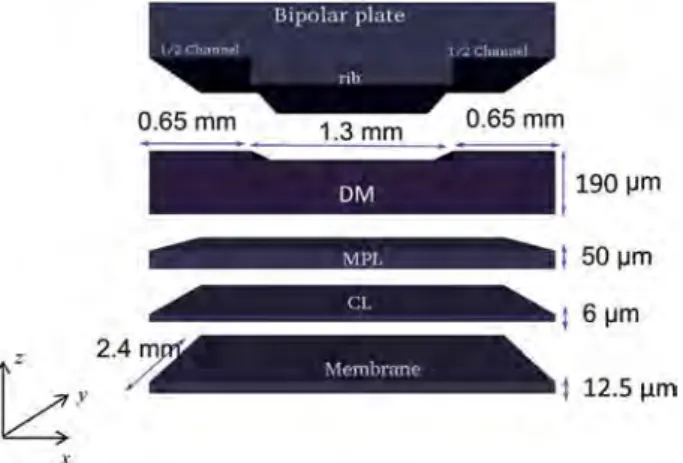
As depicted inFig. 1, our model is developed at the rib/channel scale, which means over a domain adjacent to one rib and two half-channels. The corresponding domain is referred to as a cathode unit cell. The domain includes the GDL (DM and MPL), the cathode catalyst layer (CCL) and the membrane. As we shall see transport equations are discretized over the GDL (MPL þ DM) only, whereas computational cells located in the membrane and the (CCL) are used in the coupling procedure. The domain is 3D with extension into the y direction (flow direction in the channel). It can be noted that this feature is not useful when only single phase transports are considered in the cathode as the boundary conditions applied along y are uniform. Nevertheless, even with uniform boundary condi-tions in y direction, this 3D extension is mandatory when liquid water is considered as connectivity properties of the liquid and gas phase at the pore network scale are different in 3D and in 2D[26].
The compressibility of the GDL is taken into account in our model as it has an influence on transfers below the rib and below the channel. As indicated inFig. 1, the thickness of the uncompressed GDL is 240 mm corresponding to the sum of the DM (190 mm) and of the MPL (50 mm), as for the SGL 25BC used as a reference GDL for this study (see SGL web site). The CCL has a thickness of 6 mm (typical of catalyst loading around 0.4 mgPt/ cm2) and the membrane is 12.5 mm in thickness (typical of
Nafion NR-211). The compression of the GDL below the rib (due to the clamping pressure) is set at 20% of the uncompressed DM (so 38 mm), as classically used in performance tests.
The unit cell is considered as the representative cell of a spatially periodic system. As a result, spatially periodic boundary conditions are applied on the lateral, front and back surfaces of the unit cell for each considered transport phe-nomenon (heat, electrical current, liquid water, vapor water,
and O2). These boundary conditions are thus not discussed
anymore in what follows where the focus is on the more important boundary conditions along the GDL/rib-channel interface and along the MPL/CCL interface.
Transport phenomena in GDL and associated
boundary conditions (dry condition)
Gas transport
As discussed in Ref.[15]and mentioned in the introduction, an important feature directly related to the assumption of the water entering in vapor phase into the GDL is that the GDL can be dry without any liquid water formation when the current density and/or the relative humidity in the channel are suffi-ciently low. For this reason, the case of the dry GDL is distin-guished from the case of the wet GDL.
For the dry condition only gas (water vapor, nitrogen and oxygen) is present in the GDL. The various transport mecha-nisms considered are summarized inFig. 2. Gas, thermal and electrical transfers are considered in the GDL (DM and MPL) under the following assumptions: i) nitrogen is a stagnant gas, ii) water vapor and oxygen diffuse in the pore space according to Fick's law. Assuming for the moment that the DM and MPL can be described as effective media (continuum approach), the diffusion problem is thus expressed as
JH2O ¼ $DH2O$VcH2O (1)
JO2 ¼ $DO2$VcO2 (2)
where JH2O, JO2are the molar fluxes (mol m$2s$1), cH2Oand cO2
are the molar concentrations (mol m$3
), and DH2Oand DO2are
the effective diffusion tensor of water vapor and oxygen respectively. The mass conservation of each species is expressed as,
V$JH2O¼0: (3)
V$JO2¼0: (4)
The above equations are solved using the following boundary conditions, summarized in Fig. 3. Assuming ideal gas behavior in the channel, the gas concentrations is imposed at the GDL/gas channel interface as a function of relative humidity (RH), oxygen partial pressure (PO2), nitrogen
partial pressure (PN2), gas temperature (T), and total pressure
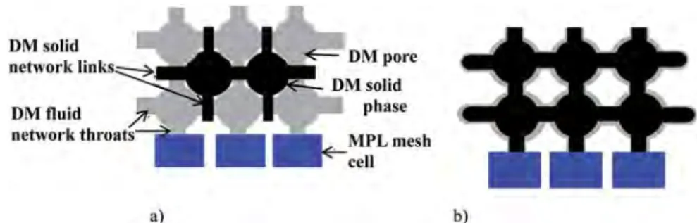
(Ptot) of gases in the channel, cH2O¼PH2O
RT (5)
cO2¼PO2
RT (6)
where
Ptot¼PH2OþPO2þPN2 (7)
PH2O¼xH2OPtot¼RH Psat (8)
PO2¼xO2Ptot (9)
Psat¼exp ! 23:1961 $ 3816:44 T $ 46:13 " (10) where xiis the mole fraction of species i.
Zero flux of vapor water and oxygen is imposed at the GDL/ rib interface.
At the GDL/CCL interface, it is assumed that only a fraction of the water flux jH2OCCLproduced by the electrochemical
re-actions in the CCL is transferred through the GDL (the com-plementary fraction is transferred through the membrane on the anode side). Thus, we impose on this interface,
jnetH2O; c¼ gmjH2OC (11)
Fig. 2 e Transfer mechanisms considered in the cathode GDL for the dry condition.
Fig. 3 e Summary of boundary conditions applied for the computations of transport phenomena in GDL. Spatially periodic boundary conditions are imposed on lateral sides of domain.
where the partition coefficient gmis typically in the range 0.5
e0.8 according to unpublished measurements performed at CEA/LITEN (LITEN is the laboratory to which one of the paper co-authors belongs). How jH2OCis computed is explained below
(see Eq.(26)). As mentioned in the introduction, it is assumed that the flux given by Eq.(11)is a water vapor flux (and not a liquid flux).
Similarly a flux condition is imposed at the GDL/CCL interface as regards the oxygen transport problem assuming no permeation through the membrane,
jO2;c¼jO2C (12)
How jO2Cis computed is explained below (see Eq.(25)). Heat transfer
The heat transfer is modeled according to Fourier's law
q ¼ $k$VT (13)
V$ q ¼ 0: (14)
where q, T, and k are the heat flux (W m$2), temperature (K),
and thermal conductivity tensor (W m$1 K$1) of the GDL respectively.
The boundary conditions are the following. The rib tem-perature is known. Thus T ¼ Tribis imposed at this interface.
The temperature is also imposed at the channel/GDL interface with Tchannel¼Tribþ DT where DT is an input data. Typically
DT ¼ 2e5 !C according to unpublished measurements
per-formed at CEA/LITEN. The heat flux is imposed at the GDL/CCL interface. Similarly as for the water flux it is assumed that only a fraction of the heat flux generated in the CCL is trans-ferred through the cathode GDL,
qnet;c¼ gqqC (15)
where the partition factor gqis also typically in the range 0.5
e0.8 according to unpublished measurements performed at LITEN. How qCis computed is explained below (see Eq.(27)). Electrical transport
The electron transport is computed thanks to Ohm's law
i ¼ $s$Vj (16)
V$i ¼ 0 (17)
where i, s, and j are the current density (A m$2), electrical
conductivity tensor (S m$1), and electronic potential (V)
respectively.
Zero flux on electrical potential (current density is zero) is imposed at the GDL/channel interface whereas the cur-rent density iribis imposed at the GDL/rib interface so that
the current density irib Srib¼ I where I is the total current
(Amps) measured at cell level (Sribis the surface area of the
rib). The electrical potential j is imposed at the GDL/CCL interface,
j¼ jC (18)
How jCis computed is explained below (see Eq.(36)).
Due to its fibrous structure, the DM is considered as an anisotropic and deformable medium. The MPL is isotropic and not deformable owing to its granular structure. Accordingly, the transport tensors above are supposed isotropic for the MPL and identical in the regions below the rib and below the channel, whereas for the DM, the coefficients of the tensors are different in the in-plane and through-plane directions as well as below the rib and the channel. Details are given in the
Appendix.
When the conditions are such that liquid water forms in-side the GDL, the GDL is said to be wet. The presence of the liquid water has an impact on the transport. How this impact is taken into account in the model is described in Section “Pore network approach of transport in DM”.
As explained below, the steady-state solution obtained when liquid water forms inside the GDL corresponds to a situation where a balance is reached between the condensa-tion rate and the evaporacondensa-tion rate at the boundary of each liquid clusters present in the DM. It turns out that liquid water never reaches the channel in the cases we considered. Therefore the formulation of the boundary condition at the GDL/channel interface is the same for a dry GDL and a wet GDL. As reported in previous studies, e.g. Ref. [27], more involved situations with droplet formation at the channel/ GDL interface exist but the corresponding situations (colder operating temperature, higher relative humidity in the chan-nel) are beyond the scope of the present model. Zero flux of liquid is imposed at the rib/GDL interface.
Pore network approach of transport in DM
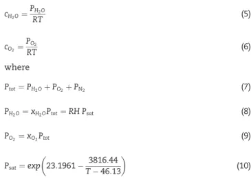
For simplicity, the interface between the two layers, namely the DM and the MPL, forming the GDL is assumed to be perfectly flat. The DM pore space is modeled as a 3D cubic pore network with a lattice spacing of 50 mm, leading to 52 pores in the rib/channel length, 5 in the thickness, and 52 in the di-rection of the channel (each pore is shown as gray cube in
Fig. 4). Each pore is cubic and is connected to six throats of square cross-section.
The throat sizes dtare randomly distributed in the range
[20 mm, 34 mm] according to a Weibull's law as in Refs.[9,10],
dt¼dtmin þ#dtmax$dtmin
$ % 2 6 4 ( $ dln ! l' ! 1 $ exp ! $1 d """ þexp ! $1 d ")g1 3 7 5 (19) with d¼0.1, g¼4.7, and l0is random number in the range [0,1].
Fig. 4 e Meshing of DM, MPL, catalyst layer, and membrane.
Then the size of each of the 52*52*5 cubic pores is specified as follows. Each pore diameter is first initialized to the maximum diameter of its neighboring throats, then adjusted to fit to the porosity (ε ¼ 0.8) of the DM. This adjustment is done by multiplying each pore diameter by the same factor.
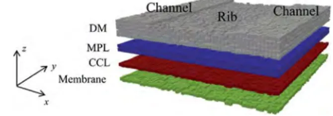
In the DM, two networks are actually created: the “fluid network” for the fluid transfers (in the pore space of the DM) and the “solid network” for the electrical and thermal transfers (in the fibers, binders… of the DM). The same number N of pores is considered for the solid and fluid networks. This is not fully consistent since as sketched in
Fig. 5it is more representative to locate the solid network nodes at positions different (shifted) from the nodes of the fluid network. As sketched inFig. 5b, collocated solid and fluid networks are actually considered in the modeling. Nevertheless, this assumption has no influence on the re-sults since no fluid/solid interactions are considered as regards the electrical and heat transfers. Diameters of the links in the solid network are also distributed according to a Weibull's law.
The transport phenomena in the DM are thus solved using the pore network approach, e.g. Ref.[8]. Since the diffusion transport in the gas phase, the heat and electric transports in the solid are basically governed by the same type of (diffusion) equation, the network formulation of the various transports is similar.
Conservation at each network node i (surrounded by s nodes) is expressed as
X
surrounding pores s
ji; s¼0 (20)
where ji,s is the flux into node i from surrounding pore s,
ji,s¼gi,s(Xs$Xi) where X is the variable associated with the
transfer mode considered (electrical, thermal transfers or gas diffusion).
The general formulation of the local conductance between nodes i and s is given as the harmonic average of the conductance gl i,sof the link between the two nodes, and those gpiand gpsof each half node:
1 gi;s¼ 1 gpi þ 1 gpsþ 1 gl i;s (21) where gp¼ b GXSp Lp (22) and gl¼ bGXSl Ll (23)
where Ll, Lp, Sl, Spare the local lengths L and cross-section sur-face areas S of the half nodes and of the link. These parameters are local and depend on the local structure of the GDL. GXis the
“conductivity” for the transfer considered (thermal and elec-trical conductivities, binary diffusion). It is the same every-where within the GDL volume. b is a fitting parameter that is adjusted to experimental results. Its value is different between in-plane and through-plane so as to take into account the anisotropy of the DM and below the rib and the channel so as to take into account the effect of the clamping pressure.
For electronic transfer, ji,s¼gi,s(js$ji), and GX¼ se, which
is the electrical conductivity of the carbon fibers (61,000 S m$1)
[28,29].
For heat transfer, ji,s¼gi,s(Ts$Ti), and GX¼ k, which is the
thermal conductivity of the carbon fibers (129 W m$1 K$1)
[28,29].
For gas diffusion, ji,s¼gi,s(Cs$Ci), and GX¼Dbin, which is the
binary coefficient diffusion of water vapor in air: 0.260 cm2s$1
[30], or Oxygen in air: Dbin¼ 3:2: 10$5
!
T
353
"1:5
1=p (m2s$1)
where p is the absolute pressure[20].
When liquid water is present in the DM, only the gas diffusion is modified by the presence of liquid water. Ac-cording to Burheim et al.[31], it would be interesting, however, to include in the future also the influence of liquid water on thermal effective conductivity. No gas diffusion can occur in the pores/throats fully invaded by the liquid whereas the local conductance gliqof the pore (and the throat) is modified as
gliq¼g ð 1 $ SÞ (24)
where S is the local water saturation of the pore and/or of the throat in the partially invaded throat or pore.
The values of the conductances and fitting parameters b from experimental results are given in theAppendix.
Continuum approach of transport in MPL
A direct pore network approach in the MPL implies considering a network much finer than in the DM since the pore sizes in the MPL are much smaller (typically on the order of 0.3e0.5 mm compared to 30e50 mm in the DM). For this reason and the fact that liquid water actually does not form in the MPL for the
conditions considered in the present paper, a standard finite volume technique on a cubic cartesian grid is used with the same spatial spacing as the lattice spacing of the DM (50 mm) in the in-plane directions and a mesh twice as finer in the through-plane direction (25 mm in mesh size) to solve the transports in the MPL. As sketched inFig. 4, this leads to two nodes in the thickness (~50 mm) of the MPL. Each computa-tional node of the MPL next to the DM is connected to one solid and to one fluid pore in the DM. We actually consider that the computational nodes in the MPL computational domain can be also regarded as “pores”, only to test if condensation can occur in the MPL “pores” (the quotation marks are here to recall that a “realistic” pore network description of the MPL would require a much finer discretization than considered here since the pore sizes in the MPL are orders of magnitude smaller than in the DM). It turns out that condensation does not occur in the MPL “pores” in the simulations performed (see Section “Results and
discussion”). Since the discretized forms of the transport equations are similar using the cubic pore network approach or a standard finite volume method, the transport phenomena in the MPL are in fact computed using the same formulations as the ones used for the DM, defining also local conductance for each of the transfer modes considered (electrical, thermal, gas diffusion, as for the DM). The MPL transport phenomena are solved with the same algorithm as for the DM (see below).
As for the DM, the different values of the conductances specified from experimental results are given in theAppendix. As sketched inFig. 5, each node of the MPL is connected to the corresponding throat/solid link of the GDL, for fluid and solid transfers. As the MPL and DM transport problems are discretized together over a single computational domain, the continuity of variables and fluxes at the DM/MPL interface is automatically satisfied.
Catalyst layer and membrane
A discrete representation of the catalyst layer and the mem-brane is used, using the same number of cells as the number of in-plane pores in the DM. Thus both layers are modeled as a collection of 52 % 52 in-plane cells connected to neighbor cells only in the through plane direction. Thus with only one node in the thickness (Fig. 4) and no in-plane transfers (on the ground that the thickness of these layers is very small compared to their in-plane extent). As a first step, this assumption is considered as sufficient as the primary aim of the model is a fine description of the DM even if coarse meshes are used for the other layers.
Each node of the CCL is connected to a fluid and to a solid node of the MPL, assuming the continuity of local gas con-centrations, temperature and current density.
Oxygen flux through the membrane (to reflect oxygen permeation) is an input of the model (set to zero in the sim-ulations presented in this work).
Coupling GDL with CCL and membrane
A key novel aspect compared to the model presented in Ref.
[15]is the coupling with the CCL. To solve the above transport
problems in the GDL, the distribution of jH2OC, jO2C, qCand jC
must be specified over the 52 % 52 cells of the CCL, which actually form the GDL/CCL interface. These 2D fields are not known a priori but are determined as the results of the coupling between the transport phenomena and liquid for-mation, if any, in the GDL and the electro-chemical phe-nomena occurring in the CCL. With the Oxygen Reduction Reaction (ORR) 1
2O2þ2Hþþ2e$/H2O as the baseline for the
cathode electrochemical behavior, the ORR oxygen con-sumption flux jO2C (mol s
$1m$2), water production flux j
H2OC
(mol s$1m$2), and heat generation q
C(W m$3) are computed
as a function of the current density distribution iC(x, y, 0)
within the CCL as jO2C¼ iC 4F (25) jH2OC¼ $iC 2F (26) qC¼!DH nF$ jC " iC (27)
where F is the Faraday constant (96,485 A mol$1), DH is the
ORR enthalpy ($242 kJ mol$1,[32]), n is equal to 2 considering
the ORR as a two-electron reaction.
The ButlereVolmer equation[33e35], written for the ORR at the cathode side, gives the relationship between the local current production rate at the CCL iC(A cm$2of catalyst) and
the local overpotential at the cathode hC(V): iC¼i0c ! exp!anF RThC " $exp ! $ð1 $ aÞnF RT hC "" (28) where R is the ideal gas constant (8.3 J mol$1K$1), The ex-change current density i0c(A cm$2) in Eq.(28)is expressed as: i0c¼n k0exp ! $A0 RT " . agO2 O2 /1$a. agH2O H2O /a (29) where aH2O, aO2 aH2 are the activities of water vapor, oxygen,
and hydrogen respectively (aH2O¼ PH2O Psat, aO2¼ PO2 Pref; aH2¼ PH2 Pref
where PH2O, PO2; PH2are the partial pressures of each gas, Psatis
the saturation vapor pressure at temperature T, Pref is a
reference pressure set at 1 bar).
The different parameters of the ButlereVolmer equation allow representing the behavior of the catalyst layer as a function of temperature, gas activities and over-potential. They are dependent of the properties of the catalyst layer, for instance the catalyst, carbon, and ionomer grades used, as well as the process applied to produce such catalyst layer. For the present study, the parameters are fitted on results from internal experiments [36] on given electrodes. This fitting leads to the values of k0(4.2 % 10$8m s$1), a (0.6), gO2(0.41), and
gH2O (2.04). The positive sign of gH2O can be surprising as
generally it is negative stating that i increases as aH2O
de-creases. This positive value of gH2Ois explained by the fact
that the catalyst layer description in the model presented here does not contain explicitly the protonic transfers which in-creases as aH2Oincreases. The positive value found by fitting to
experimental data allows taking into account this aspect and is consistent with the experimental increase of performance of the active layer with the relative humidity (RH).
The over-potential hCin Eq.(28)is related to the electrical
potential jCby
jC¼Erevþ hCþ fc (30)
where Erevis the thermodynamical reversible potential (V) and
fcis the protonic potential (V). The Nernst equation [37]is
used for the computation of the thermodynamical reversible potential: Erev¼DH $ TDS nF þ RT nFln . a12 O2aH2a$1H2O / (31) where DS is the ORR entropy ($44 J mol$1,[32]).
The protonic potential fc(V) at the interface between the
CCL and the membrane is a function of the current density through the membrane and expressed as
fc¼ faþRmiC (32)
where fais the protonic potential along the membrane on
the anode side, taken equal to zero for simplicity. This protonic potential at the anode side could be calculated (and no more used as an input parameter) with an anode elec-trochemical model, which could be a future extension of the current work. Rm is the resistance of the membrane
expressed as Rm¼hm/smwhere hmis the membrane
thick-ness and sm(S m$1) is the protonic resistance of the
mem-brane; smis modeled as a function of its water content l and
its local temperature[38]as,
sm¼ ð33:75l $ 21:41Þexp ! $1268 T " (33) where l is the number of water molecules per sulfonic group
[38].
l¼0:043 þ 17:81aH2O$39:85a2H2Oþ36a3H2O (34)
The ButlereVolmer equation (Eq. (28)) varies monoto-nously with h. We can thus define the inverse ButlereVolmer function as the function giving hc knowing iC. The Butler
eVolmer inverse function is denoted by g(iC). Thus
h¼gðiCÞ (35)
Thus, Eq.(31)can be expressed as
jC¼ErevþgðiCÞ þRmiC (36)
where, except for the very first iteration (see below), iC is
computed from the relationships
iC¼i ¼ $sMPLVjc$n (37)
where n is the unit normal vector at the CCL/MPL interface. The simulations aim at calculating the global electrical potential together with the distributions of electrical and protonic potentials, current density, O2, H2O (vapor and liquid,
if any), and T, as a function of the global current density for specified boundary conditions.
For each physical problem (mass, thermal and electrical transports) the mathematical system to be solved is of the form A(X)X ¼ B(X) where X contains the corresponding unknowns (temperature, gas concentrations, electrical potential, current
density in the GDL…), B(X) takes into account the boundary conditions (temperature and gas concentration in the channel, current density on the rib…) and A(X) is a matrix whose co-efficients notably depend on the conductances. The system is non-linear as for instance kinetic coefficients are function of gas concentration, themselves function of gas flux, and themselves function of current density. For this reason, an iterative method is necessary. This holds for the dry condition (no liquid in the assembly) as well as for the more involved wet condition (existence of liquid water in the DM).
Dry condition
The algorithm for the dry conditions is summarized inFig. 6. To start the iteration process, the current density i0and the
electrical potential j at the MPL/CCL interface are initialized imposing i0 ¼ I/Suc (S
uc is the in plane surface area of the
cathode unit cell) and j from the polarization curve U(i) (which is an input data) for the considered value of I. The heat flux produced by the ORR for the very first iteration is then calculated from the equation q0
¼i0(1.18$U(i)) whereas the
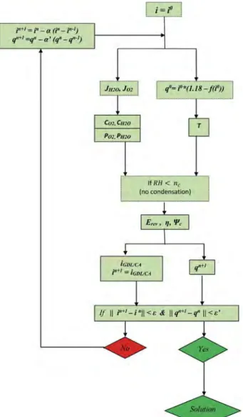
oxygen and water vapor fluxes at this interface are computed from Eqs.(11) and (12)combined with Eqs.(25) and (26). This gives the boundary condition to be applied for the computa-tion of the thermal, gas and electrical transfers inside the GDL. The latter gives the gas concentrations, temperature and electrical potential in the GDL, and especially at the MPL/CCL interface. This allows updating the current density and heat flux distributions at this interface. These distributions are then used as inputs for the following iteration. The current density is no more uniform due to the presence of the chan-nels and rib which affects the homogeneity of the transfers. The process is repeated until convergence on current density i and heat flux q is reached over the MPL/CCL interface. As indicated inFig. 6, convergence is considered to be reached when the Euclidean norm of the variations of i and q between two successive iterations is lower than some specified small parameters ε and ε0(taken equal to 10$3and 10$2respectively
in the simulations discussed in the next section).
As also indicated inFig. 6, it is useful to introduce under relaxation parameters, denoted by a and a0inFig. 6, to speed
up or stabilize the numerical procedure.
Wet condition
The modeling of liquid water formation and growth in the DM is a two-steps approach similar to the one described in Ref.
[15]: i) nucleation points, i.e. points where liquid water forms as a result of condensation, are identified, ii) the growth of the liquid clusters from the nucleation points is computed as a function of local conditions and local capillary forces, assuming that the growth is driven by capillary forces. Note that liquid water forming in the DM cannot flow from the DM into the MPL as the capillary entry pressure inside the MPL is much higher than the one inside the DM.
The specific treatment performed to account for sation can be summarized as follows. To identify if conden-sation occurs, a nucleation parameter ncis defined. In the
simulations presented in the next section, this parameter is set to 1 (a value greater than 1 would reflect a possible su-persaturation effect in the pore). Then after each iteration, the relative humidity field (RH ¼PH2O
Psat) is computed in each pore of
the DM (and the MPL) and compared to nc. The dry condition
corresponds to a situation where RH < ncin every pore after
each iteration until convergence. When this is not the case, the algorithm for wet condition is used.
Once the condition RH ) ncis reached, this means that there
is condensation in at least one pore of the GDL. As a result of condensation, liquid clusters can form and grow within the GDL. Liquid water formation occurs in addition to the other transfers (gas, thermal and electrical) and induces additional coupling as the local liquid saturation reduces the local gas diffusion and then can influence the gas concentration in the CCL and thus the local current produced. This means that the computation of the liquid pattern must be performed at each step of the iterative algorithm. This computation is performed keeping constant the other unknowns. This introduces an additional step compared to the dry algorithm.
Starting from the nucleation points, the liquid cluster growth is computed using the classical invasion percolation
(IP) algorithm[39,40]combined with the computation of the net mass flow rateP
neighboring poresJH2Oat the boundary of each
cluster. Note that the sizes of the throats in the through plane direction are multiplied by a factor 2 when applying the IP algorithm so as take into account the impact of the DM anisotropy on the liquid invasion. When Pneighboring pores JH2O>0
the condensation rate at the surface of the cluster is greater than the evaporation rate from this cluster and the cluster can grow according to IP rules. Otherwise the cluster is considered as having reached an equilibrium between condensation and evaporation and cannot grow any more.
The simulation stops once each cluster has reached a steady state (condensationeevaporation equilibrium). Note that new nucleation points, if any, are detected after each growth step.
The convergence criterion is not different than for the dry conditions and is based on the convergence of the spatial distributions of current density and heat flux over the MPL/ CCL interface.
The algorithm for the wet condition with liquid water forming as a result of condensation is summarized inFig. 7.
The whole software is written in Cþþ. This is an in-house code not using any commercial software or pieces of com-mercial software.
Results and discussion
To discuss the impact of the coupling between the transport phenomena in the various layers, which is a key new feature compared to the model presented in Ref.[15], solutions ob-tained using the coupling procedure are compared with so-lutions obtained without using the coupling procedure. The results presented below highlight when the coupling is ex-pected to have a significant influence on the results, and, on the contrary, when it can be expected to have a small influ-ence. Comparisons will be based on various transverse pro-files. Those profiles are determined at the MPL/CCL interface in the median x, z plane located in the middle of the cathode unit cell (seeFig. 3where this plane is shown).
In order to evaluate the interest of such coupling, simula-tions are performed for the dry as well as for the wet condi-tions, meaning without and with liquid water formation inside the GDL.
The non-coupled model used here is exactly the same as the coupled model described in the previous sections as regards the GDL and the boundary conditions at the GDL/rib, GDL/channel interfaces and lateral surfaces. The difference between the two models is that the catalyst layer model is not used in the non-coupled model. As the result, the current density distribution at the MPL/CCL interface is not computed anymore but given as an input. With this boundary condition, the other physical variables at the MPL/CCL interface are computed as for the coupled model. The same algorithms (Figs. 6 and 7), are actually applied in both cases. However, only one iteration is performed for the non-coupled model (to compute the various transport phenomena in the GDL for the given current density at the MPL/CCL interface) whereas the simulations are performed up to convergence for the coupled
Fig. 8 e Relative humidity distribution in a through-plane slice in the GDL (coupled model, i ¼ 0.6 A cm¡2,
RHchannel¼ 20%, dry condition, Trib¼ 80!C, DT ¼ 2!C,
PO2¼ 0.21 bar). The vertical scale is dilated for clarity.
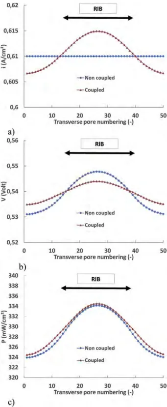
Fig. 9 e Distribution of the current density (a), electrical potential (b), and power density (c) at the MPL/CCL interface under dry condition, i ¼ 0.6 A cm¡2, RH
channel¼ 20%, Trib¼ 80!C, DT ¼ 2!C, PO2¼ 0.21 bar. Results obtained with the coupled model (red curves) are compared to the results obtained with the non-coupled model (blue curves). The transverse pore numbering corresponds to the position of the 52 pores in the DM network along the rib/channel direction in the median xz plane. (For interpretation of the references to colour in this figure legend, the reader is referred to the web version of this article.)
model (so as to also determine the current density distribution at MPL/CCL interface).
All the simulations presented and discussed below are performed for temperature Trib ¼ 80 !C and gas
pressure ¼ 1.5 bar. The oxygen concentration imposed in the channel in all simulations corresponds to PO2¼0.21 bar.
Dry condition
Dry conditions are typically obtained when the current density and or the relative humidity in the channel are sufficiently low. As illustrated inFig. 8, this is for example the case in our simu-lations, when the relative humidity RH in the channel is equal to 20% and the average current density is i ¼ 0.6 A cm$2. Although
the local relative humidity is everywhere lower than 1 in this example, it can be seen fromFig. 8that the relative humidity is higher in the central region of the GDL below the rib. This pre-figures the most likely place of condensation when RH and/or i will be increased (see below the “Wet condition”section).
The corresponding current density profile at the MPL/CCL interface computed with the coupled model is depicted in
Fig. 9a. This profile is smooth and characterized by a slight maximum below the rib. This indicates that the limiting factor for performance is most probably due to electrical transfers inside the GDL rather than to gas species diffusion transfers.
As can be seen fromFig. 9, the local current density and the electrical potential distributions at the MPL/CCL interface for this case are nearly the same between the non-coupled and the coupled models. This suggests that the coupling between GDL and CCL is not a first order issue when considering the computation of the transfers at the cathode, at least when the current density and relative humidity in the channel are suf-ficiently low. This is confirmed by the power density profiles shown inFig. 9c. The average power density is 328.7 mW cm$2
with the non-coupled model and 329.3 mW cm$2 with the
coupled model. This is consistent with the fact that in both cases the current density profiles are nearly the same, so are the heat fluxes, gas concentrations, and electrical potentials.
As can be seen fromFig. 10, increasing the mean current density from 0.6 A cm$2to 1.4 A cm$2in order to enhance the
differences between the two models first leads to higher values of the local relative humidity than at i ¼ 0.6 A cm$2(maximum
is 0.45 instead of 0.33) but still lower than 100% everywhere in
Fig. 10 e Relative humidity distribution in a through-plane slice in the GDL (coupled model, i ¼ 1.4 A cm¡2,
RHchannel¼ 20%, Trib¼ 80!C, DT ¼ 2!C, PO2¼ 0.21 bar, dry
condition). The vertical scale is dilated for clarity.
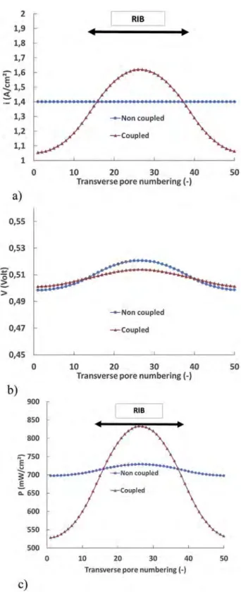
Fig. 11 e Distribution of the current density (a), electrical potential (b), and power density (c) at the MPL/CCL interface under dry condition, i ¼ 1.4 A cm¡2, RH
channel¼ 20%,
Trib¼ 80!C, DT ¼ 2!C, PO2¼ 0.21 bar. Results obtained with the coupled model (red curves) are compared to the results obtained with the non-coupled model (blue curves). The transverse pore numbering corresponds to the position of the 52 pores in the DM network along the rib/channel direction in the median xz plane. (For interpretation of the references to colour in this figure legend, the reader is referred to the web version of this article.)
the GDL. The comparison betweenFigs. 8 and 10show that the local relative humidity is again higher in the central region below the rib but it seems that the maximum is now right below the rib (Fig. 10) rather than at the MPL/CCL interface (Fig. 8). As shown in Fig. 11a, the current density profile computed with the coupled model is still smooth with again a maximum below the rib. So the limiting factor is suspected to be also the electrical transfers. As depicted in Fig. 11b, the electrical potential profile is not so different between the two models but the current density and the power density profiles are modified. The average power density is 712 mW cm$2with
the non-coupled model against 673 cm$2 with the coupled
model (so roughly 5% lower), showing that the increase of the average current density increases the non-uniformities within the MEA. Thus, the coupling between the GDL and the CCL appears to be more and more important and necessary as the average current density is increased.
Wet condition
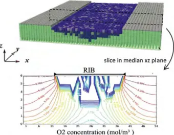
As can be seen fromFig. 12, a significant fraction of the DM pore space is invaded by liquid water as a result of conden-sation when the relative humidity is set equal to 90% in the channel and the average current density set equal to 1.4 A cm$2.
As can be seen fromFig. 13, the current density profile then changes significantly. A significant minimum appears below the rib, meaning that the dominant limiting factor for perfor-mance is not the electrical transfer in the GDL anymore as for the dry case, but the diffusion transfer of the gaseous species. This can be attributed to the presence of liquid water appearing below the rib. This liquid region reduces the region below the rib available for the oxygen transport and thus reduces the oxygen diffusion through the GDL (as illustrated inFig. 12).
As shown inFig. 13, the local current density, the electrical potential, and the electrical power density profiles at the MPL/ CCL interface are completely different between the coupled
and the non-coupled models for this wet condition. As illus-trated inFig. 14, this is mainly due to the fact that the liquid water distribution is different in both cases with a greater amount of liquid water close to the CCL with the non-coupled model. This can be explained by the fact that in the
non-Fig. 12 e Impact of liquid water (in blue) produced by condensation on oxygen diffusion distribution in GDL (coupled model, wet condition, i ¼ 1.4 A cm¡2, RH
channel¼ 90%
Trib¼ 80!C, DT ¼ 2!C, PO2¼ 0.21 bar). (For interpretation of
the references to colour in this figure legend, the reader is referred to the web version of this article.)
Fig. 13 e Distribution of the current density (a), electrical potential (b), and power density (c) at the MPL/CCL interface under wet condition, i ¼ 1.4 A cm¡2, RH
channel¼ 90%,
Trib¼ 80!C, DT ¼ 2!C, PO2¼ 0.21 bar. Results obtained with
the coupled model (red curves) are compared to the results obtained with the non-coupled model (blue curves). The transverse pore numbering corresponds to the position of the 52 pores in the DM network along the rib/channel direction in the median xz plane. (For interpretation of the references to colour in this figure legend, the reader is referred to the web version of this article.)
coupled model, the current density profile at the MPL/CCL interface is uniform and thus the heat flux is also uniform, whereas the current density and heat flux are strongly non-uniform with the coupled model and significantly lower below the rib than in the non-coupled case. As a result, the vapor flux injected in the region below the rib is much greater with non-coupled model since this flux is directly propor-tional to the current density (Eq. (26)). The power density profiles are also different in both cases, with an average power density around 561 mW cm$2with the non-coupled model
and 750 mW cm$2with the coupled one (so roughly þ 35%).
This is a strong indication that the coupling with the CCL must be taken into account in order to compute the transfers when liquid water forms inside the GDL.
Interestingly the fact the local current density inside the MEA is different between the regions located below the rib and below the channel is consistent with the experimental mea-surements reported in Refs.[41,42].
As exemplified inFig. 14, the coupled model and the non-coupled models both lead to the typical liquid distribution already discussed in Ref.[15]characterized by a strong separation between the region below the rib, where the liquid water accu-mulates, and the region below the channel, which remains dry.
Conclusions
In this paper, a model of a PEMFC cathode is proposed, coupling the electro-chemical phenomena taking place in the catalyst layer with a Pore Network Model (PNM) for computing the transfers and the liquid water formation in the diffusion medium (DM) of a GDL and a continuum approach in the MPL. A distinguishing feature of PNM is to model the liquid water formation by condensation in the DM and to assume that the water formed in the CCL enters the GDL in vapor form. For the conditions studied, the present study indicates that liquid water formation due to condensation takes place in the region of the GDL below the rib confirming the results obtained in Ref.[15]with a non-coupled model. The results show that it is important to take into account the coupling with the CCL as the current density profile at the CCL/GDL interface is essen-tial for simulating the performance of the MEA. This is crucial when liquid water appears in the GDL because of the impact of the liquid water formation on the gas transport.
More generally, the study illustrates that correctly dicting the liquid water pattern is very important for pre-dicting the transfers and the performance of the MEA. Fig. 14 e Liquid water (in blue) distribution in the DM under wet condition for the coupled (a) and non-coupled (b) models; i ¼ 1.4 A cm¡2, RH
channel¼ 90%, Trib¼ 80!C, DT ¼ 2!C, PO2¼ 0.21 bar. (For interpretation of the references to colour in this figure legend, the reader is referred to the web version of this article.)
Consequently, as the two-phase patterns are fully different between the condensation scenario in the GDL considered here (strong separation effect with the liquid water located in the central region below the rib) and the more classical sce-nario of injection directly in liquid phase (not leading typically to the channelerib separation effect), there is still a need to better understand the water formation in the GDL. For example, we surmise that the condensation scenario consid-ered in the present paper is well adapted to the situations where the operating temperature is sufficiently high (~80!C)
since as mentioned in the introduction it leads to several re-sults in good agreement with experiments for this condition. For sufficiently low operating temperatures, considering that all the produced water enters the GDL in vapor phase might be a too restrictive assumption and mixed scenario combining condensationeevaporation with liquid injection could be an interesting option. Also, we have not considered situations where the liquid water can reach the channel (the relative humidity in our simulation is always lower than 100% in the channel). This case would also deserve to be studied.
The present model needs improvements also for the con-ditions to which it is a priori well adapted. For instance, the discretization of the MPL must be refined as well as in the CCL with the consideration of the in-plane transport. The impact of liquid water on GDL thermal conductivity, the consider-ation of phase change phenomena on the thermal transport in the GDL are also to be included in the model for better de-scriptions. Here, the objective was more modest. It was to introduce a methodology for the coupling and to evaluate the impact of the latter.
Acknowledgements
This research has received funding from the European Union's Seventh Framework Programme (FP7/2007-2013) for the Fuel Cells and Hydrogen Joint Technology Initiative under grant agreement n!
303452, “IMPACTdImproved Life-time of Automotive Application Fuel Cells with ultra-low Pt-loading”.
Appendix
Transport parameters of the GDL model are fitted by comparing results from the model to available measure-ments on SGL 25 BA (DM only) and SGL 25BC (DM and MPL). When the desired data are not found in the litera-ture, in-house measurements and/or results on other GDL are used. This fitting allows finding, for each physical transfer:
*the “tortuosity” coefficients b of the DM, under the rib and under the channel, in-plane (denoted with subscript //) and through-plane (denoted with subscript t)
*the conductances g of the MPL considered as isotropic and not compressible
These parameters are given in the tables below with also a comparison of effective properties as modeled and as measured on the DM/MPL assembly to check the consistency of the model.
Table 1 e Coefficients used for modeling the gas transfer. (*) evaluation from Ref. [43] with Dbin¼ 0.35 cm2s¡1.
Gas diffusion Rib Channel
// t // t
DM Tortuosity b ($) 1 0.4 1 0.4
MPL g (m3s$1) 1.9 % 10$9 1.9 % 10$9 1.9 % 10$9 1.9 % 10$9
SGL 25BC Deff/Dbin(Experiments) e e e ~0.17 (*)
Deff/Dbin(Simulation) 0.5 0.08 0.6 0.15
Table 2 e Coefficients used for modeling the electrical transfer; (*) evaluation from in-house measurements, (**) [44].
Electrical transfer Rib Channel
// t // t
DM Tortuosity b ($) 1 4.2e-2 0.8 2.2e-2
MPL g (S) 0.2 0.2 0.2 0.2
SGL 25BC s(S m$1) (Experiments) 3412e7148 (*)
e 2815e4891 (*) <195 (**)
s(S m$1) (Simulation) 5500 300 4300 170
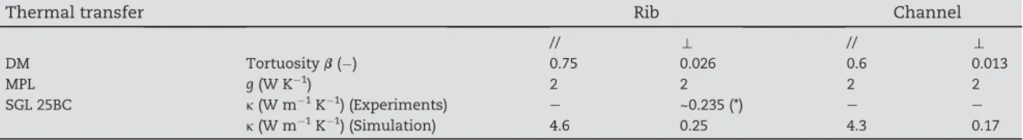
Table 3 e Coefficients used for modeling the thermal transfer; (*) Evaluation from Ref. [45]. The thermal anisotropy is evaluated by analogy with electrical anisotropylT==
lTt
¼se== set.
Thermal transfer Rib Channel
// t // t DM Tortuosity b ($) 0.75 0.026 0.6 0.013 MPL g (W K$1) 2 2 2 2 SGL 25BC k(W m$1K$1) (Experiments) e ~0.235 (*) e e k(W m$1K$1) (Simulation) 4.6 0.25 4.3 0.17
r e f e r e n c e s
[1] Yu X, Zhou B, Sobiesiak A. Water and thermal management for Ballard PEM fuel cell stack. J Power Sources 2005;147:184e95.
[2] Borup R, Meyers J, Pivovar B, Kim YS. Scientific aspects of polymer electrolyte fuel cell durability and degradation. Chem Rev 2007;107(10):3904e51.
[3] Benziger J, Nehlsen J, Blackwell D, Brennan T, Itescu J. Water flow in the gas diffusion layer of PEM fuel cells. J Membr Sci 2005;261:98e106.
[4] Dutta S, Shimpalee S, Van Zee JW. Numerical prediction of mass-exchange between cathode and anode channels in a PEM fuel cell. Int J Heat Mass Transf 2001;44:2029e42. [5] Siegel NP, Ellis MW, Nelson DJ, von Spakovsky MR. A
two-dimensional computational model of a PEMFC with liquid water transport. J Power Sources 2004;128:173e84. [6] Meng H, Wang CY. Large-scale simulation of polymer
electrolyte fuel cells by parallel computing. Chem Eng Sci 2004;59:3331e43.
[7] Rebai M, Prat M. Scale effect and two-phase flow in a thin hydrophobic porous layer. Application to water transport in gas diffusion layers of PEM fuel cells. J Power Sources 2009;192:534e43.
[8] Gostick JT, Ioannidis MA, Fowler MW, Pritzker MD. Pore network modeling of fibrous gas diffusion layers for polymer electrolyte membrane fuel cells. J Power Sources
2007;173:277e90.
[9] Pulloor Kuttanikkad S, Prat M, Pauchet J. Pore-network simulations of two-phase flow in a thin porous layer of mixed wettability: application to water transport in gas diffusion layers of proton exchange membrane fuel cells. J Power Sources 2011;196:1145e55.
[10] Pauchet J, Prat M, Schott P, Pulloor Kuttanikkad S. Performance loss of proton exchange membrane fuel cell due to hydrophobicity loss in gas diffusion layer: analysis by multiscale approach combining pore network and performance modeling. Int J Hydrogen Energy 2012;37(2):1628e41.
[11] El Hannach M, Prat M, Pauchet J. Pore network model of the cathode catalyst layer of proton exchange membrane fuel cells: analysis of water management and electrical performance. Int J Hydrogen Energy 2012;37(4):18996e9006. [12] Belgacem N, Aga€esse T, Pauchet J, Prat M. Liquid invasion
from multiple inlet sources and optimal gas access in a two-layer thin porous medium. Transp Porous Media 2016;115(3):449e72.
[13] Gostick JT. Random pore network modeling of fibrous pemfc gas diffusion media using voronoi and delaunay
tessellations. J Electrochem Soc 2013;160(8):F731e43. [14] Aga€esse T, Lamibrac A, Buechi F, Pauchet J, Prat M. Gostick? J
Power Sources 2016;331:462e74.
[15] Straubhaar B, Pauchet J, Prat M. Pore network modelling of condensation in gas diffusion layers of proton exchange membrane fuel cells. Int J Heat Mass Transf
2016;102(1):891e901.
[16] Oberholzer P, Boillat P. Local characterization of PEFCs by differential cells: systematic variations of current and asymmetric relative humidity. J Electrochem Soc 2014;161(1):F139e52.
[17] LaManna JM, Chakraborty S, Gagliardo JJ, Mench MM. Isolation of transport mechanisms in PEFCs using high resolution neutron imaging. Int J Hydrogen Energy 2014;39:3387e96.
[18] Ceballos L, Prat M. Invasion percolation with multiple injections and the water management problem in proton exchange membrane fuel cell. J Power Sources 2010;195:825e8.
[19] Straubhaar B, Pauchet J, Prat M. Water transport in gas diffusion layers of PEM fuels cells in presence of a temperature gradient. Phase change effect. Int J Hydrogen Energy 2015;40(35):11668e75.
[20] Alink R, Gerteisen D. Modeling the liquid water transport in the gas diffusion layer for polymer electrolyte membrane fuel cells using a water path network. Energies
2013;6(9):4508e30.
[21] Alink R, Gerteisen D. Coupling of a continuum fuel cell model with a discrete liquid water percolation model. Int J Hydrogen Energy 2014;39:8457e73.
[22] Qin CZ, Hassanizadeh SM, Van Oosterhout LM. Pore-network modeling of water and vapor transport in the micro porous layer and gas diffusion layer of a polymer electrolyte fuel cell. Computation 2016;4(2):21.
[23] Zenyuk IV, Medici EF, Allen JS, Weber AZ. Coupling continuum and pore-network models for polymer-electrolyte fuel cells. Int J Hydrogen Energy 2015;40:16831e45.
[24] Medici EF, Zenyuk IV, Parkinson DY, Weber AZ, Allen JS. Understanding water transport in polymer electrolyte fuel cells using coupled continuum and pore-network models. Fuel Cells 2016;16:725e33.
[25] Aghighi M, Hoeh MA, Lehnert W, Merle G, Gostick J. Simulation of a full fuel cell membrane electrode assembly using pore network modeling. J Electrochem Soc
2016;163(5):F384e92.
[26] Stauffer D. Introduction to percolation theory. 2nd ed. CRC Press; 1994.
[27] Eller J, Rose T, Marone F, Stampanoni M, Wokaun A, Bchi FN. Progress in in situ X-ray tomographic microscopy of liquid water in gas diffusion layers of PEFC. J Electrochem Soc 2011;158(8):B963e70.
[28] http://ansatte.hin.no/ra/MatLinks/carbonfiber_overview.pdf, 20-06-2015.
[29] http://zoltek.com/carbonfiber/, 20-06-2015.
[30] Incropera FP, Dewitt DP. Fundamentals of heat and mass transfer. 5th ed. 2001.
[31] Burheim OS, Pharoah JG, Lampert H, Vie PJS, Kjelstrup S. Through-plane thermal conductivity of PEMFC porous transport layers. J Fuel Cell Sci Tech 2011;8:021013. [32] Zhang J. PEM fuel cells electrocatalysts and catalyst layers.
Springer editions, ISBN 978-1-84800-935-6. [33] Erdey-Gruz T, Volmer M. Zur theorie der
wasserstoffu¨berspannung. Z Phys Chem (A) 1930;150:203e13. [34] Mann RF, Amphlett JC, Hooper MAI, Jensen HM, Peppley BA, Roberge PR. Development and application of a generalised steady-state electrochemical model for a PEM fuel cell. J Power Sources 2000;86:173e80.
[35] Mann RF, Amphlett JC, Peppley BA, Thurgood CP. Application of ButlereVolmer equations in the modelling of activation polarization for PEM fuel cells. J Power Sources 2006;161:775e81. [36] Project Chameau, Synth#ese des !etudes de mod!elisation des
performances; unpublished CEA internal report.
[37] Kordesch K, Simader G. Fuel Cells and their applications. 1996.
[38] Springer TE, Zawodzinski TA, Gottesfeld S. Polymer electrolyte fuel cell model. J Electrochem Soc 1991;138:2334e42.
[39] Wilkinson D, Willemsen JF. Invasion percolation: a new form of percolation theory. Phys A Math Gen 1983;16:3365e76. [40] Chapuis O, Prat M, Quintard M, Chane-Kane E, Guillot O,
Mayer NJ. Two-phase flow and evaporation in model fibrous media: application to the gas diffusion layer of PEM fuel cells. J Power Sources 2008;178:258e68.
[41] Freunberger SA, Reum M, Evert J, Wokau A, Bu¨chi FN. Measuring the current distribution in PEFCs with sub-millimeter resolution. J Electrochem Soc 2006;153:A2158e65. [42] Rachidi S. D!eveloppement et exploitation d'une
[unpublished Ph.D. thesis]. France: Grenoble University; 2011.
[43] LaManna JM, Kandlikar SG. Determination of effective water vapor diffusion coefficient in pemfc gas diffusion layers. Int J Hydrogen Energy 2011;36:5021e9.
[44] http://fuelcellmarkets.com/content/images/articles/GDL_24_ 25_Series_Gas_Diffusion_Layer.pdf, 20-06-2015.
[45] Thomas A, Maranzana G, Didierjean S, Dillet J, Lottin O. Thermal and water transfer in PEMFCs: investigating the role of the microporous layer. Int J Hydrogen Energy 2014;39:2649e58.