Bayesian M/EEG source localization with possible joint skull conductivity estimation

DOCTORAT DE L'UNIVERSITÉ DE TOULOUSE

Délivré par :

Institut National Polytechnique de Toulouse (INP Toulouse)

Discipline ou spécialité :

Image, Information et Hypermédia

Présentée et soutenue par :

M. FACUNDO HERNAN COSTA

le jeudi 2 mars 2017

Titre :

Unité de recherche :

Ecole doctorale :

Bayesian M/EEG Source Localization with possible Joint Skull Conductivity

Estimation

Mathématiques, Informatique, Télécommunications de Toulouse (MITT)

Institut de Recherche en Informatique de Toulouse (I.R.I.T.)

Directeur(s) de Thèse :

M. JEAN YVES TOURNERET M. HADJ BATATIA

Rapporteurs :

M. DAVID BRIE, UNIVERSITÉ LORRAINE M. LAURENT ALBERA, UNIVERSITE RENNES 1

Membre(s) du jury :

1 M. ANDRE FERRARI, UNIVERSITE DE NICE SOPHIA ANTIPOLIS, Président

2 M. HADJ BATATIA, INP TOULOUSE, Membre

2 M. JEAN YVES TOURNERET, INP TOULOUSE, Membre

A

BSTRACT

M/EEG mechanisms allow determining changes in the brain activity, which is useful in diagnosing brain disorders such as epilepsy. They consist of measur-ing the electric potential at the scalp and the magnetic field around the head. The measurements are related to the underlying brain activity by a linear model that depends on the lead-field matrix. Localizing the sources, or dipoles, of M/EEG measurements consists of inverting this linear model. However, the non-uniqueness of the solution (due to the fundamental law of physics) and the low number of dipoles make the inverse problem ill-posed. Solving such problem requires some sort of regularization to reduce the search space. The literature abounds of methods and techniques to solve this problem, especially with variational approaches.

This thesis develops Bayesian methods to solve ill-posed inverse problems, with application to M/EEG. The main idea underlying this work is to constrain sources to be sparse. This hypothesis is valid in many applications such as cer-tain types of epilepsy. We develop different hierarchical models to account for the sparsity of the sources.

Theoretically, enforcing sparsity is equivalent to minimizing a cost function penalized by an`0pseudo norm of the solution. However, since the`0 regular-ization leads to NP-hard problems, the`1approximation is usually preferred. Our first contribution consists of combining the two norms in a Bayesian frame-work, using a Bernoulli-Laplace prior. A Markov chain Monte Carlo (MCMC) al-gorithm is used to estimate the parameters of the model jointly with the source location and intensity. Comparing the results, in several scenarios, with those obtained with sLoreta and the weighted`1norm regularization shows interest-ing performance, at the price of a higher computational complexity.

Our Bernoulli-Laplace model solves the source localization problem at one instant of time. However, it is biophysically well-known that the brain activity follows spatiotemporal patterns. Exploiting the temporal dimension is

there-fore interesting to further constrain the problem. Our second contribution consists of formulating a structured sparsity model to exploit this biophysical phenomenon. Precisely, a multivariate Bernoulli-Laplacian distribution is pro-posed as an a priori distribution for the dipole locations. A latent variable is in-troduced to handle the resulting complex posterior and an original Metropolis-Hastings sampling algorithm is developed. The results show that the proposed sampling technique improves significantly the convergence. A comparative analysis of the results is performed between the proposed model, an`21mixed norm regularization and the Multiple Sparse Priors (MSP) algorithm. Various experiments are conducted with synthetic and real data. Results show that our model has several advantages including a better recovery of the dipole loca-tions.

The previous two algorithms consider a fully known lead-field matrix. How-ever, this is seldom the case in practical applications. Instead, this matrix is the result of approximation methods that lead to significant uncertainties. Our third contribution consists of handling the uncertainty of the lead-field ma-trix. The proposed method consists in expressing this matrix as a function of the skull conductivity using a polynomial matrix interpolation technique. The conductivity is considered as the main source of uncertainty of the lead-field matrix. Our multivariate Bernoulli-Laplacian model is then extended to esti-mate the skull conductivity jointly with the brain activity. The resulting model is compared to other methods including the techniques of Vallaghé et al and Guttierez et al. Our method provides results of better quality without requiring knowledge of the active dipole positions and is not limited to a single dipole activation.

R

ÉSUMÉ

Les techniques M/EEG permettent de déterminer les changements de l’activité du cerveau, utiles au diagnostic de pathologies cérébrales, telle que l’épilepsie. Ces techniques consistent à mesurer les potentiels électriques sur le scalp et le champ magnétique autour de la tête. Ces mesures sont reliées à l’activité élec-trique du cerveau par un modèle linéaire dépendant d’une matrice de mélange liée à un modèle physique.

La localisation des sources, ou dipôles, des mesures M/EEG consiste à in-verser le modèle physique. Cependant, la non-unicité de la solution (due à la loi fondamentale de physique) et le faible nombre de dipôles rendent le prob-lème inverse mal-posé. Sa résolution requiert une forme de régularisation pour restreindre l’espace de recherche. La littérature compte un nombre important de travaux traitant de ce problème, notamment avec des approches variation-nelles.

Cette thèse développe des méthodes Bayésiennes pour résoudre des prob-lèmes inverses, avec application au traitement des signaux M/EEG. L’idée prin-cipale sous-jacente à ce travail est de contraindre les sources à être parcimonieuses. Cette hypothèse est valide dans plusieurs applications, en particulier pour cer-taines formes d’épilepsie. Nous développons différents modèles Bayésiens hiérar-chiques pour considérer la parcimonie des sources.

En théorie, contraindre la parcimonie des sources équivaut à minimiser une fonction de coût pénalisée par la norme`0de leurs positions. Cependant, la régularisation`0générant des problèmes NP-complets, l’approximation de cette pseudo-norme par la norme`1est souvent adoptée. Notre première con-tribution consiste à combiner les deux normes dans un cadre Bayésien, à l’aide d’une loi a priori Bernoulli-Laplace. Un algorithme Monte Carlo par chaîne de Markov est utilisé pour estimer conjointement les paramètres du modèle et les positions et intensités des sources. La comparaison des résultats, selon plusieurs scénarii, avec ceux obtenus par sLoreta et la régularisation par la

norme`1montre des performances intéressantes, mais au détriment d’un coût de calcul relativement élevé.

Notre modèle Bernoulli-Laplace résout le problème de localisation des sources pour un instant donné. Cependant, il est admis que l’activité cérébrale a une certaine structure spatio-temporelle. L’exploitation de la dimension temporelle est par conséquent intéressante pour contraindre d’avantage le problème. Notre seconde contribution consiste à formuler un modèle de parcimonie structurée pour exploiter ce phénomène biophysique. Précisément, une distribution Bernoulli-Laplacienne multivariée est proposée comme loi a priori pour les dipôles. Une variable latente est introduite pour traiter la loi a posteriori complexe résul-tante et un algorithme d’échantillonnage original de type Metropolis-Hastings est développé. Les résultats montrent que la technique d’échantillonnage pro-posée améliore significativement la convergence de la méthode MCMC. Une analyse comparative des résultats a été réalisée entre la méthode proposée, une régularisation par la norme mixte`21, et l’algorithme MSP (Multiple Sparse Priors). De nombreuses expérimentations ont été faites avec des données syn-thétiques et des données réelles. Les résultats montrent que notre méthode a plusieurs avantages, notamment une meilleure localisation des dipôles.

Nos deux précédents algorithmes considèrent que le modèle physique est entièrement connu. Cependant, cela est rarement le cas dans les applications pratiques. Au contraire, la matrice du modèle physique est le résultat de méth-odes d’approximation qui conduisent à des incertitudes significatives. Notre troisième contribution consiste à considérer l’incertitude du modèle physique dans le problème de localisation de sources. La méthode proposée consiste à exprimer la matrice de mélange du modèle comme une fonction de la conduc-tivité du crâne, en utilisant une technique d’interpolation polynomiale. La con-ductivité est considérée comme la source principale de l’incertitude du modèle physique et elle est estimée à partir des données. La distribution Bernoulli-Laplacienne multivariée est étendue pour estimer la conductivité conjointe-ment avec l’activité cérébrale. Le modèle résultant est comparé à d’autres méth-odes en particulier les techniques de Vallaghé et al. et Guttierez et al. Notre méthode fournit des résultats de meilleure qualité sans connaissance préalable de la position des dipôles actifs, et n’est pas limitée à un dipôle unique.

C

ONTENTS

1 Introduction 16

1.1 Motivation . . . 16

1.2 Organization of the manuscript . . . 17

1.3 Publications . . . 18 2 Medical Context 20 2.1 M/EEG measurements . . . 20 2.2 Preprocessing . . . 21 2.3 Source Localization . . . 22 2.3.1 Leadfield matrix . . . 22

2.3.2 Methods with known leadfield matrix . . . 23

2.3.3 Methods with unknown leadfield matrix . . . 25

2.3.4 M/EEG Source Localization . . . 26

2.4 Conclusion . . . 26

3 Bayesian Sparse M/EEG Source Localization 28 3.1 Introduction . . . 29

3.2 Proposed Bayesian model . . . 29

3.2.1 Likelihood . . . 29 3.2.2 Prior distributions . . . 30 3.2.3 Hyperparameter priors . . . 31 3.2.4 Posterior distribution . . . 32 3.3 Gibbs sampler . . . 32 3.3.1 Conditional distributions . . . 33 3.3.2 Parameter estimators . . . 34 3.4 Experimental results . . . 35 3.4.1 Synthetic data . . . 35 3.4.2 Real data . . . 45

3.4.3 Computational cost . . . 52

3.5 Conclusion . . . 53

4 Bayesian M/EEG Source localization using structured sparsity 55 4.1 Introduction . . . 56

4.2 Proposed Bayesian model . . . 56

4.2.1 Likelihood . . . 57

4.2.2 Prior distributions . . . 57

4.2.3 Hyperparameter priors . . . 59

4.2.4 Posterior distribution . . . 61

4.3 Partially collapsed Gibbs sampler . . . 61

4.3.1 Conditional distributions . . . 61

4.4 Improving convergence . . . 64

4.4.1 Local maxima . . . 64

4.4.2 Multiple dipole shift proposals . . . 64

4.4.3 Inter-chain proposals . . . 68 4.4.4 Parameter estimators . . . 69 4.5 Experimental results . . . 71 4.5.1 Synthetic data . . . 71 4.5.2 Real data . . . 81 4.5.3 Computational cost . . . 88 4.6 Conclusion . . . 88

5 Joint M/EEG source localization and Skull Conductivity Estimation 90 5.1 Introduction . . . 91

5.2 Proposed Bayesian model . . . 91

5.2.1 Matrix normalization . . . 92

5.2.2 Likelihood . . . 92

5.2.3 Prior and hyperprior distributions . . . 92

5.2.4 Posterior distribution . . . 94

5.3 Partially collapsed Gibbs sampler . . . 94

5.3.1 Conditional distributions . . . 95

5.4 Leadfield matrix Approximation . . . 96

5.4.1 Dependency analysis . . . 96

5.4.2 Polynomial approximation . . . 97

5.4.3 Skull conductivity sampling . . . 98

5.5 Improving the convergence of the Gibbs sampler . . . 99

5.5.2 Inter-chain proposals . . . 100 5.6 Experimental Results . . . 101 5.6.1 Synthetic data . . . 101 5.6.2 Real data . . . 117 5.6.3 Computational cost . . . 121 5.7 Conclusion . . . 123

6 Conclusion and Future Work 124 6.1 Conclusions . . . 124

6.2 Future work . . . 126

A Conditional probability distributions derivations 129 A.1 Introduction . . . 129

A.2 Structured sparsity model . . . 129

A.2.1 Posterior distribution . . . 129

A.2.2 Conditional distributions . . . 130

A.3 Skull conductivity joint estimation model . . . 135

A.3.1 Posterior distribution . . . 135

A.3.2 Conditional distributions . . . 135

A

CRONYMS

BEM Boundary Element Method

ECG Electrocardiography

EEG Electroencephalography

EIT Electrical Impedance Tomography

FDM Finite Difference Method

FEM Finite Element Method

FINES First priNcipal vEctorS

FMRI Functional MRI

LORETA LOw-Resolution Electromagnetic Tomography Algorithm

MCMC Markov chain Monte Carlo

MEG Magnetoencephalography

M/EEG Magnetoelectroencephalography

MH Metropolis-Hastings

MMSE Minimum MSE

MNE Minimum Norm Estimates

MRI Magnetic Resonance Imaging

MSE Mean Square Error

MSP Multiple Sparse Priors

MUSIC MUltiple SIgnal Classification

PDF Probability Density Function

PSRF Potential Scale Reduction Factor

R-MUSIC Recursive MUSIC

RAP-MUSIC Recursively APplied MUSIC

SLORETA Standardized LORETA

SNR Signal to Noise Ratio

P

ROBABILITY DISTRIBUTIONS

Be(α,β) Beta distribution with shape parameterα and rate parameter β G (α,β) Gamma distribution with shape parameterα and rate parameter β G I G (a,b,p) Generalized Inverse Gaussian distribution with parameters a, b and p I G (α,β) Inverse gamma distribution with shape parameterα and rate parameter β N (µ,Σ) Normal distribution with meanµ and covariance Σ

N+(µ,Σ) Normal distribution with meanµ and covariance Σ truncated on R+ N−(µ,Σ) Normal distribution with meanµ and covariance Σ truncated on R− U (a,b) Uniform distribution with lower limit a and upper limit b

L

IST OF

F

IGURES

2.1 Typical sensors setups for EEG and MEG measurements. . . 21

2.2 Shell and realistic brain model representations. . . 23

3.1 Directed acyclic graph of the hierarchy used for the Bayesian model.

. . . 31

3.2 Simulation results for single dipole experiments. The horizon-tal axis indicates the activation number. The error bars show the standard deviation over 12 Monte Carlo runs. . . 38

3.3 Brain activity for one single dipole experiment (activation #5). . . 39

3.4 Histogram of samples generated by the MCMC method for one of the single dipole simulations. The estimated mean values and ground truth are indicated in the figures. . . 40

3.5 Brain activity for a multiple distant dipole experiment (activation # 2 that has two active dipoles). . . 42

3.6 Brain activity for a multiple distant dipole experiment (activation # 3 that has three active dipoles). . . 43

3.7 Transportation cost for multiple distant dipoles experiments, the horizontal axis indicates the activation number (1 and 2: two ac-tive dipoles, 3 and 4: three acac-tive dipoles). The error bars show the standard deviation over 12 Monte Carlo runs. . . 44

3.8 Transportation cost for multiple close dipoles experiments. The horizontal axis indicates the activation number (1 and 2: 50mm separation, 3 and 4: 30mm separation, 5 and 6: 10mm separa-tion). The error bars show the standard deviation over 12 Monte Carlo runs. . . 45

3.9 Brain activity for multiple close dipoles (activation # 4 that has a 30mm separation between dipoles). . . 46

3.10 Brain activity for multiple close dipoles (activation # 6 that has a

10mm separation between dipoles). . . 47

3.11 M/EEG measurements for the real data application. . . 49

3.12 Brain activity for the auditory evoked responses from 80ms to 126ms. 50 3.13 Brain activity for the faced evoked responses for 160ms. . . 51

4.1 Directed acyclic graph for the proposed Bayesian model. . . 60

4.2 Example of posterior distribution ofzwith local maxima . . . 64

4.3 Illustration of the effectiveness of the multiple dipole shift pro-posals. . . 65

4.4 Efficiency of the inter-chain proposal. . . 70

4.5 Estimated waveforms for three dipoles with SNR = 30dB.. . . 72

4.6 Estimated activity for three dipoles and SNR = 30dB. . . 73

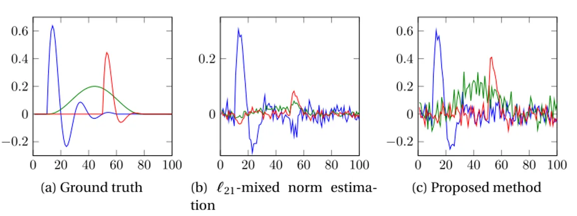
4.7 Estimated waveforms for three dipoles with SNR = -3dB. . . 74

4.8 Estimated activity for three dipoles and SNR = -3dB. . . 75

4.9 Estimated boundariesµ ± 2σ for the three dipole simulation with SNR = -3dB. . . 76

4.10 Three dipoles with SNR = -3dB: histograms of the hyperparame-ters. The actual values ofω and σ2_nare marked with a red vertical line. . . 76

4.11 Three dipoles with SNR = -3dB: PSRFs of sampled variables.. . . . 77

4.12 Estimated activity for five dipoles and SNR = 30dB. . . 78

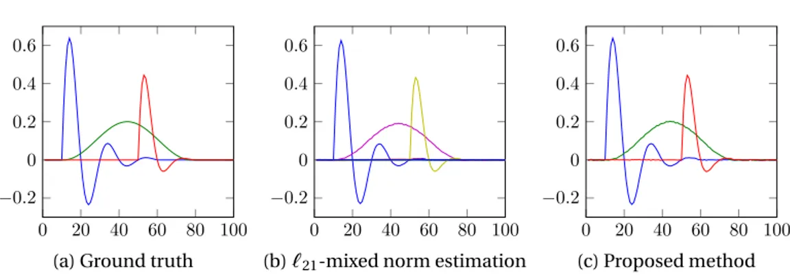
4.13 Estimated waveforms for five dipoles with SNR = 30dB. Green rep-resents the ground truth, blue the`21mixed norm estimation and red the proposed method. . . 79

4.14 Performance measures for multiple dipoles. . . 80

4.15 Measurements and estimated waveforms for the auditory evoked responses. . . 81

4.16 Estimated activity for the auditory evoked responses.. . . 82

4.17 Estimated waveforms mean and boundariesµ ± 2σ for the audi-tory evoked responses. . . 83

4.18 Hyperparameter histograms for the auditory evoked responses. . 84

4.19 PSRFs of sampled variables for the auditory evoked responses .. . 85

4.20 Measurements and estimated waveforms for the facial evoked re-sponses. . . 86

4.21 Estimated activity for the facial evoked responses. . . 87

5.2 Variations of the matrix elements with respect toρ. . . . 97

5.3 RMSE ofρ VS L (K = 100). . . . 102

5.4 RMSE ofρ VS K (L = 7). . . . 103

5.5 Estimated marginal posterior distributions of the different model parameters for the proposed model (ρ estimated) for simulation #1 (single dipole) . . . 105

5.6 Estimated marginal posterior distributions of the default-ρ model (ρ = ρfixis not estimated) for simulation #1 (single dipole). . . 106

5.7 Recovered waveforms for the single dipole simulation #1. . . 106

5.8 Estimated activity for single dipole simulation #2. . . 108

5.9 Estimated waveforms for simulation #2 (single dipole) . . . 109

5.10 PSRFs for the proposed method versus the number of iterations for simulation #1 (single dipole). . . 109

5.11 Estimated conductivity for the multiple dipole depths experiments (SNR = 30dB). . . 111

5.12 Estimated conductivity for the multiple dipole depths experiments (SNR = 20dB). . . 112

5.13 Estimated conductivity for the multiple dipole depths experiments (SNR = 15dB). . . 113

5.14 Estimated conductivity for the multiple dipole depths experiments (SNR = 10dB). . . 114

5.15 Performance measures for the estimation of multiple dipoles as a function of C . . . . 115

5.16 Estimated activity for the auditory evoked responses.. . . 118

5.17 Estimated waveforms for the auditory evoked responses. . . 119

5.18 Estimated waveforms mean and boundariesµ ± 2σ for the audi-tory evoked responses using the proposed model. . . 119

5.19 Estimated parameter distributions for the auditory evoked responses.120 5.20 PSRFs of the sampled variables for the auditory evoked responses along iterations. . . 122

L

IST OF

T

ABLES

3.1 Computation costs of the different algorithms (in seconds). . . 53

4.1 Three dipoles with SNR = -3dB: modes explored after convergence. Positions 1, 2 and 3 correspond to the non-zero elements of the ground truth. . . 72

5.1 Prior distributions f (zi|ω), f (τ2_i|a), f ( ¯xi|zi,τ2_i,σ2n), f (σ2n), f (a)

and f (ω). . . . 93

5.2 Conditional distributions f (τ2_i|xi,σ2n, a, zi), f (zi|Y,X−i,σ2n,τ2i,ω,ρ),

f (xi|zi,Y,X−i,σ2n,τ2i,ρ), f (a|τ2), f (σ2n|Y,X,τ2,z,ρ) and f (ω|z). 95

5.3 Estimation errors for the different parameters (Simulation #1) . . 104

L

IST OF

A

LGORITHMS

3.1 Gibbs sampler.. . . 32

4.1 Partially Collapsed Gibbs sampler. . . 62

4.2 Multiple dipole shift proposal. . . 67

4.3 Inter-chain proposals. . . 69

5.1 Partially Collapsed Gibbs sampler. . . 95

5.2 Multiple dipole shift proposal. . . 99

C

HAPTER

1

I

NTRODUCTION

Contents

1.1 Motivation . . . . 16

1.2 Organization of the manuscript . . . . 17

1.3 Publications . . . . 18

1.1

M

OTIVATION

Recent World Health Organization data suggest that neurological disorders, in-cluding epilepsy, are one of the most important contributors to the global bur-den of human suffering [1]. M/EEG measurement is one of the main tools used by specialists to examine epilepsy patients. Other uses of M/EEG include eval-uation of encephalopaties and focal brain lesions [1].

M/EEG is a powerful non-invasive technique that measures the electric po-tentials at the scalp and the magnetic fields around the head. These measure-ments depend upon 1) the underlying brain activity and 2) the geometric com-position of the head. The recovery of the brain activity from the measurements is an ill-posed inverse problem. Thus, a regularization is needed to have a nar-row the search space. This regularization should typically be chosen to con-strain the solution to have some realistic properties.

In this thesis we propose new Bayesian approaches to solve the M/EEG source localization problem. Our work is specifically focused on cases where the brain activity is spatially concentrated, such as in certain forms of epilepsy.

The main idea underlying the thesis is to develop Baysian sparse models for the sources. More precisely, three contributions are presented:

(i) Developing a hierarchical Bayesian model that solves the source localiza-tion problem for one instant of time by promoting sparsity using Bernoulli-Laplacian priors [2].

(ii) Investigating a Bayesian structured sparsity model to exploit the tempo-ral dimension of the M/EEG measurements [3,4].

(iii) Developing Metropolis-Hasting sampling scheme that improves signifi-cantly the speed of the convergence of our MCMC algorithm [5].

(iv) Expanding the model to estimate the skull conductivity jointly with the brain activity [6].

1.2

O

RGANIZATION OF THE MANUSCRIPT

Chapter 2: Medical Context

This chapter provides an introduction to M/EEG, the link between elec-tric brain activity and the M/EEG measurements and the preprocessing techniques that are typically used to clean the signal. We then focus on how these measurements are used in solving the source localization prob-lem and describe state-of-the-art algorithms that have been developed in the literature with their advantages and disadvantages.

Chapter 3: Bayesian Sparse M/EEG Source Localization

In this chapter, we present a hierarchical Bayesian model aimed to solv-ing the source localization problem by promotsolv-ing sparsity. Ideally the`0 pseudo norm regularization should be used to regularize this problem. However, due to its intractability, the`0pseudo norm is usually replaced by the`1norm. Our model proposes to combine both of them, result-ing in`0and`1regularizations in a Bayesian framework to pursue sparse solutions.

Chapter 4: Structured Sparsity Bayesian M/EEG Source Localization

In this chapter, we improve the model of Chapter 3 to take advantage of the temporal structure of the M/EEG measurements. This is done by changing the prior associated with the brain activity and computing a

Bayesian approximation of the M/EEG source localization problem us-ing an `20 pseudo mixed norm regularization. This type of norm pro-motes sparsity among different dipoles (via the`0portion of the norm) and groups all the time samples of the same dipole together, forcing them all to be either jointly active or inactive (with the`2norm portion).

Chapter 5: Myopic Skull Conductivity Estimation

When working with real data, certain parameters needed to calculate the leadfield matrix are not always known. Out of these, the skull conductiv-ity stands out since it varies significantly among subjects and can affect the results of the brain activity reconstruction significantly. In this chap-ter we generalize the model to estimate the skull conductivity jointly with the brain activity. This is done by approximating the dependency of the operator with respect to the skull conductivity with a polynomial matrix.

Chapter 6: Conclusion and Future Work

This chapter presents some conclusions based on our work and some ideas that should be pursued in the near future related to it.

Appendix A: Conditional probability distributions derivations

This appendix shows the algebraic derivations of the conditional prob-ability distributions associated with the Bayesian models introduced in Chapters 4 and 5.

1.3

P

UBLICATIONS

Journal papers

(i) F. Costa, H. Batatia, L. Chaari, and J.-Y. Tourneret, “Sparse EEG Source Localization using Bernoulli Laplacian Priors,” IEEE Trans. Biomed. Eng., vol. 62, no. 12, pp. 2888–2898, 2015.

(ii) F. Costa, H. Batatia, T. Oberlin, C. D’Giano, and J.-Y. Tourneret, “Bayesian EEG source localization using a structured sparsity prior,” NeuroImage, vol. 144, pp. 142–152, jan. 2017.

(iii) F. Costa, H. Batatia, T. Oberlin, and J.-Y. Tourneret, “Skull Conductivity Estimation for EEG Reconstruction,” IEEE Signal Process. Lett., to be pub-lished.

Conference papers

(i) F. Costa, H. Batatia, T. Oberlin, and J.-Y. Tourneret, “EEG source localiza-tion based on a structured sparsity prior and a partially collapsed gibbs sampler,” in Proc. of International Workshop on Computational Advances

in Multi-Sensor Adaptive Processing (CAMSAP’15), Cancun, Mexico, 2015.

(ii) F. Costa, H. Batatia, T. Oberlin, and J.-Y. Tourneret, “A partially collapsed gibbs sampler with accelerated convergence for EEG source localization,” in Proc. of IEEE Workshop on Stat. Sig. Proc. (SSP’16), Palma de Mallorca, Spain, 2016.

(iii) Y. Mejía, F. Costa, H. Argüello, J.-Y. Tourneret and H. Batatia “Bayesian re-construction of hyperspectral images by using compressed sensing mea-surements and a local structured prior,” in Proc. IEEE Int. Conf. Acoust.,

C

HAPTER

2

M

EDICAL

C

ONTEXT

Contents

2.3.2 Methods with known leadfield matrix . . . 23

2.3.3 Methods with unknown leadfield matrix . . . 25

2.3.4 M/EEG Source Localization . . . 26

2.4 Conclusion . . . . 26

2.1

M/EEG

MEASUREMENTS

In the past decades, several non-invasive techniques for measuring brain ac-tivity have been developed. Among them, M/EEG has the noticeable advan-tage of being able to track brain activity with a temporal resolution in the order of the milliseconds. This makes it an invaluable tool in a variety of medical applications including the diagnosis of epilepsy, sleeping disorders, coma, en-cephalopathies, and brain death [7,8].

M/EEG is a combination between EEG and MEG. EEG consists in record-ing the electrical voltage, typically in the order of µV, measured by electrodes placed over the scalp (shown in Fig. 2.1a). On the other side, MEG consists

(a) EEG electrodes. (b) MEG magnetometers.

Figure 2.1: Typical sensors setups for EEG and MEG measurements.

in recording the magnetic fields using very sensitive magnetometers placed around the head (shown in Fig. 2.1b). Both the electrical voltage measured by EEG and the magnetic fields measured by MEG are generated by the brain activity of the subject that can be modeled by currents [9].

2.2

P

REPROCESSING

The measured M/EEG signal is typically highpass filtered at approximately 0.5 Hz to remove very low frequency interference (such as breathing). A lowpass filter is also applied to eliminate measurement noise higher than 50 – 70 Hz approximately. Unfortunately, the measured M/EEG signal can also be con-taminated by artifacts that are not related with the brain activity of interest and cannot be filtered out as easily [10]. The most important artifact source is the power-line interference at 50 Hz (or 60 Hz). The easiest way to deal with this in-terference is to just discard measurements in which the artifact noise is higher than a certain threshold. There are also other techniques to deal with power-line noise such as physical solutions [10,11] and adaptive noise cancelling tech-niques [12,13].

In addition to power-line noise, M/EEG measurements can also be con-taminated by other signals that originate from the patient but are not related to brain activity, such as eye movement, muscle noise and heart signal. To compensate for eye movement artifacts an additional EEG electrode is

typi-cally placed in the nose in order to obtain measurements that are used to iden-tify eye movement artifacts [14]. ECG artifacts are produced by electrical heart activity. Due to its high amplitude, this activity can be measured by placing electrodes in any non-cephalic part of the body. Cardiac artifacts can be sup-pressed by recording an ECG of the heart activity. In addition to algorithms aimed to reduce measurement artifacts, other techniques can also be applied in the pre-processing stage to improve the source localization such as tensor-based preprocessing [15–17].

Once the M/EEG measurements have been preprocessed, they can be used to solve the source localization problem.

2.3

S

OURCE

L

OCALIZATION

The source localization problem consists in using the cleaned M/EEG measure-ments to determine the electrical activity of the subject’s brain. The relation-ship between electric brain activity and M/EEG measurements is represented by the leadfield matrix (also called head operator). The leadfield matrix de-pends on the shape and composition of the subject’s head and will be explained in what follows.

2.3.1

L

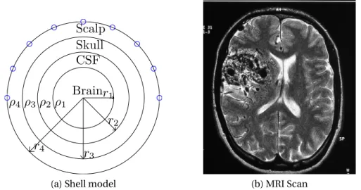
Several head models with varying precision and complexity have been used throughout the years, being mainly divided in two categories (1) the shell head models and (2) the realistic head models [18] that are displayed in Fig.2.2. The former model represents the human head using a fixed number of concentric spheres (typically 3 or 4). Each sphere corresponds to the interface between two different tissues of the human head considered to be uniform with con-stant conductivities [19]. In the three-shell head model, the skull, cerebrospinal fluid and brain tissues are considered whereas the four-shell model adds an ad-ditional outer-most sphere to model the head tissue. In order to calculate the head operator with the shell models it is necessary to set different parameters: (1) the radius of the spheres, (2) the conductivity of each tissue, (3) the amount and locations of the dipoles inside the brain and (4) the amount and locations of the electrodes in the scalp. On the other hand, the realistic head models are typically computed from the MRI of the patient in order to better represent the distribution of the different tissues inside the human head. To perform this

Brain CSF Skull Scalp ρ1 ρ2 ρ3 ρ4 r1 r2 r3 r4

(a) Shell model (b) MRI Scan

Figure 2.2: Shell and realistic brain model representations.

calculation it is possible to use several methods [18] including the boundary el-ement method (BEM) [20], the finite element method (FEM) [21] and the finite difference method (FDM) [22]. However, in order to be able to compute a head model operator from the MRI it is still necessary to set several parameters in-cluding (1) the conductivity of each tissue, (2) the amount and locations of the dipoles inside the brain and (3) the amount and locations of the electrodes in the scalp.

To ensure the quality of the activity estimation, the electrode positions and tissue conductivities should be set as close as possible to their real values. Most of the techniques developed for M/EEG source localization assume that these parameters are known in advance whereas a few consider that there can also be uncertainty in some of them. In the following we will first consider the case that assumes that the operator parameters are perfectly known in advance.

2.3.2

M

The methods that have been developed to solve the M/EEG source localization problem can be classified in two groups: (i) the dipole-fitting models that rep-resent the brain activity as a small number of dipoles with unknown positions; and (ii) the distributed-source models that represent it as a large number of dipoles at fixed positions.

The dipole-fitting models [23,24] assume that the brain activity is concen-trated in a small-number of point-like sources and estimate the location, am-plitude and orientation of a few dipoles to explain the measured data. A par-ticularity of these models is that they lead to solutions that can vary extremely with the initial guess about the number of dipoles, their locations and their ori-entations because of the existence of many local minima in the optimized cost function [25]. To solve this problem, the MUSIC algorithm [26] and its vari-ants R-MUSIC [27], RAP-MUSIC [28] and FINES [29] were developed. Another recent dipole-fitting model whose parameters are estimated using sequential Monte Carlo [30] formulates the M/EEG source localization as a semi-linear problem due to the measurements having a linear dependency with respect to the dipole amplitudes and a non-linear one with respect to the positions. If few and clustered sources are present in the underlying brain activity, the dipole-fitting algorithms generally yield good results [31, 32]. However, the perfor-mance of these algorithms can be altered in the case of multiple spatially ex-tended sources [25]. An alternative use of dipole-fitting models is as a way to find an initial iteration point for distributed-source methods [33].

On the other hand, the distributed-source methods model the brain activity as the result of a large number of discrete dipoles with fixed positions and try to estimate their amplitudes and orientations [25]. Since the amount of dipoles used in the brain model is typically much larger than the amount of measure-ments, the inverse problem is ill-posed in the sense that there is an infinite amount of brain activities that can justify the measurements [25]. A regular-ization is thus needed in order to incorporate additional information to solve this inverse problem. The kind of regularization to use should be chosen to promote realistic properties of the solution. For instance, one of the most sim-ple regularizations consists of penalizing the`2norm of the solution using the minimum norm estimation algorithm [34] or its variants based on the weighted minimum norm: Loreta [35] and sLoreta [36]. However, these methods have been shown to overestimate the size of the active area if the brain activity is focused [25], which is believed to be the case in a number of medical applica-tions. A better way to estimate focal brain activity is to promote sparsity, by applying an`0pseudo norm regularization [37]. Unfortunately, this procedure is known to be intractable in an optimization framework. As a consequence, the`0pseudo norm is usually approximated by the`1norm via convex relax-ation [38], in spite of the fact that these two approaches do not always provide the same solution [37].

in-dependently. However, to improve source localization, it is possible to make use of the temporal structure of the data by promoting structured sparsity, which is known to yield better results than standard sparsity when applied to strongly group sparse signals [39]. Structured sparsity has been shown to improve re-sults in several applications including audio restoration [40], image analysis [41] and machine learning [42]. One way of applying structured sparsity in M/EEG source localization is to use mixed-norms regularization such as the

`21mixed norm [43] (also referred to as group-lasso).

In addition to optimization techniques, several approaches have tried to model the time evolution of the dipole activity and estimate it using either Kalman filtering [44,45] or particle filters [46–48]. Several Bayesian methods have been used as well, both for dipole-fitting models [49,50] and distributed source models [51, 52]. In [51], the multiple sparse priors (MSP) approach was developed, which parcellates the brain in different pre-defined regions and promotes all the dipoles in each region to be active or inactive jointly. Doing this the brain activity is encouraged to extend over an area instead of being fo-cused in point-like sources. Conversely, we are mainly interested in estimating point-like focal source activity which has been proved to be relevant in clinical applications [53]. In order to do this, we will consider each dipole separately instead of grouping them together. Note that this approach avoids the need of choosing a criterion for brain parcellization as required in the MSP method.

2.3.3

M

In a more general case, we can consider that some of the parameters needed to calculate the operator are not perfectly known. Several authors have analyzed the influence of having errors in these parameters in the estimation of brain activity. Minor errors in the electrode positions have been shown not to affect significantly the results [54] whereas there is a much higher sensibility to varia-tions in the tissue conductivities, making their values critical [55–58]. The con-ductivities of the human head tissue, cerebrospinal fluid and brain have well known values that are accepted in the literature [55]. However, there has been some controversy regarding the conductivity of the human skull [18]. The ratio between scalp and skull conductivities was initially reported to be 80 [59] but since then other authors have published values as low as 15 [60]. The value of the human skull conductivity is also known to vary significantly across different subjects [18,61]. Because of this, it remains of interest to develop methods that estimate the skull conductivity to improve the quality of the brain activity

re-construction. This can be done using techniques such as electrical impedance tomography (EIT) [61], using intracranial electrodes [62] or measuring it di-rectly during surgery [60]. However it is also possible to estimate it directly from the M/EEG measurements.

Several methods have been proposed to estimate the conductivity of the skull and the brain activity jointly, albeit requiring very restrictive conditions to yield good results. For instance, some methods require having a very good a-priori knowledge about the active dipole positions [63, 64], others assume there is only one dipole active [65] and others limit the estimation of the skull conductivity to a few discrete values [66,67].

2.3.4

M/EEG S

L

In the most general case, M/EEG source localization can be formulated as an inverse problem that consists in estimating the brain activity of a patient from M/EEG measurements taken from M sensors during T time samples. In a dis-tributed source model, the brain activity is represented by a finite number of dipoles located at fixed positions in the brain cortex. The M/EEG measurement matrixY ∈ RM ×T can be written

Y =H(ρ)X+E [2.1]

whereX∈ RN ×T contains the dipole amplitudes,H(ρ) ∈ RM ×N represents the head operator (usually called “leadfield matrix”) that depends on the skull con-ductivityρ andEis the measurement noise.

If the value ofρ is known in advance then we have the common M/EEG source localization problem, which consists in estimating the matrixX from the known operatorH(ρ) and the measurementsY. This problem will be con-sidered in Chapters3and4. If the skull conductivityρ is not known in advance then it can be estimated jointly withX, resulting in a myope inverse problem considered in Chapter5.

2.4

C

ONCLUSION

This chapter presented a brief illustration of the M/EEG principles and the dif-ferent information that can be extracted from M/EEG measurements using sig-nal processing techniques. Among them, the source localization problem was analyzed in more detail, summarizing some state-of-the-art algorithms that are

currently being used to tackle the problem. In Chapter3we will introduce a distributed-source method that combines`0and`1regularizations to promote sparsity. This results in a model that solves the inverse problem considering each time sample independently. The initial model is later improved in Chap-ter4to promote structured sparsity using an`20mixed norm regularization in Chapter4. This model shows improved results since it takes advantage of the temporal structure of the M/EEG measurements. Finally, uncertainty in the leadfield matrix is considered. Precisely, this matrix is expressed as a function of the skull conductivityρ, which is the most important source of uncertainty. The structured sparsity model is extended in Chapter5to estimate jointly the brain activity and the skull conductivity.

C

HAPTER

3

B

AYESIAN

S

PARSE

M/EEG S

OURCE

L

OCALIZATION

Contents

3.1 Introduction . . . . 29

3.2 Proposed Bayesian model . . . . 29

3.2.1 Likelihood . . . 29 3.2.2 Prior distributions . . . 30 3.2.3 Hyperparameter priors . . . 31 3.2.4 Posterior distribution . . . 32 3.3 Gibbs sampler . . . . 32 3.3.1 Conditional distributions . . . 33 3.3.2 Parameter estimators . . . 34 3.4 Experimental results . . . . 35 3.4.1 Synthetic data . . . 35 3.4.2 Real data . . . 45 3.4.3 Computational cost . . . 52 3.5 Conclusion . . . . 53

3.1

I

NTRODUCTION

When using a distributed-source model to solve the M/EEG source localization problem, it is necessary to apply a regularization in order to have a unique so-lution. In certain medical conditions, such as certain types of epilepsy or focal lesions, brain activity is believed to be focalized in a small brain region [8], so it makes sense to choose a regularization that promotes sparsity. This should be done by applying an`0pseudo norm regularization [37]. However, due to its intractability, it is typically approximated to an`1norm despite the fact that the results of both regularizations is not always the same [37]. We propose to com-bine both`0and`1regularizations in a Bayesian framework to pursue sparse solutions.

3.2

P

ROPOSED

B

AYESIAN MODEL

This chapter is devoted to the presentation of a new Bayesian model for M/EEG source localization. The model is described in Section3.2. Section3.3studies a hybrid Gibbs sampler that will be used to generate samples asymptotically distributed according to the posterior of the model introduced in Section3.2. Simulation results obtained with synthetic and real M/EEG data are presented in Section3.4.

3.2.1

L

It is very classical in M/EEG analysis to consider an additive white Gaussian noise whose variance will be denoted asσ2_n [25]. When this assumption does not hold, it is always possible to estimate the noise covariance matrix from the data and to whiten the data before applying the algorithm [68]. The Gaussian noise assumption for the noise samples leads to the following probability den-sity function (pdf ) f (Y|X,σ2_n) = T Y t =1 N ³yt ¯ ¯ ¯Hx t_,σ2 nIM ´ [3.1] where Y ∈ RM ×T contains the M/EEG measurements, X ∈ RN ×T the dipole amplitudes andH∈ RM ×N represents the head operator (usually called “lead-field matrix”). mt is the t th column of matrixM and IM is the identity matrix

3.2.2

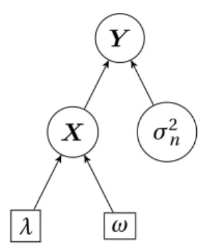
P

The unknown parameter vector associated with the likelihood [3.1] isθ = {X,σ2_n}. In order to perform Bayesian inference, we assign priors to these parameters as follows.

3.2.2.1 PRIOR FOR THE DIPOLE AMPLITUDES

As stated in Section 3.1, we want to build a regularization combining an `0 pseudo norm with an`1norm of the M/EEG source localization solution. It can be easily shown that using a Laplace prior is the Bayesian equivalent of an

`1norm regularization whereas a Bernoulli prior can be associated with the`0 pseudo-norm. As a consequence, we propose to use a Bernoulli-Laplace prior. The combination of the two norms allows the non zero elements to be localized (via the Bernoulli part of the prior) and their amplitudes to be estimated (with the Laplace distribution). Note that the Laplace distribution is able to estimate both small and high amplitudes due to its large value around zero and its fat tails. The corresponding prior for the i j th element ofXis

f (xi j|ω, λ) = (1 − ω)δ(xi j) + ω 2λexp µ −|xi j| λ ¶ [3.2] whereδ(.) is the Dirac delta function, λ is the parameter of the Laplace distri-bution, andω the weight balancing the effects of the Dirac delta function and the Laplace distribution. Assuming the random variables xi j are a priori

inde-pendent, the prior distribution ofXcan be written

f (X|ω, λ) = T Y j =1 N Y i =1 f (xi j|ω, λ). [3.3]

3.2.2.2 PRIOR FOR THE NOISE VARIANCE

A non-informative Jeffrey’s prior is assigned to the noise variance

f (σ2_{n) ∝} 1 σ2

n

1_R+(σ2_n) [3.4]

where 1_R+(x) is the indicator function onR+. This prior is a very classical choice

3.2.3

H

The hyperparameter vector associated with the previous priors isΦ = {ω,λ} as displayed in the direct acyclic graph of Fig. 3.1. We consider a hierarchical Bayesian model which allows the hyperparameters to be estimated from the data. This strategy requires to assign priors to the hyperparameters (referred to as hyperpriors) that are defined in this section.

Y X σ2_n

λ ω

Figure 3.1: Directed acyclic graph of the hierarchy used for the Bayesian model.

3.2.3.1 HYPERPRIOR FORω

An independent uniform distribution on [0,ωmax] is assigned to the weightω

ω ∼ U³0,ωmax ´

[3.5] whereωmax∈ [0, 1] is an upper bound on ω that is fixed in order to ensure a minimum level of sparsity.1

3.2.3.2 HYPERPRIOR FORλ

Using similar arguments as for the noise varianceσ2_n, a Jeffrey’s prior is assigned toλ in order to define the following non-informative prior

f (λ) ∝ 1

λ1R+(λ). [3.6]

1_{We have observed that settingω}

max< 1 (instead of ωmax= 1) yields faster convergence of

3.2.4

P

Taking into account the likelihood and priors introduced above, the joint pos-terior distribution of the model used for M/EEG source localization can be ex-pressed using the following hierarchical structure

f (θ,Φ|Y) ∝ f (Y|θ) f (θ|Φ) f (Φ) [3.7] where {θ,Φ} is the vector containing the model parameters and hyperparam-eters. Because of the complexity of this posterior distribution, the Bayesian estimators of {θ,Φ} cannot be computed with simple closed-form expressions. Section3.3studies an MCMC method that can be used to sample the joint pos-terior distribution [3.7] and build Bayesian estimators of the unknown model parameters using the generated samples.

3.3

G

IBBS SAMPLER

This section considers a Gibbs sampler [69] which generates samples itera-tively from the conditional distributions of [3.7], i.e., from f (σ2_n|Y,X), f (λ|X),

f (ω|X) and f (xi j|Y,X−i j,ω,λ,σ2n) whereM−i j denotes the matrixM whose

i j th element has been replaced by zero. The next sections explain how to

sam-ple from the conditional distributions of the unknown parameters and hyper-parameters associated with the posterior of interest [3.7]. The resulting algo-rithm is also summarized in Algoalgo-rithm3.1.

Algorithm 3.1 Gibbs sampler.

InitializeXwith the sLoreta solution

repeat Sampleσ2_naccording to f (σ2_n|X,Y). Sampleλ according to f (λ|X). Sampleω according to f (ω|X). for j = 1 to T do for i = 1 to M do

Sample xi j according to f (xi j|Y,X−i j,ω,λ,σ2n).

end for end for

3.3.1

C

3.3.1.1 CONDITIONAL DISTRIBUTION OFσ2_n

Using [3.7], it is straightforward to derive the conditional posterior distribution ofσ2_nwhich is the following inverse gamma distribution

σ2 n|X,Y ∼ I G ³ σ2 n ¯ ¯ ¯ M 2 , ||Y −HX||2 2 ´ [3.8] where ||.|| represents the euclidean norm.

3.3.1.2 CONDITIONAL DISTRIBUTION OFλ

By using f (X|ω, λ) and the prior distribution of λ, it is easy to derive the con-ditional distribution ofλ which is also an inverse gamma distribution

λ|X∼ I G ³

λ | ||X||0, ||X||1 ´

[3.9] where ||.||1is the`1norm and ||.||0the`0norm.

3.3.1.3 CONDITIONAL DISTRIBUTION OFω

Using f (X|ω, λ) and the prior of ω it can be shown that the conditional distri-bution ofω is a truncated Beta distribution defined on the interval [0,ωmax]

ω|X∼ Be[0,ωmax](1 + ||X||0, 1 + M − ||X||0). [3.10]

3.3.1.4 CONDITIONAL DISTRIBUTION OFxi j

Using the likelihood and the prior distribution ofX, the conditional distribu-tion of each signal element xi jcan be expressed as follows

f (xi j|Y,X−i j,ω,λ,σ2n, zi j) =    δ(xi j) if zi j= 0 N+(µi j ,+,σ2i) if zi j= 1 N−(µi j ,−,σ2i) if zi j= −1 [3.11]

whereN₊andN₋denote the truncated Gaussian distributions onR+andR−, respectively. The variable zi j is a discrete random variable that takes value 0

ω3,i j. More precisely, defining vi j =yj−Hx_−ij , the weights (ωl ,i j)1≤l ≤3 are defined as ωl ,i j= ul ,i j 3 P l =1 ul ,i j [3.12] where u1,i j =1 − ω u2,i j = ω 2λexp à (µ+_{i j})2 2σ2_i ! q 2πσ2_iC (µ+_{i j},σ2_i) u3,i j =ω 2λexp à (µ−_{i j})2 2σ2_i ! q 2πσ2_iC (−µ−i j,σ2i) [3.13] and σ2 i = σ2 n ||hi||2 µ+ i j=σ2i µhT ivi j σ2 n −1 λ ¶ µ− i j=σ2i µ_hT ivi j σ2 n +1 λ ¶ C (µ,σ2_{) =}1 2 · 1 + erf µ µ p 2σ2 ¶¸ . [3.14]

The truncated Gaussian distributions are sampled according to the algo-rithm specified in [70].

3.3.2

P

Using all the generated samples, the potential scale reduction factors (PSRFs) of all the model parameters and hyperparameters were calculated for each it-eration. The samples corresponding to iterations where the PSRFs were above 1.2 were discarded since they were considered to be part of the burn-in period of the sampler, as recommended by [71]. The rest were kept for calculating the estimators of the model parameters and hyperparameters following

ˆ Z , arg max ¯ Z∈{0,1,−1}N ³ #M ( ¯Z) ´ [3.15] ˆ p_, 1 #M ( ˆZ) X m∈M ( ˆZ) p(m) [3.16]

where #S denotes the cardinal of set S , M ( ¯Z) is the set of iteration numbers

m for whichZ(m)= ¯Zafter the burn-in period of the Gibbs sampler and p(m) is the m-th sample of p ∈ {X, λ, σ2_n,ω}. Thus the estimator ˆZ in [3.15] is the maximum a posteriori estimator of ˆZ whereas the estimator used for all the other sampled variables in [3.16] is the minimum mean square error (MMSE) estimator conditionally to ˆZ.

3.4

E

XPERIMENTAL RESULTS

This section reports different experiments conducted to evaluate the perfor-mance of the proposed M/EEG source localization algorithm for synthetic and real data. In these experiments, our algorithm was initialized with the sLoreta solution obtained after estimating the regularization parameter by minimizing the cross-validation error as recommended in [36]. The upper bound of the sparsity level was set to ωmax = 0.5, which is much larger than the expected value of ω. The results obtained with synthetic and real data are reported in two separate sections.

3.4.1

S

3.4.1.1 SIMULATION SCENARIO

Synthetic data with few pointwise source activations were generated using a realistic BEM head model with 19 electrodes placed according to the 10−20 in-ternational system of electrode placement. Three different kinds of activations were investigated: (i) single dipole activations, (ii) multiple distant dipole acti-vations and (iii) multiple close dipole actiacti-vations. The default subject anatomy of the Brainstorm software [72] was considered. This model corresponds to MRI measurements of a 27 year old male using the boundary element model implemented by the OpenMEEG package [73]. The default brain cortex of this subject was downsampled to generate a 1003-dipole head model. These dipoles

are distributed along the cortex surface and have an orientation normal to it, as discussed in the previous sections. The resulting head model is such that

H∈ R19×1003.

For each of the activationsX∈ R1003×1that are described in what follows, three independent white Gaussian noise realizations were added to the observed sig-nalHX, resulting in three sets of measurementsY with an SNR of 20dB. For each of these three noisy signalsY, four MCMC independent chains were run, resulting in 12 total simulations for each of the considered activationsX. The

`1and sLoreta methods were applied to the same three different sets of mea-surementsY resulting in 3 simulations for each activation.

3.4.1.2 PERFORMANCE EVALUATION

To assess the quality of the localization results, the following indicators were used

• Localization error [25]: The euclidean distance between the maximum of the estimated activity and the real source location is used to determine whether the algorithm is able to find the point of highest activity correctly or not.

• Center-mass localization error [74]: The euclidean distance between the barycenter of the estimated activity and the real source location allows us to appreciate if the activity estimated by the algorithm is centered around the correct point or if it is biased.

• Excitation extension: The spatial extension of the spatial area of the brain cortex that is estimated to be active was considered in [74]. Since the syn-thetic data only contains pointwise sources, this criterion should ideally be equal to zero.

• Transportation cost: This indicator evaluates the performance in a mul-tiple dipole situation where the activity estimates from different dipoles may overlap. It is computed as the solution of an optimal mass transport optimization problem [75] considering the known ground truth to be the initial mass distribution and the activity estimated by the algorithm to be the target mass distribution. The activities associated with the ground truth and the estimated data are first normalized. The total cost of mov-ing the activity from the non zero elements of the ground truth to the non

zero elements of the estimated activity is then computed. It is obtained by finding the weights w_{j →k}that minimize [3.17]

X j X k w_{j →k}|rxnz j −rxb nz k | [3.17]

where xnz_j denotes a non-zero element of the ground truth,xb nz

k is a

non-zero element of the estimated activity andrd represents the spatial

posi-tion of dipole d in euclidean coordinates, with the following constraints for the weights (in order to avoid the trivial zero solution)

X j w_{j →k}=xb nz k , X k w_{j →k}= xnz_j . [3.18] Note that [3.17] defines a similarity measure between the amount of ac-tivity in the non-zero elements of the ground truth and the estimated so-lution. The minimum cost of [3.17] can be obtained using the simplex method of linear programming. The transportation cost of an estimated solution is finally defined as the minimum transportation cost calculated between the estimated solution and the ground truth. Since the activ-ity has been normalized in the first step, this parameter is measured in millimeters.

The proposed method is compared to the more traditional weighted`1norm [76] and sLoreta. The regularization parameter of sLoreta was computed by cross-validation using the method recommended in [36]. The weighted`1norm was implemented using the alternating direction method of multipliers (ADMM) with the technique used in [77]. The regularization parameter was chosen so that ||Y −HXc|| ≈ ||Y −HX|| according to the discrepancy principle [78].

3.4.1.3 SINGLE DIPOLE

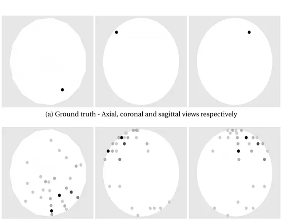
The first kind of experiment consisted of a set of ten simulations that have a sin-gle dipole active referred in the following as sinsin-gle dipole activations #1 through #10. With these activations, the localization error was found to be 0.00mm for all the dipoles with the three methods. The other performance parameters are displayed in Fig. 3.2showing the good performance of the proposed method (indicated by PM).

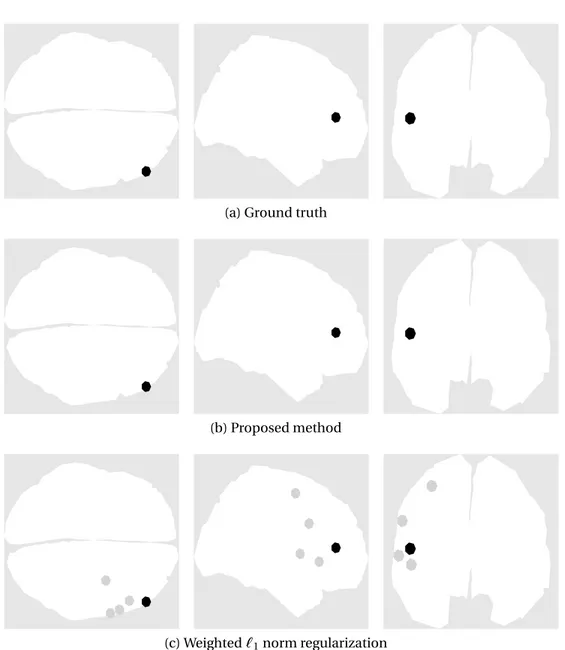
The brain activities detected by the proposed method and the weighted`1 norm solution are illustrated in Fig.3.3for a representative simulation. Our al-gorithm managed to perfectly recover the activity for 9 out of the 10 activations

20 30 40 1 2 3 4 5 6 7 8 9 10 0 2 4 sLoreta PM L1

(a) Center-mass localization error (mm)

40 50 1 2 3 4 5 6 7 8 9 10 0 5 10 sLoreta PM L1 (b) Excitation extension (mm) 60 70 1 2 3 4 5 6 7 8 9 10 0 5 10 15 sLoreta PM L1 (c) Transportation cost (mm)

Figure 3.2: Simulation results for single dipole experiments. The horizontal axis indicates the activation number. The error bars show the standard deviation over 12 Monte Carlo runs.

(a) Ground truth

(b) Proposed method

(c) Weighted`1norm regularization

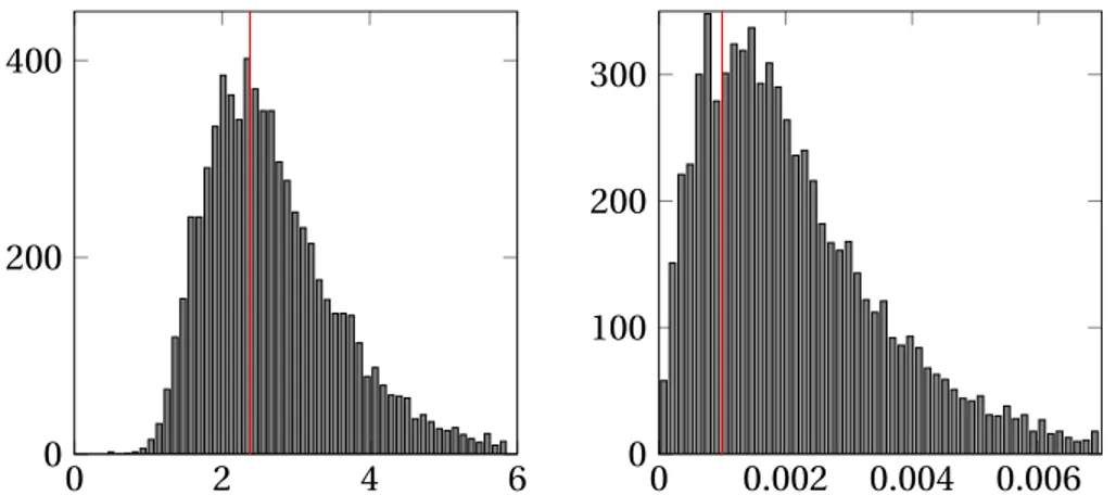
0 2 4 6 0

200 400

(a) Histogram ofσ2_n. Estimated mean value: 2.75. Ground truth: 2.38. 0 0.002 0.004 0.006 0 100 200 300

(b) Histogram of ω. Estimated mean value: 2.18e-3. Ground truth : 1.00e-3.

0 5 10 15

0 500 1,000

(c) Histogram of_{λ. Estimated mean value:} 8.36. 0.9 1 1.1 0 100 200 300 400

(d) Histogram of xi. Estimated mean value: 1.02. Ground truth: 1.00.

Figure 3.4: Histogram of samples generated by the MCMC method for one of the single dipole simulations. The estimated mean values and ground truth are indicated in the figures.

(with center-mass localization error, extension and transportation cost equal to 0.00mm) for all simulations. The dipole corresponding to activation #7 was located precisely for some simulations and with very reduced error in the oth-ers. The mean transportation cost of the proposed method for activation #7 is 0.7mm. In comparison, sLoreta has an excitation extension that is signifi-cantly larger (between 41mm and 51mm for the different dipole positions) (as expected for an`2norm regularization) and a larger transportation cost (bigger than 55mm in all cases). The weighted`1norm regularization provides better estimations than sLoreta with a mean extension of up to 10mm and transporta-tion cost of up to 13mm but is still outperformed by the proposed method.

In addition, Fig.3.4shows the histograms of the samples ofσ2_n,ω, λ and the amplitude of the active dipole xi j for one of the simulations corresponding to

simulation #3 as a representative case. It is shown that the ground truth values ofω (the proportion of non-zeros 1/1003), σ2_nand xi j are inside the support of

their histograms and are close to their estimated mean values, i.e., close to their minimum mean square error estimates.

3.4.1.4 MULTIPLE DISTANT DIPOLES

The second kind of experiments evaluates the performance of the proposed algorithm when several dipoles are activated at the same time in distant space positions. More precisely, we chose randomly the following sets of dipoles from the 1003 dipoles present in the head model

• (i) Two pairs of N = 2 simultaneous dipoles spaced more than 100mm (activations #1 and #2).

• (ii) Two sets of N = 3 simultaneous dipoles spaced more than 100mm (activations #3 and #4).

The brain activities associated with two representative simulations corre-sponding to two and three dipoles are illustrated in Figs. 3.5and3.6. The ac-tivation #2 associated with two distant dipoles displayed in Fig. 3.5is an inter-esting case for which the weighted`1 norm regularization fails completely to recover one of the dipoles. The activation #4 displayed in Fig. 3.6shows that the proposed method detects an activity more concentrated in the activated dipoles while the`1norm regularization provides less-sparse solutions.

Quantitative results in terms of transportation costs are displayed in Fig.

(a) Ground truth

(b) Proposed method

(c) Weighted`1norm regularization

Figure 3.5: Brain activity for a multiple distant dipole experiment (activation # 2 that has two active dipoles).

(a) Ground truth

(b) Proposed method

(c) Weighted`1norm regularization

Figure 3.6: Brain activity for a multiple distant dipole experiment (activation # 3 that has three active dipoles).

1 2 3 4 0 20 40 60 _PM L1 sLoreta

Figure 3.7: Transportation cost for multiple distant dipoles experiments, the horizontal axis indicates the activation number (1 and 2: two active dipoles, 3 and 4: three active dipoles). The error bars show the standard deviation over 12 Monte Carlo runs.

proposed method are below 3.6mm in all cases and are clearly smaller than those obtained with the other methods. Indeed, the sLoreta transportation costs are between 50 and 62mm, and the transportation costs associated with the weighted`1norm regularization are between 3.9mm and 13mm, except for the activation #2 where it fails to recover one of the dipoles as previously stated.

3.4.1.5 MULTIPLE CLOSE DIPOLES

The third kind of experiments evaluates the performance of the proposed al-gorithm for active dipoles that have close spatial positions. More precisely, we randomly chose the following sets of dipoles

• (i) Two pairs of dipoles spaced approximately 50 (activations #1 and #2). • (ii) Two pairs of dipoles spaced approximately 30mm (activations #3 and

#4).

• (iii) Two pairs of dipoles spaced approximately 10mm (activations #5 and #6).

Figure 3.8 compares the transportation costs obtained with the different methods. Since it is much harder to distinguish the activity produced by two

1 2 3 4 5 6 0 20 40 60 PM_L1 sLoreta (a)

Figure 3.8: Transportation cost for multiple close dipoles experiments. The hor-izontal axis indicates the activation number (1 and 2: 50mm separation, 3 and 4: 30mm separation, 5 and 6: 10mm separation). The error bars show the stan-dard deviation over 12 Monte Carlo runs.

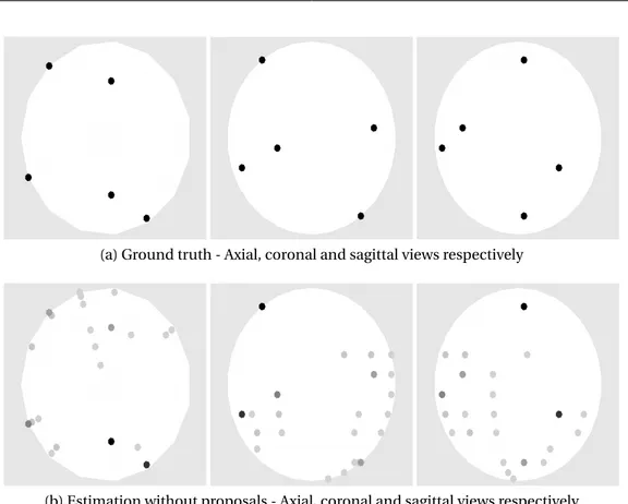
close dipoles, the transportation costs associated with the proposed method and the weighted `1 norm regularization are considerably higher than those obtained previously. However, the transportation costs obtained with the pro-posed algorithm are still below those obtained with the two other estimation strategies. Some interesting cases can be observed in Figs.3.9and3.10. Figure

3.9corresponds to one case where both algorithms fail to identify two dipoles and fuse them into a single dipole located in the middle of the two actual loca-tions. In this particular activation, our algorithm adds considerably less extra activity than the weighted`1norm regularization. In the case illustrated in Fig.

3.10, the proposed method correctly identifies two dipoles (but moves one of them from its original positions) while the weighted`1norm regularization es-timates a single dipole located very far from the two excited dipoles.

3.4.2

R

Two different sets of real data were considered. The first one consists of an auditory evoked response while the second one is the evoked response to facial stimulus. In addition to the weighted`1norm regularization, we also compared our results with the MSP algorithm [51] using the default parameters in the SPM

(a) Ground truth

(b) Proposed method

(c) Weighted`1norm regularization

Figure 3.9: Brain activity for multiple close dipoles (activation # 4 that has a 30mm separation between dipoles).

(a) Ground truth

(b) Proposed method

(c) Weighted`1norm regularization

Figure 3.10: Brain activity for multiple close dipoles (activation # 6 that has a 10mm separation between dipoles).

software.2

3.4.2.1 AUDITORY EVOKED RESPONSES

The used data set was extracted from the MNE software [79,80]. It corresponds to an evoked response to left-ear auditory pure-tone stimulus using a realistic BEM head model. The data was acquired using 60 EEG electrodes sampled at 600 samples/s. The samples were low-pass filtered at 40Hz and downsampled to 150 samples/s. The noise covariance matrix was estimated from 200ms of data preceding each stimulus and was used to whiten the data. Fifty one epochs were averaged to generate the measurementsY.

The sources associated with this example are composed of 1844 dipoles located on the cortex with orientations that are normal to the brain surface. One channel that had technical artifacts was ignored resulting in an operator

H∈ R59×1884. We processed the eight time samples corresponding to 80ms ≤ t ≤ 126ms, i.e., associated with the highest activity period in the M/EEG mea-surements as displayed in Fig.3.11.

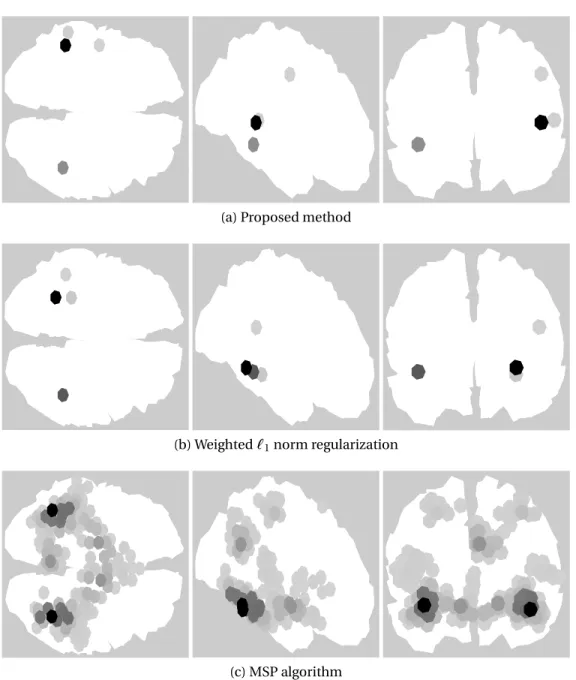
The sum of the estimated brain activities over the 8 time samples obtained by the proposed method, the weighted `1 norm regularization and the MSP algorithm are presented in Fig. 3.12. The proposed method consistently de-tects most of the activity concentrated in both the ipsilateral and contralateral auditory cortices. The weighted`1norm regularization detects the activity in the right cortex in a similar position, but moves the activity detected in the left cortex to a lower point of the brain that is further away from the auditory cor-tex. The MSP algorithm finds the activity correctly in the auditory cortices but spreads it around a region instead of focusing it on a small number of dipoles. This is due to the fact that both the proposed method and the weighted `1 norm promote sparsity over the dipoles while MSP promotes sparsity over pre-selected brain regions that depend on the parcellation scheme used.

3.4.2.2 FACE-EVOKED RESPONSES

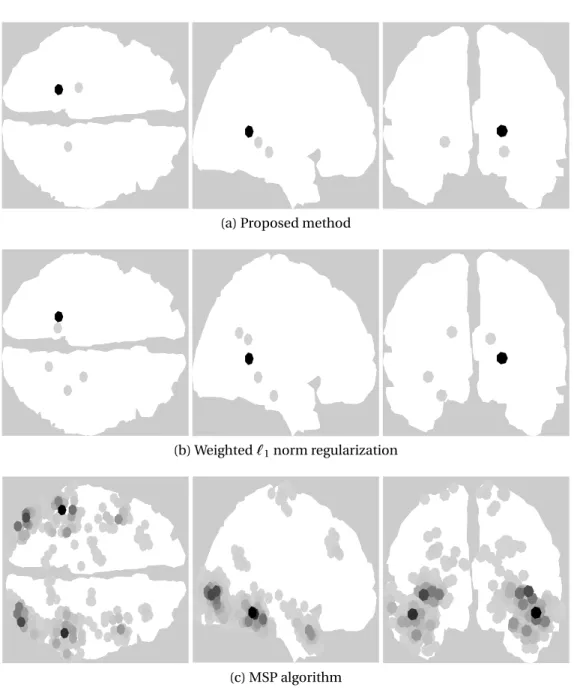
The data used in this section is one of the sample data sets available in the SPM software. It was acquired from a face perception study in which the subject had to judge the symmetry of a mixed set of faces and scrambled faces. Faces were presented during 600ms with an interval of 3600ms (for more details on the

0 20 40 60 80 100 120 140 160 180 200 −6,000 −4,000 −2,000 0 2,000 4,000 6,000 Time (ms) Whiten ed amp lit u de

(a) Proposed method

(b) Weighted`1norm regularization

(c) MSP algorithm

Figure 3.12: Brain activity for the auditory evoked responses from 80ms to 126ms.

(a) Proposed method

(b) Weighted`1norm regularization

(c) MSP algorithm