ÉCOLE DE TECHNOLOGIE SUPÉRIEURE UNIVERSITÉ DU QUÉBEC
MANUSCRIPT-BASED THESIS PRESENTED TO L’ÉCOLE DE TECHNOLOGIE SUPÉRIEURE
IN PARTIAL FULFILLMENT OF THE REQUIREMENTS FOR THE DEGREE OF DOCTOR OF PHILOSOPHY
Ph.D.
BY
Fernando José QUEVEDO GONZÁLEZ
COMPUTATIONAL DESIGN OF FUNCTIONALLY GRADED HIP IMPLANTS BY MEANS OF ADDITIVELY MANUFACTURED POROUS MATERIALS
MONTREAL, JUNE 23RD, 2016
This Creative Commons licence allows readers to dowload this work and share it with others as long as the author is credited. The content of this work may not be modified in any way or used commercially.
BOARD OF EXAMINERS (THESIS PH.D.) THIS THESIS HAS BEEN EVALUATED BY THE FOLLOWING BOARD OF EXAMINERS:
Dr. Natalia Nuño, thesis supervisor
Department of Automated Manufacturing Engineering at École de technologie supérieure
Dr. Vincent Demers, president of the committee
Department of Mechanical Engineering at École de technologie supérieure
Dr. Farid Amirouche, external examiner
Department of Mechanical and Industrial Engineering at University of Illinois at Chicago
Dr. Patrick Terriault, member of the committee
Department of Mechanical Engineering at École de technologie supérieure
THIS THESIS WAS PRESENTED AND DEFENDED
IN THE PRESENCE OF A BOARD OF EXAMINERS AND THE PUBLIC JUNE 8TH, 2016
ACKNOWLEDGEMENTS
I face now the time where I look back and realize how thankful I have to be, since without the help, support and comfort from those who have been around me, I wouldn’t be able to accomplish this task. I apologize if you don’t see yourself amongst these lines, but be sure that if we shared something during these years, you certainly left a trace and I’m deeply thankful to you for that. I would like to start by thanking God for the roads He has driven me through and the ones that He will bring me to.
Natalia MERCI en majuscules tout d’abord de m’avoir fait confiance et donné la chance de pouvoir faire le doctorat. Si je suis où je suis c’est en grande part grâce à toi! Merci de ta façon de me guider, sans chercher à t’imposer; de tes commentaires et suggestions, toujours dites de la meilleure façon possible. Merci aussi d’avoir un œil sur le plan académique et un autre sur le personnel car on a toujours besoin de quelqu’un à l’écoute.
Papá, Mamá, Irene GRACIAS por vuestro apoyo, por tantas veces en las que me escucharon aun sin llegar a comprender, por estar ahí siempre, en los buenos momentos y cuando las cosas han sido más complicadas. Aun estando lejos, vuestra presencia me ha mantenido a flote. Es gracias a ustedes que he llegado hasta aquí y es por ustedes que lo he hecho. Mi mayor placer es que ustedes estén orgullosos de mí.
Audrey, merci de tout ton soutien, de ton écoute, de ta préoccupation pour moi. Merci de tes conseils, de tes corrections… Merci surtout de tant des bons moments, d’avoir été un support dans lequel m’appuyer, de chercher à enlever mes préoccupations et de me motiver quand j’en avais besoin.
Micke, merci d’avoir supporté mon français lorsque je ne le parlais presque pas. Merci d’avoir été toujours disponible pour lire et corriger mes rapports, d’être à l’écoute et chercher à aider. Ça a été une chance de pouvoir travailler avec toi et d’apprendre de toi, mais surtout d’avoir trouvé en toi plus qu’un collègue de bureau.
Roland, merci de m’avoir fait confiance pour donner des travaux pratiques, ce qui m’a fait grandir et merci aussi de tes passages au labo que j’apprécie toujours autant.
Phillipe, merci de tes commentaires toujours si pertinents, de tes idées cherchant toujours améliorer un projet que t’as pris comme le tien et merci de le faire connaître là où tu vas. Nicolas, merci de ton énorme contribution à la suite de ce projet. Travailler à tes cotés a été un apprentissage continu. Jiaquiang merci de ta disponibilité pour les essais mécaniques et du temps sans mesure que tu as dédié. Merci Isabelle, j’ai bien apprécié ta façon de travailler, ta réceptivité aux commentaires et tu as fait une grande contribution à la suite du projet. Anthony Barraud et Erwan Jouault, merci de votre contribution qui a fait avancer le projet.
Merci à Justine, Félix, Lauranne, Michelle, Pierre-Olivier, Ali, Julien, Christiane, Olivier, Léon, et d’autres membres du LIO avec qui j’ai eu la chance de partager des moments et de qui j’ai pu apprendre.
Alejandro, gracias! Tú fuiste la persona con la que descubrí el gusto por la investigación y la biomecánica. Siempre te estaré agradecido por tu cercanía, tu saber hacer y por tanto que aprendí contigo. Has pasado de ser mi profesor a un colaborador al que admiro, un amigo al que aprecio. Gracias siempre estar dispuesto a colaborar.
Merci à Charles Simoneau, Vladimir Brailovski et autres membres du LAMSI ainsi qu’à M. Éric Lavoie de l’IREQ pour sa participation es ses conseils en la fabrication d’échantillons. Merci Dominique Grenier et Youri Juteau pour avoir toujours été si disponibles lorsqu’on a eu besoin de faire des prototypes.
Thanks to Roger and Justine, we need true friends to overcome the hard days and to enjoy the good ones and you have become these good friends to me. Finalmente, gracias a mis amigos por el mundo, los que siempre están ahí y que tengo muy presentes en cada paso que doy.
COMPUTATIONAL DESIGN OF FUNCTIONALLY GRADED HIP IMPLANTS BY MEANS OF ADDITIVELY MANUFACTURED POROUS MATERIAL
Fernando José QUEVEDO GONZÁLEZ
ABSTRACT
Two of the main mechanically related problems of hip implants are the bone resorption due to the reduction of the stresses in the bone caused by the presence of the implant (stress shielding), and the interfacial failure caused by inadequate stress distribution at the bone-implant interface. While stiff bone-implants increase stress shielding, flexible bone-implants cause higher contact interfacial stresses. A compromise is thus needed, and two design strategies have been suggested: 1) optimize the hip implant shape, or 2) optimize the functional gradation of mechanical properties of the implant. Additive manufacturing (AM) allows for the fabrication of implant shapes with almost no restrictions, and the production of porous materials whose mechanical properties are dependent on their geometrical parameters, which can be controlled. Therefore, AM allows for the production of implants having optimized shape and optimized functional gradation of mechanical properties. In addition, AM allows for quick design modifications and the possibility of patient-specific implants.
This thesis aims at taking advantage of the capabilities offered by AM for the design of the shape and functional gradation of the mechanical properties of hip stems in order to improve the mechanical compatibility with the bone (i.e. reduce the stress shielding and generate adequate interfacial stresses). To this end, finite element (FE) models are used to predict the mechanical behavior of the porous materials when designing hip stems. In a first step, the cost-effectiveness of the FE modeling approach for porous materials (e.g. beam or solid finite elements and sample size choice) was evaluated. In a second step, the irregularities that arise during the manufacturing process (e.g. strut inclination, strut diameter variation and strut elimination) were included in the FE model in order to enhance the correlation with experimental data. In the third part of this work, the shape and distribution of mechanical properties of a hip stem were optimized in order to reduce the bone loss and generate adequate interfacial stresses. The FE model of the porous material developed in the previous steps was then used to obtain the optimized distribution of mechanical properties of the stem. The present work provides a methodology for obtaining accurate predictions of the mechanical behavior of AM porous materials. Furthermore, it provides a framework to conceive optimized hip implants having enhanced mechanical compatibility with the bone and produced with AM. To this end, optimized shape is combined with porous materials to achieve a functional gradation of the mechanical properties of the implants.
Keywords: hip stem optimization, functionally graded implants, additive manufacturing,
CONCEPTION NUMÉRIQUE D’IMPLANTS DE HANCHE AVEC DES
PROPRIÉTÉS MÉCANIQUES GRADUÉES À L’AIDE DES MATÉRIAUX POREUX PRODUITS PAR FABRICATION ADDITIVE
Fernando José QUEVEDO GONZÁLEZ
RÉSUMÉ
Deux des principaux problèmes des implants de la hanche ayant une origine mécanique sont la résorption osseuse causée par une réduction de contraintes dans l'os suite à la présence de l'implant (protection des contraintes) et l’échec à l’interface dû à une distribution inadéquate des contraintes de contact. Des implants rigides contribuent à la protection des contraintes, tandis que des implants flexibles causent des contraintes de contact plus élevées. Afin de trouver un compromis, deux approches ont été proposées: optimiser la forme ou optimiser la gradation fonctionnelle des propriétés mécaniques de l’implant. La fabrication additive (FA) permet de produire presque n'importe quelle forme d'implant, ainsi que de fabriquer des matériaux poreux, dont les propriétés mécaniques dépendent de leur structure, qui peut être contrôlée. Il est donc possible d’obtenir des implants avec une géométrie et une gradation des propriétés mécaniques optimisées. De plus, la FA permet de faire des changements instantanés dans le design, permettant la conception d’implants sur mesure.
Cette thèse vise à exploiter les possibilités de la FA pour la conception d'implants ayant une forme et une gradation des propriétés mécaniques optimisées afin d'améliorer la compatibilité mécanique de l'implant avec l’os (i.e. réduire la protection de contraintes et générer des contraintes à l’interface adéquates). Des modèles éléments finis (ÉF) ont été utilisés pour évaluer le comportement mécanique du matériau poreux ainsi que pour concevoir la tige de hanche. Dans un premier temps, l’approche pour la modélisation par ÉF des matériaux poreux (modèles de poutres ou solides, choix de la taille de l’échantillon) a été évaluée en termes de son rapport coût-efficacité. Ensuite, les imperfections dues à la fabrication des matériaux poreux (inclination, variation du diamètre et élimination des barreaux) ont été incluses dans les modèles ÉF précédents afin d'améliorer la correspondance avec les données expérimentales. Enfin, la forme et la distribution des propriétés mécaniques de l’implant de la hanche ont été optimisées afin de réduire la perte osseuse et générer une distribution adéquate des contraintes à l’interface. Le modèle ÉF du matériau poreux développé dans les étapes précédentes a servi à obtenir la distribution optimisée des propriétés mécaniques dans la tige.
Le présent travail fournit un outil pour évaluer avec une bonne précision le comportement mécanique des matériaux poreux produits par FA. De plus, il explore l’amélioration de la compatibilité mécanique obtenue avec des implants de la hanche conçus dans l’optique de la FA, et il développe une méthodologie pour l’optimisation des implants en termes de sa forme et de la distribution de ses propriétés mécaniques, obtenue à l’aide des matériaux poreux.
Mots clés: optimisation des implants de la hanche, implants gradées fonctionnellement,
TABLE OF CONTENTS
Page
INTRODUCTION ...1
CHAPTER 1 GENERAL CONCEPTS AND LITTERATURE REVIEW ...5
1.1 The biomechanics of the femur at the hip joint ...5
1.1.1 Anatomy ... 5 1.1.2 Forces ... 7 1.1.3 Mechanical properties ... 8 1.1.3.1 Elastic modulus ... 10 1.1.3.2 Strength ... 10 1.1.3.3 Interfacial strength ... 10
1.2 Total hip arthroplasty ...11
1.2.1 Epidemiology and future perspectives ... 13
1.2.2 Main related problems ... 14
1.3 Numerical analysis of hip implants...15
1.3.1 Mechanical causes of implant failure ... 15
1.3.1.1 Stress shielding ... 15
1.3.1.2 Interfacial failure ... 17
1.3.2 Improvement of stem performance ... 18
1.3.2.1 Optimization of implant shape ... 18
1.3.2.2 Functionally graded stems ... 20
1.4 Porous materials ...22
1.4.1 Well-ordered porous materials ... 23
1.4.2 Main geometrical parameters of porous materials ... 24
1.4.3 Additive manufacturing of porous materials ... 25
1.4.3.1 Irregularities of additively manufactured porous materials ... 27
1.4.3.1.1 Contribution related to this thesis ... 28
1.4.4 Mechanical properties of porous materials ... 28
1.4.4.1 Experimental testing of porous materials ... 29
1.4.4.2 Numerical modeling ... 32
1.4.4.2.1 Effect of manufacturing irregularities ... 35
1.5 Summary ...36
CHAPTER 2 HYPOTHESIS, OBJECTIVES AND STRUCTURE OF THE THESIS ...37
2.1 Problem statement ...37
2.2 Hypothesis and objectives...38
CHAPTER 3 ARTICLE 1. FINITE ELEMENT MODELLING APPROACHES FOR WELL-ORDERED POROUS METALLIC MATERIALS FOR ORTHOPAEDIC APPLICATIONS: COST EFFECTIVENESS AND GEOMETRICAL CONSIDERATIONS ...43
3.1 Abstract ...43
3.3 Materials and Methods ...46
3.3.1 Geometrical parameters at mesoscale ... 47
3.3.2 Finite element (FE) modelling approaches ... 48
3.3.2.1 Finite size solid FE model ... 49
3.3.2.2 Finite size beam FE model ... 50
3.3.2.3 Infinite media model ... 51
3.3.3 Performed FE analyses ... 52
3.3.3.1 Determination of the cost-effective model approach ... 52
3.3.3.2 Unit cell geometry comparison: cubic and diamond ... 53
3.3.3.3 Criteria 1: similar bending and compressive behaviours ... 53
3.3.3.4 Criteria 2: mechanical properties close to bone ... 54
3.3.3.5 Criteria 3: Stress distribution uniformity within struts ... 54
3.4 Results ...54
3.4.1 Determination of the cost-effective model approach ... 54
3.4.2 Unit cell geometry comparison: cubic and diamond ... 57
3.4.2.1 Criteria 1: similar bending and compressive behaviours ... 57
3.4.2.2 Criteria 2: mechanical properties close to bone ... 58
3.4.2.3 Criteria 3: stress distribution uniformity within struts ... 59
3.5 Discussion ...60
3.6 Conclusion ...62
3.7 Acknowledgements ...63
CHAPTER 4 ARTICLE 2. FINITE ELEMENT MODELING OF MANUFACTURING IRREGULARITIES OF POROUS MATERIALS ...65
4.1 Abstract ...65
4.2 Introduction ...66
4.3 Materials and Methods ...68
4.3.1 Experimental data ... 68
4.3.2 FE modeling ... 69
4.3.3 Characterization and implementation of manufacturing irregularities in the FE model ... 71
4.3.3.1 Strut diameter variation ... 71
4.3.3.2 Strut inclination ... 72
4.3.3.3 Fractured struts ... 73
4.3.4 Finite Element Analyses ... 73
4.4 Results ...74
4.4.1 Characterization of manufacturing irregularities ... 74
4.4.2 Finite element analyses ... 75
4.4.3 Influence of the three geometrical irregularities for set S450P700 ... 75
4.4.4 Simulation of the other sample sets ... 78
4.5 Discussion ...80
4.6 Conclusions ...82
CHAPTER 5 ARTICLE 3. NUMERICAL DESIGN OF HIP STEMS WITH OPTIMIZED SHAPE AND FUNCTIONALLY GRADED MATERIAL PROPERTIES BY MEANS OF ADDITIVE MANUFACTURED
POROUS MATERIALS ...83
5.1 Abstract ...83
5.2 Introduction ...84
5.3 Materials and Methods ...86
5.3.1 Optimization strategy ... 86
5.3.1.1 Stem optimization at the macroscale ... 87
5.3.1.2 Porous material tailoring at the mesoscale ... 90
5.3.2 Finite element modeling ... 91
5.3.2.1 Stem and bone at the macroscale ... 91
5.3.2.2 Porous material at the mesoscale ... 92
5.4 Results ...93
5.5 Discussion ...97
5.6 Conclusion ...100
5.7 Acknowledgements ...100
CHAPTER 6 GENERAL DISCUSSION ...101
6.1 Synthesis of the articles ...102
6.2 Limitations ...103
6.2.1 Limitations related to the porous material model ... 103
6.2.1.1 Unit cell geometry ... 103
6.2.1.2 Beam model ... 104
6.2.1.3 Manufacturing irregularities ... 105
6.2.2 Limitations related to the optimization of the hip stem ... 105
6.2.2.1 Dimensionality of the bone-implant model ... 106
6.2.2.2 Interfacial conditions ... 106
6.2.2.3 Evaluation of implant performance ... 107
6.2.2.4 Tailoring of the porous material ... 107
6.3 Future work ...108
CONCLUSION ...111
APPENDIX I EXPERIMENTAL TESTS OF POROUS MATERIALS ...113
APPENDIX II BRENT’S METHOD FOR ROOT FINDING ...115
APPENDIX III NSGA-II GENETIC ALGORITHM, SIMULATED BINARY CROSSOVER AND POLYNOMIAL MUTATION ...117
AIII.1 The evolution process ...118
AIII.2 Tournament selection ...119
AIII.3 Genetic operators ...119
AIII.3.1 Simulated binary crossover ... 119
LIST OF TABLES
Page Table 1.1 Muscle forces (in % of the bodyweight) and their representation for stair
climbing. ...8
Table 1.2 Differences between EBM and DSLM technologies ...27
Table 1.3 Relationship between the elastic modulus and the relative density for different unit cells. Analytical relationships are indicated by * ...32
Table 3.1 Performed analyses ...46
Table 3.2 Geometrical parameters at the mesoscale used in the FE analyses. ...52
Table 3.3 Comparison between Eap,comp and Eap,bend for the two unit cell geometries and different SR using np=8. ...58
Table 3.4 Comparison of vap for the two unit cell geometries and different SR using np=8 ...59
Table 4.1 Design and experimental strut and pore sizes ...69
Table 4.2 Measured strut inclination (Sinc) and fractured struts (Sfr) manufacturing irregularities of non-tested sample S450P700. ...74
Table 5.1 Initial, minimum and maximum values for the 8 shape variables ...89
Table 5.2 Values for the distributions of manufacturing irregularities ...92
LIST OF FIGURES
Page
Figure 0.1 General schema of the thesis ...3
Figure 1.1 The femur. ...6
Figure 1.2 (a) The hip joint and its movements (adapted from (Tortora 2012)); (b) reference system of the femur ...7
Figure 1.3 Cortical and cancellous bone ...9
Figure 1.4 Total hip replacement components. ...12
Figure 1.5 (a) Anatomical, (b) cylindrical and (c) tapered cementless stems. The hatched represents the porous coated zone for bone ingrowth. ...13
Figure 1.6 Causes for revision of the arthroplasty in Canada ...15
Figure 1.7 Interfacial failure index for (a) solid titanium and (b) flexible stems. ...17
Figure 1.8 (a) Bone density after remodeling and (b) interfacial failure around a stem with optimized shape. ...19
Figure 1.9 (a) Porous material density distribution; (b) bone resorption; (c) interfacial shear stresses for a functionally graded hip stem; (d) bone resorption; (e) interfacial shear stresses for a solid Ti6Al4V stem. Adapted from Arabnejad Khanoki and Pasini (2013c) ...21
Figure 1.10 Macroscale, mesoscale and microscale of a porous material ...23
Figure 1.11 (a) Simple cubic and (b) diamond unit cells ...24
Figure 1.12 The process of additive manufacturing. Taken from (Heinl, et al. 2008) ...26
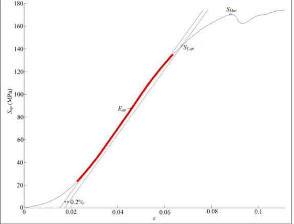
Figure 1.13 Computation of apparent mechanical behavior from the results of an experimental compression test. Apparent linear zone stands in red ...29
Figure 1.14 Reported values of Eap of Ti6Al4V porous materials ...30
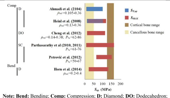
Figure 1.15 Reported values of SY,ap and SMAX of Ti6Al4V porous materials ...31
Figure 1.16 Simple cubic unit cell: (a) continuum model (solid FE elements); (b) 3-node beam model (1 element per strut) ...33
Figure 3.1 Cubic (a) and diamond (b) unit cell geometries showing main parameters ...47
Figure 3.2 Symmetry surfaces and loading application of the solid FE model ...50
Figure 3.3 Periodic boundary conditionsused for the 3D Infinite media approach ...51
Figure 3.4 Eap,comp as a function of np (from 2 to 10) for the cubi unit cell geometry using the solid, beam and infinite media FE models (ϕS = 450 µm) ...55
Figure 3.5 |ΔEap,comp| as a function of Δnp (variation of Eap,comp for np ...56
Figure 3.6 ε% (difference in Eap,comp as between solid and beam FE models) a function of SR (ϕS = 450 μm) for np = 8 ...57
Figure 3.7 (a) Stress distribution within the struts for the cubic unit cell geometry; and (b) diamond unit cell geometry; (c) pure compression zones (in red) for the cubic unit cell geometry; (d) pure compression (in red) and (e) pure traction zones (in green), respectively, for the diamond unit cell geometry ...60
Figure 4.1 (a) Cubic unit-cell pore geometry and main parameters and (b) 10-pore sample model generated by periodic repetitions of the unit-cell ...68
Figure 4.2 Different types of geometrical manufacturing irregularities: strut diameter variation (solid points), strut inclination (straight lines) and fractured struts (empty circles) ...70
Figure 4.3 Schematization of the strut diameter variation ...71
Figure 4.4 Conversion of diameter value to section number ...72
Figure 4.5 Conversion of the inclination angle θ to keypoint shifting distance ...73
Figure 4.6 Apparent stress-compressive strain (σap-ε) curves for the set S450P700 obtained with the idealized model, the different combinations of manufacturing irregularities, and the experimental tests. Dvar: diameter variation; Sfr: fractured struts; Sinc: inclined struts; Exp: experimental ...76
Figure 4.7 Eap and SY,ap obtained with the idealized model, the different combinations of manufacturing irregularities, and the experimental tests for the set S450P700. Dvar: diameter variation; Sfr: fractured struts; Sinc: inclined struts; Exp: experimental. ...78
Figure 4.8 Comparison of SY,ap (plain bars) and Eap (hatched bars) obtained from
experimental tests (Exp) and from FE simulations including the three manufacturing irregularities (Sim) for the three sets (S450P600, S450P700 and S450P800) ...79 Figure 5.1 General schema for the functionally graded stem optimization. ...86 Figure 5.2 Geometrical variables (hj) for the stem shape and grid (red dots) for the
optimization of material properties. The angles α1=29.79°, α2=15.8°,
α3=4.88° have fixed values ...88
Figure 5.3 Meshing and loading of the stem and bone model ...91 Figure 5.4 Porous material model at the mesoscale: a - idealized; b - with manufacturing
irregularities. Beam elements have been thickened to show the ϕS variation ..93
Figure 5.5 590 optimized stems after 50 generations (30090 function evaluations). Diamond markers: first non-dominated front. The different plots show the influence of bone resorption, stem size, stiffness and length in the interfacial failure index (FIS) and bone loss index (FBL). Representative
selected stem designs b-e are circled ...94 Figure 5.6 Distribution of resorbed bone (grey) and non-resorbed bone (black) and
interfacial shear stresses (in MPa) for a) the original stem design; b)-e) the selected (optimized) stem designs of Figure 5.5. The color maps represent the strut thickness (ϕS in mm) and the corresponding apparent elastic
modulus (Eap, in GPa) as computed in the porous material tailoring at the
mesoscale step ...96 Figure 5.7 Differences (in %) between Eap and the prescribed E for the selected stem
designs b – e of Figure 5.5. ...97 Figure AII.1 Sorting of the current population and creation of the parent population for
LIST OF ACRONYMS
2D Two dimensions
3D Three dimensions
ANOVA Analysis of variance
BCC Body centered cubic unit cell
Bend Bending
CAD Computer aided design
CoCrMo Cobalt-Chrome-Molybdenum alloy
Comp Compression
D Diamond unit cell
dir1, dir2 Direction 1, 2
DO Dodecahedron unit cell
DMLS Direct metal laser sintering
DT Dode-thin unit cell
Dvar Strut diameter variation
EBM Electron Beam Melting
Exp Experimental value for the mechanical behavior of the porous material
FE Finite element
FEA Finite element analysis
FG Functionally graded
gen Generation of the genetic algorithm
GY Gyroid unit cell
IBV Biomechanic’s Institute of Valence (Instituto de Biomecánica de Valencia), Spain
MP Material properties
NSERC Natural Sciences and Engineering Research Council of Canada
NSGA-II Non-dominated sorted genetic algorithm II
PM Polynomial mutation
OA Osteoarthritis
RMSD Root mean square difference
SC Simple cubic unit cell
SBX Simulated binary crossover
Sfr Fractured struts
Sim Simulated value for the mechanical behavior of the porous material
Sinc Strut inclination
SLM Selective laser melting
THA Total hip arthroplasty
LIST OF SYMBOLS
A Area of the cross-section of the strut (µm2) Astem Interfacial area of the stem (mm2)
C1 Constant relating the apparent elastic modulus to the density of the porous
material
dAstem Differential of stem interfacial area
dVbone Differential of bone volume
E Elastic modulus (GPa)
Eap Apparent elastic modulus of the porous material (GPa)
Eap,beam Apparent elastic modulus of the beam model (GPa)
Eap,bend Apparent elastic modulus in bending of the porous material (GPa)
Ecanc Elastic modulus of the cancellous bone (GPa)
Eap,comp Apparent elastic modulus in compression of the porous material (GPa)
ΔEap,comp Variation in Eap,comp for a 1 pore increase in the sample size (GPa)
Eap,dir1 Apparent elastic modulus of the porous material in direction 1 (GPa)
Eap,dir2 Apparent elastic modulus of the porous material in direction 2 (GPa)
Eap,solid Apparent elastic modulus of the solid (continuum) model (GPa)
Ecort Elastic modulus of the cortical bone (GPa)
Ei Elastic modulus the stem material optimization point i (GPa)
Emax Maximum elastic modulus for the stem material optimization (GPa)
Emin Minimum elastic modulus for the stem material optimization (GPa)
ES Elastic modulus of the solid phase of the porous material (GPa)
Fabd Abductor muscle force (N)
FBL Function of the bone loss (N)
Fcont Hip contact force (N)
fIS Local interfacial failure index
FIS Global interfacial failure index
Fvl Vastus lateralis muscle force (N)
Fvm Vastus medialis muscle force (N)
G Shear modulus (GPa) g(Sen) Bone resorption function
hj Shape variable j of the stem (mm)
hj,max Maximum value of the shape variable j of the stem (mm)
hj,min Minimum value of the shape variable j of the stem (mm)
I Counter
I Inertia of the cross-section of the strut (µm4) Iap Apparent inertia of the porous material (µm4)
K Tangent modulus (GPa) Ki,, Keypoint
L Length of the strut (µm)
Lcell, LUC Length of the unit cell (µm, mm)
Lcell,cubic Length of the simple cubic unit cell (µm)
Lcell,diamond Length of the diamond unit cell (µm)
Lsample Porous material sample length (mm)
mloss,stem Bone loss (resected) due to the stem insertion (mg)
mr Resorbed bone mass fraction
ms Mass of the porous material (mg)
nmppt Number of stem material optimization points np Number of unit cells
Δnp Increment of the number of unit cells
P% Porosity
Sbone Strength of the bone (MPa)
Sc Interfacial compression strength (MPa)
sd Dead zone parameter
Sen Strain energy per unit of bone mass (mJ/mg)
Sen,ref Reference strain energy per unit of bone mass (mJ/mg)
SMax Maximum (apparent) strength of the porous material (MPa)
Sn Section number
SR Slenderness ratio
SS Interfacial shear strength (MPa)
St Interfacial traction strength (MPa)
SY Yield strength (MPa)
SY,ap Apparent yield strength of the porous material (MPa)
tol Tolerance
U Strain energy density (mJ/mm3) Δu Displacement (mm)
uij Directional degree of freedom (mm)
UN Normal degree of freedom (mm)
uvj Vertex directional degree of freedom (mm)
Vapp Apparent volume of the porous material (mm3)
Vbone Volume of the bone (mm3)
Vpores Volume of the void phase of the porous material (mm3)
Vsolid Volume of the solid phase of the porous material (mm3)
Greek symbols
αi Angle for defining the shape of the stem (°)
Δ Keypoint shifting distance (µm)
ε Strain (mm/mm)
ε% Difference between solid and beam models
θ Inclination angle (°) µ Mean value
µD Mean strut diameter (µm)
v Poisson’s ratio
vap Apparent Poisson’s ratio of the porous material
ρ Density of the bone (mg/mm3)
ρapp Apparent density of the porous material (mg/mm3)
ρr Relative density
ρS Density of the solid phase of the porous material (mg/mm3)
τ Shear interfacial stress (MPa) ϕdesign Designed strut diameter (µm)
ϕmin, ϕS,min Minimum strut diameter (µm)
ϕP Pore diameter (µm)
ϕrand Random strut diameter (µm)
ϕS Strut diameter (µm)
ϕS,max Maximum strut diameter (µm)
σ Standard deviation
σap Apparent stress of the porous material (MPa)
σAVG Average (von Mises) stress (MPa)
σN Normal interfacial stress (MPa)
σMAX Maximum (von Mises) stress (MPa)
INTRODUCTION
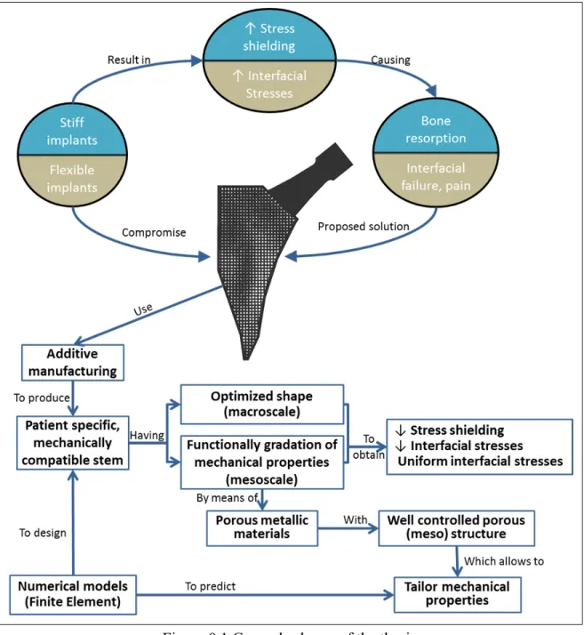
Hip arthroplasty is a successful procedure for relatively old patients. However, when it comes to younger and more active patients, the outcomes of this procedure are not as good (Swedish Hip Arthroplasty Register 2013, Canadian Institute for Health Information 2015, UK National Joint Registry 2015). Indeed, younger patients need implants (stems) that can not only withstand the increased loads derived from a more demanding physical activity, but also that can last longer (Kurtz, et al. 2009). In addition, the implant shall conserve as much bone stock as possible for an eventual revision. Implant shape and material properties have an impact on these requirements. For instance, large implants may provide great stability, but require more bone resection; on the other hand, smaller implants may improve the stress distribution in the proximal femur, but their stability is usually decreased (Reimeringer, et al. 2013) and the stresses at the bone-implant interface are much higher (Kuiper and Huiskes 1992). On the other hand, while stiff implants cause stress shielding (i.e. reduction of the stresses) of the bone that may lead to its resorption, more flexible implants have been shown to increase the interfacial stresses (Figure 0.1), with the associated increase in the risk of interfacial failure and pain (Kuiper and Huiskes 1992, 1997).
Two strategies have been proposed to simultaneously solve the above problems (decrease stress shielding and obtain appropriate interfacial stresses): 1) optimize the implant shape (Ruben, et al. 2012, Fernandes, et al. 2004, Chanda, et al. 2015), or 2) generate a gradation of the material properties of the stem (Kuiper and Huiskes 1997, Hedia, et al. 2006, Arabnejad Khanoki and Pasini 2012). Additive manufacturing technologies show few restrictions in terms of the shapes that can be produced. This allows the fabrication of porous materials with mechanical properties tailored to certain specifics by simply adjusting their (meso) structure (Figure 0.1). As a result, implants can now be created having the aforementioned optimized shape and gradation of mechanical properties, in order to decrease the effects of stress shielding (bone resorption) and the risks associated with inadequate interfacial stress distribution (failure and pain). Furthermore, with additive manufacturing design changes can be easily introduced, allowing for patient-specific design of hip implants (Figure 0.1).
In order to fully take advantage of these possibilities offered by additive manufacturing for implant design, it is necessary 1) to develop computational models to accurately evaluate the mechanical behavior of porous materials so that these can be tailored, and 2) develop a strategy for the optimization of the shape and material properties distribution of the implants (Figure 0.1) in order to improve their mechanical compatibility with the bone.
The main objective of this thesis is to develop a methodology for the design of a new generation of hip implants taking advantage of the various manufacturing capabilities offered by additive manufacturing technologies. In this way, additive manufactured porous materials are considered for obtaining a gradation in the mechanical properties of the stem such that the stress shielding is reduced and adequate interfacial stresses are obtained. The thesis is divided in three parts aiming, respectively, at 1) determining the cost-effective modeling approach for porous materials, 2) increasing the accuracy of computational model of additive manufactured porous materials, and 3) optimizing a hip stem made of porous materials. For all three parts, computational models were developed.
The present thesis is divided into six chapters. Chapter 1 presents a general literature review about the biomechanics of the femur, the hip implants and porous materials. Chapter 2 aims at formulating the main and specific objectives of the present thesis. Then the chapters 3, 4 and 5 comprise the three articles that attempt to address the proposed problem by answering each specific objective. Chapter 6 provides a summary of the results, and highlights the advantages and limitations of the present thesis, offering some recommendations for future work. A general conclusion follows.
CHAPTER 1
GENERAL CONCEPTS AND LITTERATURE REVIEW
This thesis relies on concepts from engineering and medicine. More particularly, the context of the problem being solved belongs to the medical field: improving the hip arthroplasty. On the other hand, the tools and concepts that provide the proposed solution are derived from the mechanical engineering and optimization principles: material mechanical behavior, porous materials and hip stem design optimization. This chapter aims at introducing the basic concepts from these disciplines to facilitate the understanding of the thesis. This chapter is structured as follows: first the biomechanics of the femur at the hip joint is depicted; second, the hip arthroplasty is presented; third the numerical analyses and optimization of hip stems are presented; fourth, the porous materials are described.
1.1 The biomechanics of the femur at the hip joint 1.1.1 Anatomy
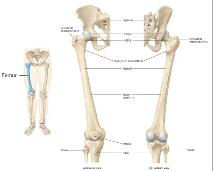
The femur goes from the hip to the knee, and is the longest bone of the body. It has an almost-cylindrical shape in its central portion (diaphysis). Proximally, the almost-spherical head of the femur articulates with the congruent surface of the pelvic acetabulum, forming the hip joint (Figure 1.1). This joint can be seen as a ball-and-socket (or spheroidal) union that has good range of tridimensional motion (Figure 1.2 - a) and good stability to dislocation. Both articulating surfaces are covered with cartilage that reduces friction and helps to absorb the shocks. The whole joint is enclosed in the synovial capsule, which contains the synovial fluid that provides lubrication and nutrients to the cells of the cartilage as well as helps to absorb shocks. The joint is reinforced by ligaments and muscles that provide stability and generate the movements of the articulation (Tortora 2012).
Figure 1.1 The femur.
Adapted from Tortora and Derrickson (2012)
The reference system of the proximal femur is commonly centered in the femoral head (Bergmann, et al. 2001). Three planes are defined: the sagittal, coronal (or frontal) and transversal (or horizontal). Furthermore, three reference directions can be defined: medial-lateral, anterior-posterior and proximal-distal (Figure 1.2 - b).
a b
Figure 1.2 (a) The hip joint and its movements (adapted from (Tortora 2012)); (b) reference system of the femur
1.1.2 Forces
The load conditions at the proximal femur are dictated by the contact force of the hip joint and the muscular forces. The magnitude and direction of these loads depend on the activity(Bergmann, et al. 2001). The main attachment zones for the muscles at the proximal femur are the greater trochanter, situated laterally and the lesser trochanter, in medial orientation (Figure 1.1). An extensive description of the muscles attached to the femur is out of the scope of this work, and can be found, for instance in (Marieb 1999).
The values for the hip contact force have been measured by Bergmann et al. (2001) for different daily activities using instrumented implants. The authors found that this force can be up to 300% of the bodyweight. Heller et al. (2005) determined, using inverse dynamics,
that in order to respect physiological-like loading conditions at the proximal femur, the muscle forces could be simplified to the action of the hip contact force and 5 muscular groups: abductor, ilio-tibial tract, tensor fascia latae, vastus lateralis and vastus medialis. The values of the forces (in % of bodyweight) and the corresponding representation for the stair climbing activity, as determined by Heller et al. (2005) are given in Table 1.1.
Table 1.1 Muscle forces (in % of the bodyweight) and their representation for stair climbing. Taken from Heller et al. (2005)
1.1.3 Mechanical properties
The mechanical properties of the bone change continuously to adapt to the mechano-biological environment (García, et al. 2002). This makes it very complicated to provide an exact value for the mechanical properties of the bone, since in addition to this evolution, they change from bone to bone, with the location within the bone, with its quality (i.e. density and mineralization), and the measurements are influenced by the conditions of the test (Currey 2002). On the other hand, although bone is an orthotropic material, in many computational (finite element) studies it is considered as isotropic (see for instance Huiskes, et al. (1992), Tomaszewski, et al. (2010), Arabnejad Khanoki and Pasini (2012), Chanda, et al. (2015)). Therefore in the present thesis, it will be treated as such.
Force Value x Value y Value z
Hip contact -59.3 -60.6 -236.3
Abductor (1) 70.1 28.8 84.9
Ilio-tibial, proximal (2a) 10.5 3.0 12.8 Ilio-tibial, distal (2b) -0.5 -0.8 -16.8 Tensor fascia latae, proximal (3a) 3.1 4.9 2.9 Tensor fascia latae, distal (3b) -0.2 -0.3 -6.5
Vastus lateralis (4) -2.2 22.4 -135.1
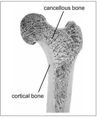
At a macroscopic level, the bone can be divided into compact or cortical and cancellous or trabecular bone. The cortical bone is mostly solid, with only around 10% porosity; on the counterpart, the cancellous bone is formed by an architecture of trabeculae that results in around 50 – 90% porosity with large spaces that are observable at the naked eye (Sikavitsas, et al. 2001, Currey 2002). In the femur, only cortical bone can be identified at the central portion (diaphysis), whereas the extremities (metaphysis) are composed by both types of bone, being the cancellous predominant (Figure 1.3).
Figure 1.3 Cortical and cancellous bone Taken from Willems et al. (2014)
Each type of bone has well differentiated mechanical properties, and these are commonly related to its density (or porosity), allowing for the use of general expressions for the mechanical properties and for the personalization of the finite element (FE) models by relating the density to computer tomography data (see for instance Keyak and Falkinstein (2003), Chanda, et al. (2015)). Moreover, the changes in the bone are often referred to as changes in density (García, et al. 2002, Huiskes, et al. 1987). Therefore, one can also track the evolution of mechanical properties of bone. It is not the objective of this section to provide a detailed review of the reported values for the mechanical properties. Instead, the
aim is to provide the reader with an idea of the ranges for these mechanical properties that allows positioning the bone with respect to other materials. In the following the main mechanical properties of bone and their relationship with bone density (ρ) are depicted.
1.1.3.1 Elastic modulus
The elastic modulus (E) of cortical bone is commonly found in the range 10 GPa – 22 GPa; while for cancellous bone reported values are commonly in the range 0.03 GPa to 2.5 GPa (Reimeringer and Nuño 2014). One of the most commonly used expressions for relating the cortical and cancellous E elastic to ρ (Eq. (1.1)) was proposed by Carter and Hayes (1977).
= 3790 ∙ (1.1)
1.1.3.2 Strength
Similar to the elastic modulus, large variations are found for the strength of bone (Sbone). The
cortical bone strength is commonly reported in the range 133 MPa to 158 MPa (Currey 2002), while the strength of cancellous bone is between 1 MPa and 50 MPa (Carter and Hayes 1977). One of the most common relationships between Sbone and ρ, proposed by
(Carter and Hayes 1977), is shown in (Eq. (1.2)).
= 68 ∙ (1.2)
1.1.3.3 Interfacial strength
At the bone-implant interface, a multiaxial stress state can be identified: normal (traction and compression) and tangential (shear) stresses occur. Stone et al. (1983) and Kaplan et al. (1985) determined the strength of the bone at the interface in both directions, obtaining the power expressions (Eqs. (1.3) - (1.5)) for the traction (St =2.6-7.6 MPa), compression (Sc
= 14.5 1.71 (1.3)
= 32.4 1.85 (1.4)
= 21.6 1.65 (1.5)
1.2 Total hip arthroplasty
Osteoarthritis (OA) or degenerative arthritis is the most common disease of the hip, and consists in the degeneration of the articular cartilage. In advanced stages, it is accompanied by severe pain and limitation in daily activities, and the solution is to perform a total hip arthroplasty (THA) (Siopack and Jergesen 1995, Pivec, et al. 2013). During the period 2013-2014 OA accounted for 74.7% of the hip arthroplasties in Canada while hip fracture was the second most common cause with 14.5% of the replacements (Canadian Institute for Health Information 2015). OA is also the main indication in other countries. For instance, it accounts for 85% of male and 79.8% of female arthroplasties in Sweden (Swedish Hip Arthroplasty Register 2013) and 93% of the replacements in the United Kingdom (UK National Joint Registry 2015).
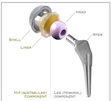
In THA, both sides of the hip joint are replaced with the objective of reducing or eliminating pain and restoring the function of the hip (Pivec, et al. 2013). The most common configuration of hip implants is shown in Figure 1.4. It comprises a metallic shell and a polyethylene or ceramic liner on the acetabular side, and a metallic stem with a metallic or ceramic head on the femoral side. Most modern prostheses allow some degree of modularity, with different choices for the stem neck and head in order to reproduce the adequate anatomy of a healthy hip. This thesis is focused in the femoral component, and in the following the terms (hip) implant or prosthesis will refer to this component
Figure 1.4 Total hip replacement components. Taken from Ever Smith (2007-2008)
Hip stems are usually made of titanium (Ti6Al4V), which has shown superior biocompatibility, corrosion resistance and closer mechanical properties to bone (E=110 GPa), compared to other alloys, such as cobalt-chrome-molybdenum (CoCrMo, E=210 GPa) (Learmonth, et al. 2007, Mai, et al. 2010).
The implant can be fixed using cement (Poly-Methyl Methacrylate Acid), guaranteeing its stability immediately after the operation; however, cementless fixation is preferred nowadays (Berry and Bozic 2010, Pivec, et al. 2013). For this type of fixation, the initial mechanical stability is usually achieved by press-fit (Khanuja, et al. 2011), and the secondary (i.e. long-term) stability is obtained by bone ingrowth (Learmonth, et al. 2007, Mai, et al. 2010). To this end, the implant is made porous where bone ingrowth is desired, and in some occasions, hydroxyapatite (calcium phosphate) is included to enhance osteoconductivity (Learmonth, et al. 2007, Mai, et al. 2010, Khanuja, et al. 2011).
Different stem designs exist with the objectives of establishing proper contact and achieving sufficient initial stability so that bone ingrowth can happen (Khanuja, et al. 2011), and guaranteeing the long-term survivorship of the implant. According to their shape, stem
designs can be classified into: anatomic (Figure 1.5 – a), which try to replicate the natural curvature of the femur; cylindrical (Figure 1.5 – b), which rely on distal cortical support to reach immediate stabilization; and tapered (Figure 1.5 – c), which show a wedged shape and achieve fixation in the cortical bone just below the lesser trochanter (Learmonth, et al. 2007, Mai, et al. 2010). Amongst these designs, anatomic and tapered stems show somewhat better results, compared to cylindrical stems (Mai, et al. 2010) and thus are the most common choice.
a b c
Figure 1.5 (a) Anatomical, (b) cylindrical and (c) tapered cementless stems. The hatched represents the porous coated zone for bone ingrowth.
Adapted from Khanuja et al. (2011)
1.2.1 Epidemiology and future perspectives
In Canada, 49,503 hospitalizations related to hip replacement were registered in the period 2013-2014, which represents an annual increase of 5% and a 5-year increase of 19.1% (Canadian Institute for Health Information 2015). Worldwide the same tendency has been observed, with more than a million THA performed every year and the prevision of doubling this number within the next two decades (Pivec, et al. 2013).
In addition, patients are younger: in Canada, 40.4% (males) and 26.8% (females) of all hip arthroplasties recipients in the period 2013-2014 were under 65 years old (Canadian Institute
for Health Information 2015). In other countries, similar rates have been observed: in Sweden, the proportion of young patients increased from around 50% to almost 60% for men and from around 40% to almost 50% for women in the period 1992-2011 (Swedish Hip Arthroplasty Register 2013). Predictions are that up to 50% of all THA will be done in patients under 65 years old by 2030 (Kurtz, et al. 2009).
1.2.2 Main related problems
The commonly accepted lifespan of a hip stem is 15 years (Siopack and Jergesen 1995); however some studies have found up to 22.6 years implant survivorship (Khanuja, et al. 2011). Multiple factors affect this long-term survivorship of the arthroplasty, including a careful patient selection and surgical technique, the stem design and material resistance (Mai, et al. 2010, Pivec, et al. 2013). Younger patients are considered a risk population for hip arthroplasty, since they have higher activity levels and require implants with increased longevity (Kurtz, et al. 2009). This translates in higher failure rates for younger patients. For instance, in Canada the 5.44% revision rate for patients under 45 years old contrasts with the 1.72% for patients over 85 years old (Canadian Institute for Health Information 2015). In the United Kingdom, patients under 55 years old showed 7.26% 10-year revision rate whereas patients over 75 years old only showed 2.83% (UK National Joint Registry 2015). In Sweden patients under 50 years show up to 40% 20-year revision rate, compared to the 10% for patients over 75 years (Swedish Hip Arthroplasty Register 2013).
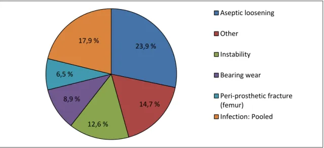
The implant failure comes generally in the form of aseptic (without infection) loosening. This represented 23.9% of failures in Canada in 2015 (Figure 1.6). This is also true worldwide. For instance, aseptic loosening represented approximately 40% of the revisions in Sweden during 2013; and 24.4% of the revisions in the United Kingdom.
Figure 1.6 Causes for revision of the arthroplasty in Canada Source: Canadian Institute for Health Information (2015)
1.3 Numerical analysis of hip implants
In an attempt to improve THA longevity, numerical (finite element) analysis allows researchers to study stresses and strains within the bone and at the stem-bone contact interface, as well as to evaluate implant stability, bone resorption or simulate bone remodeling. Therefore, the causes of mechanical-related implant failure can be analyzed and the implants can be optimized to improve their mechanical compatibility with bone.
1.3.1 Mechanical causes of implant failure
It is believed that the bone loss caused by the stress shielding effect and the interfacial failure due to improper interfacial conditions may contribute to the aseptic loosening of the implant (Kuiper and Huiskes 1997, Arabnejad Khanoki and Pasini 2012).
1.3.1.1 Stress shielding
When the femoral bone is partially replaced by a stiffer metallic hip stem, a redistribution of the mechanical stimuli within the bone occurs in such a way that the stresses are decreased at
23,9 % 14,7 % 12,6 % 8,9 % 6,5 % 17,9 % Aseptic loosening Other Instability Bearing wear Peri-prosthetic fracture (femur) Infection: Pooled
the proximal femur. The bone is hence stress shielded, and being a living tissue that reacts to the mechanical stimuli (Huiskes, Weinans, et al. 1987), bone can be partially resorbed. The clinical impact of such bone resorption due to stress shielding may not be clear yet; however the diminution of the bone stock and quality that this phenomenon causes may compromise a future revision arthroplasty (Kuiper and Huiskes 1992, Mai, et al. 2010). Flexible and less invasive (i.e. smaller) implants have been shown to decrease the stress shielding (Huiskes and Boeklagen 1988, Weinans, et al. 1992, Kuiper and Huiskes 1992). In this way, Kuiper and Huiskes (1992) computed 70% decrease in the resorbed bone mass for a 70% reduction of the implant elastic modulus.
From a computational point of view, the bone resorption due to stress shielding is quantified by means of the changes in the bone density (ρ). Such changes are generally assumed to be proportional to the variations in the strain energy per unit of bone mass (Sen = U / ρ, where U
is the strain energy density). Although detailed algorithms that model the time-dependent ρ evolution exist (see for instance García, et al. (2002)), the simpler formulation proposed by Kuiper and Huiskes (1997) is commonly used for quantifying the effects of stress shielding. This considers that the bone is resorbed if Sen for the implanted bone is lower than a reference
case (Sen,ref), which is usually the original (non-implanted) bone. In order to take into account
the variations in Sen that do not carry changes in ρ, the dead-zone parameter (sd) is
introduced. This formulation gives place to the binary resorption function (g(Sen)) shown in
Eq. (1.6):
( ) = 1 < (1 − ) ∙ ,
0 ℎ (1.6)
and, the resorbed bone mass fraction (mr) can be computed for the entire bone volume (Vbone)
by dividing by the total bone mass (M), as shown in Eq. (1.7).
1.3.1.2 Interfacial failure
Large stresses at the bone-implant contact may result in the interfacial failure. In addition, it has been suggested that they can increase the level of pain and, in the immediate post-operative situation, result in larger interfacial micro-movements that would inhibit bone ingrowth (Kuiper and Huiskes 1997). Similarly to the stress shielding, the interfacial failure depends on the characteristics of the implant (mechanical properties and shape). Kuiper and Huiskes (1992, 1997) showed that the peaks of interfacial stresses are increased and shifted proximally with flexible stems (Figure 1.7), and Chanda et al. (2015) found that less invasive stems would result in more critical interfacial conditions.
a b
Figure 1.7 Interfacial failure index for (a) solid titanium and (b) flexible stems.
Taken from Kuiper and Huiskes (1992)
Few researchers have considered the short-term failure of implants, addressed by the interfacial displacements (Fernandes, et al. 2004, Ruben, et al. 2012). Nevertheless, the most common approach is to consider the long-term failure, based on a local interfacial failure index (fIS) that takes into account normal (σN) and/or shear (τ) interfacial stresses. In its most
general form, this index is based on the Hoffman multiaxial failure criterion (Pal, et al. 2009), as shown in Eq. (1.8).
= + 1 − 1 + (1.8)
The values of St, Sc and Ss are the traction, compression and shear bone interfacial strengths,
which can be related to bone density as shown in section 1.1.3.3. A common simplification to this index is to consider only the failure by shear stress (Kuiper and Huiskes 1997, Arabnejad Khanoki and Pasini 2013b). In such cases, only the last term of Eq. (1.8) is taken into account (fIS = (τ / SS) 2).
A global interface index (FIS) is generally constructed by averaging over the entire area in
contact = 1 ∙ (Kuiper and Huiskes 1997); although formulations based on the maximum local value have also been proposed (Arabnejad Khanoki and Pasini 2013b).
1.3.2 Improvement of stem performance
In the previous section, it was shown that the stem characteristics (e.g. shape and mechanical properties) produce contradictory effects that can lead to implant failure. Therefore a compromise has to been found, and two methodologies to address this specific problem have been proposed: 1) optimize the implant shape and 2) design functionally graded stems.
1.3.2.1 Optimization of implant shape
To optimize the stem shape (Figure 1.8), 2D (Huiskes and Boeklagen 1989, Fernandes, et al. 2004) and 3D (Kowalczyk 2001, Ruben, et al. 2012, Chanda, et al. 2015) models have been employed. In these problems, a set of geometrical variables defines the shape of the stem; while constraint relationships between the variables assure proper shape of the implant. A variety of objective functions have been used based on the interfacial stresses/failure
(Huiskes and Boeklagen 1989, Kowalczyk 2001, Fernandes, et al. 2004, Ruben, et al. 2012), interfacial displacements (Fernandes, et al. 2004, Ruben, et al. 2012), and bone resorption (Ruben, et al. 2012, Chanda, et al. 2015).
Although single-objective optimization has been performed (Kowalczyk 2001), the multi-objective optimization is more common (Fernandes, et al. 2004, Ruben, et al. 2012, Chanda, et al. 2015). In this way, Fernandes et al (2004) compared these two approaches, finding that the multi-objective optimization provides compromise solutions within the boundaries given by the single-objective optimization. For multi-objective optimization, genetic algorithms have been a choice in recent studies (Chanda, et al. 2015) since they allow the determination of a large set of optimal solutions, from which the desired solutions can be selected afterwards according to either one or the other objective.
Figure 1.8 (a) Bone density after remodeling and (b) interfacial failure around a stem with optimized shape.
Adapted from Chanda et al (2015)
In general, stems having wedged shape, with thick distal tip and almost rectangular cross sections improve the primary stability (minimize interfacial displacements) (Fernandes, et al.
2004, Ruben, et al. 2012). On the other hand, minimally invasive implants having small (thin) tip have resulted in decreased interfacial stresses (Fernandes, et al. 2004, Ruben, et al. 2012, Chanda, et al. 2015). Furthermore, such minimally invasive implants lead to a diminution of the bone resorption (Ruben, et al. 2012, Chanda, et al. 2015). Recent studies have shown (Figure 1.8) that optimized stems can reduce the interfacial failure by 68% compared to standard stems, while bone resorption has been decreased from 39% to 24-27% (Chanda, et al. 2015).
1.3.2.2 Functionally graded stems
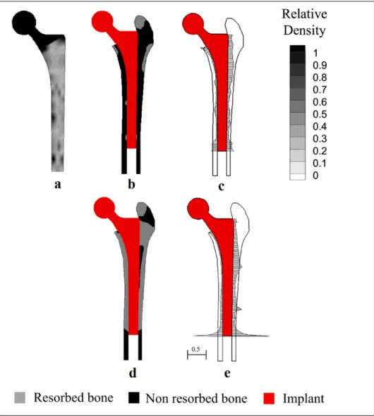
Another approach that has been proposed seeks at optimizing the non-uniform distribution of mechanical properties of the stem (Figure 1.9). Implants conceived according to this principle are said to be functionally graded (FG). For this approach, only 2D models have been considered (Kuiper and Huiskes 1992, Simoes, et al. 1998, Hedia, et al. 2006, Arabnejad Khanoki and Pasini 2012). In this problem, the variables are the mechanical properties (e.g. the elastic modulus) at a certain number of optimization points distributed within the stem. Some authors have evaluated the performance of such stems in terms of a combination of the strain energy density and principal stresses on the bone and the cement (for cemented prostheses) (Simoes, et al. 1998), or a combination of the von Mises stress and the interfacial stresses (Hedia, et al. 2006). However, the most commonly used approach considers the multi-objective optimization in terms of the resorbed bone mass fraction and the interfacial failure (Kuiper and Huiskes 1992, Arabnejad Khanoki and Pasini 2012, 2013b, 2013c).
Figure 1.9 (a) Porous material density distribution; (b) bone resorption; (c) interfacial shear stresses for a functionally graded hip stem; (d) bone resorption; (e) interfacial shear stresses for a solid Ti6Al4V stem.
Adapted from Arabnejad Khanoki and Pasini (2013c)
Different strategies have been proposed for designing the FG of the implants. Kuiper and Huiskes (1992) considered linear variations of the elastic modulus along the stem length. Hedia et al. (2006) performed a linear interpolation between 3 points located at the proximal and distal ends of the FG implant. Simões et al. (1998) compared linear, square root and logarithmic continuous variations of the material of the stem from proximal to distal. More recently, Arabnejad Khanoki and Pasini (2012, 2013b, 2013c) considered a grid of 130 material optimization points uniformly distributed along the stem with linear interpolation
between the points, which resulted in more general non-uniform distribution of the mechanical properties of the stem (Figure 1.9).
In general, best results have been obtained with optimized stems being stiffer at the proximal and medial levels than distally and laterally (Kuiper and Huiskes 1992, Simões, et al. 1998, Hedia, et al. 2006, Arabnejad Khanoki and Pasini 2012). Compared to standard stems, FG stems have shown to reduce stress shielding and yield better interfacial conditions. Arabnejad Khanoki and Pasini (2012) determined that compared to a standard titanium stem, the FG stem could produce 76% and 50% reduction in terms of bone resorption and peak interfacial failure, respectively.
To obtain the FG of material properties, different options have been proposed. Simões et al. (1998) considered a cobalt-chrome core with a controlled stiffness composite outer layer. Hedia et al. (2006) obtained the FG by means of a mixture of collagen, ceramic (bioglass) and metallic materials. Nevertheless, the most interesting approach has been recently proposed by Arabnejad Khanoki and Pasini (2012), who took advantage of additively manufactured porous materials. As it will be described in the next section, such materials allow for the tailoring of their mechanical properties by controlling their geometrical parameters. This has led to an increasing interest for such materials not only for hip stems, but also for other implants where tailored mechanical properties are needed and/or bone ingrowth is desired such as long bone default regeneration (Wieding, et al. 2014), acetabular cups with enhanced fixation properties (Marin, et al. 2010), or stems for total knee arthroplasty with better mechanical compatibility with the bone (Murr, et al. 2011).
1.4 Porous materials
Gibson and Ashby (1999) defined a porous material as “an interconnected network of solid struts or plates which form the edges and faces of cells”. Since such network has its own set of effective mechanical properties, it is a material itself and can be compared with common bulk materials (Ashby, 2006). The material can be found forming walls (or plates), resulting
in “closed-cell” porosity; or struts, resulting in an interconnected network of “open-cell” pores (Gibson 2005). On the other hand, the porous material may have a random nature, in which case it is referred to as foam; or result from the 3D uniform repetition of a base unit cell (tessellation), in which case it is called lattice or well-ordered.
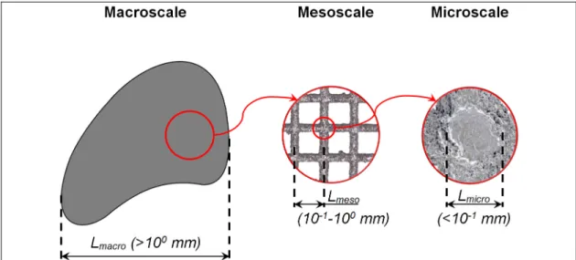
Three different size levels or scales can be identified in a porous material: macroscale, mesoscale and microscale (Figure 1.10). The macroscale defines the (external) dimensions of the part, and it can go from some millimeters to several centimeters. At the mesoscale, the details of the porous structure can be observed (e.g. unit cell shape and dimensions). This scale goes from hundreds to some thousands of microns, lying between the macroscale and the microscale. The microscale which cannot be seen to the naked eye, goes up to several micrometers and contains information at the strut level (e.g. crystallographic composition of the material).
Figure 1.10 Macroscale, mesoscale and microscale of a porous material
1.4.1 Well-ordered porous materials
Non stochastic (i.e. well-ordered) porous materials result in similar stiffness than stochastic foams (Murr, et al. 2011), with higher specific strength (Cheng, et al. 2012). Therefore, this thesis is focused on porous materials having a well-ordered structure at the mesoscale
(lattices). Furthermore, since the planned application is load-bearing prosthesis, titanium (Ti6Al4V) material is considered for being the most commonly used material in hip stems (Learmonth, et al. 2007, Mai, et al. 2010). In the following, the terms porous, lattice, well-ordered porous or cellular materials may be used indistinctively, referring in all cases to porous materials resulting from the 3D repetition of a base unit cell.
1.4.2 Main geometrical parameters of porous materials
The unit cell geometry at the mesoscale plays an important role not only on the structural dimensions, but also on the mechanical behavior of porous materials (Gibson 2005). Amongst the different unit cell geometries that have been considered in experimental or computational studies, the two most common are the simple cubic (Heinl, et al. 2008, Parthasarathy, et al. 2010, Parthasarathy, et al. 2011, Hazlehurst, et al. 2013) and diamond unit cells (Cansizoglu, et al. 2008, Heinl, et al. 2008, 2008b, Marin, et al. 2010, Hrabe, et al. 2011, Ahmadi, et al. 2014, Herrera, et al. 2014, Horn, et al. 2014). These are shown in Figure 1.11.
a b
Figure 1.11 (a) Simple cubic and (b) diamond unit cells
Even though porous materials have such non-homogeneous structure at the mesoscale, they are treated as homogeneous at the macroscopic level. Macroscopic dimensions (and mechanical properties) are thus said to be apparent, and they are the dimensions (and mechanical properties) as of the “equivalent” fully solid material. These dimensions can be
computed as the product of the unit cell length at the mesoscale (LUC) times the number of
unit cells (np) in each spatial direction. The unit cell length depends on the geometry of the
unit cell and on the strut (ϕS) diameter and pore (ϕP) diameter (i.e. the diameter of the largest
sphere that can be inscribed in the pore or its 2D projection).
Other parameters, that can be derived from the fundamental ones (LUC, ϕS, and ϕP), are used
for relating the mechanical behavior to the structure of porous materials: the relative density (ρr), defined as the ratio from the apparent density of the porous material (ρapp) to the density
of the solid material (ρs) (Gibson, 2005); the porosity (P%), which is equivalent to ρr (Eq.(1.9)
) and defined as the ratio of the volume of the pores (Vpores) to the apparent volume of the
porous material (Vapp) (Parthasarathy, et al. 2011); or the slenderness ratio (SR), which gives
an idea of the length-to-thickness of the struts (see section 3.3.1).
= = =
∙
= = 1 − = 1 − %
100
(1.9)
where ms is the mass of the porous material, Vsolid is the volume of the solid part of the porous
material.
1.4.3 Additive manufacturing of porous materials
The production of materials having such complex, well-controlled porous mesostructure is possible thanks to additive manufacturing technologies (Murr, et al. 2012). In particular, powder-beam based technologies, such as Electron Beam Melting (EBM) and Selective Laser Melting (SLM), also known as Direct Metal Laser Sintering (DMLS) are very popular for the production of such materials.
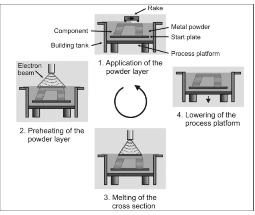
Figure 1.12 The process of additive manufacturing. Taken from (Heinl, et al. 2008)
Both EBM and SLM (or DMLS) share the same working principle (Figure 1.12). The CAD model of the part to be produced is first sliced in a number of cross-sections. Then an iterative process begins, where the material powder is extended in the fabrication platform. A beam preheats the powder bed and then selectively melts the zones that conforms a specific cross-section of the part. Afterwards the fabrication platform is lowered, a new powder layer is extended and the process is repeated until the part is completed (Heinl, et al. 2008).
The main differences between EBM and SLM processes are outlined in Table 1.2. Apart from differences concerning the powder size, layer thickness and building rate, the most relevant discrepancies arise from the nature of the beam (electron or laser), which forces the EBM technology to work with conductive materials, and also from the working environment that for EBM is vacuum while for DMLS is a mix of inert gas.
Table 1.2 Differences between EBM and DSLM technologies
EBM SLM/DMLS
Beam Nature Electron Laser
Min. Diameter (µm) 100 a) 100 e)
Powder size (µm) 45 – 100 b) 5 – 50 f)
Accuracy (µm) 130 c) ± 50 (wall thickness 0.3
– 0.4 mm) f)
Layer thickness (µm) 100 d) 20 – 100 e)
Building rate (mm/h) 6 – 7 d) (55-80 cm3/h c)) 7 – 8 d) (7.2-72 cm3/h e))
Environment Vacuum (10pressure of He (10-5 bar) / Partial -3 bar) a) Argon/nitrogen mix d)
Other Conductive materials.
Pre-sintering of the powder
Note: a) (ARCAM AB, Q10 brochure), b) (ARCAM AB, Ti6Al4V ELI Titanium Alloy brochure), c) (ARCAM AB, A1 brochure), d) (Koike, et al. 2011), e): (EOS, EOSINT M270 brochure), f) (Rehme and Emmelmann 2006), g) (EOS, Titanium Ti64ELI brochure)
1.4.3.1 Irregularities of additively manufactured porous materials
EBM and SLM/DMLS are considered to allow the manufacturing of porous materials with high degree of control over the dimensions at the mesoscale; however, differences between designed and manufactured dimensions arise (Harrysson, et al. 2008). Since the mesoscale dimensions of the porous materials are typically of the same order of magnitude of the accuracy of the technologies (hundreds of microns), the manufacturing errors can represent large percentages of the design dimensions.
At the macroscale, the manufactured sample size of EBM-produced porous materials has been found to be 1% larger than the designed size, with porosity variations up to 23.5% (Parthasarathy, et al. 2011).