Cross–Sectoral Variation in Firm–Level
Idiosyncratic Risk
∗Rui Castro† Gian Luca Clementi‡ Yoonsoo Lee§
This version: October 12, 2010 [Link to the latest version]
Abstract
We estimate firm–level idiosyncratic risk in the U.S. manufacturing sector. Our proxy for risk is the volatility of the portion of growth in sales or TFP which is not explained by either industry– or economy–wide factors, or firm characteris-tics systematically associated with growth itself. We find that idiosyncratic risk accounts for about 90% of the overall uncertainty faced by firms. The extent of cross–sectoral variation in idiosyncratic risk is remarkable. Firms in the most volatile sector are subject to at least three times as much uncertainty as firms in the least volatile. Our evidence indicates that idiosyncratic risk is higher in industries where the extent of creative destruction is likely to be greater.
Key words: Schumpeterian Competition, Creative Destruction, Product Turnover, R&D Intensity, Investment–Specific Technological Change.
JEL Codes: D24, L16, L60, O30, O31.
∗We are grateful to Mark Bils, Yongsung Chang, Massimiliano Guerini, and Roberto Serrano
for very helpful comments. A special thank goes to Gianluca Violante and Jason Cummins for providing us with their data on investment–specific technological change, and to Yongsung Chang and Jay Hong for supplying us with their ELI–SIC correspondence table. The views expressed in this article are those of the authors and do not necessarily reflect the position of the Federal Reserve Bank of Cleveland or the Federal Reserve System. The research in this paper was conducted while Yoonsoo Lee was a Special Sworn Status researcher of the U.S. Census Bureau at the Michigan Census Research Data Center. Research results and conclusions expressed are those of the authors and do not necessarily reflect the views of the Census Bureau. This paper has been screened to insure that no confidential data are revealed. Support for this research at the Michigan RDC from NSF (awards no. SES–0004322 and ITR–0427889) is gratefully acknowledged. Castro acknowledges financial support from SSHRC.
†Department of Economics and CIREQ, Universit´e de Montr´eal. Email:
[email protected]. Web:https://www.webdepot.umontreal.ca/Usagers/castroru/MonDepotPublic
‡Department of Economics, Stern School of Business, New York University andRCEA. Email:
[email protected]. Web: http://pages.stern.nyu.edu/˜gclement
§Department of Economics, Sogang University and Federal Reserve Bank of Cleveland. Email:
1
Introduction
The main goal of this study is to assess the cross–sectoral variation in firm–level idiosyncratic risk in U.S. manufacturing. Our data consists of a large panel extracted from the U.S. Census’ Longitudinal Research Database (LRD).
We proxy idiosyncratic risk with the portion of the variation in growth (in sales or TFP) that is not accounted for by aggregate disturbances or by other factors that vary systematically with growth, such as age and size.
Our manufacturing–wide estimates suggest that idiosyncratic risk is substantially larger than aggregate risk. The volatility of annual sales growth is about 10%, while the volatility of TFP growth is roughly 8%. As a term of comparison, notice that between WWII and the great moderation the standard deviation of U.S. annual real GDP growth was only 2.52%.
The variation in idiosyncratic risk across three–digit industries is substantial. To gain a flavor of the amount of heterogeneity we uncover, consider that the volatility of sales growth ranges from 3.78% for publishers of newspapers to a whopping 18.53% for manufacturers of railroad equipment.
Why does volatility differ so much across sectors? We provide some preliminary evidence in favor of a particular explanation: volatility is higher in sectors where creative destruction is more important.
The notion of creative destruction is central to the Schumpeterian paradigm. Ac-cording to the latter, firms are engaged in a perpetual race to innovate. Creation, i.e. the success by a laggard in implementing a new process or producing a new good, displaces the previous market leader, eliminating (destroying) its rent.
Formal models of Schumpeterian competition1
predict a positive cross–sectoral association between creative destruction, product turnover, and innovation–related activities. We document that idiosyncratic risk is higher in industries where product turnover is greater and investment–specific technological progress is faster.
Learning about the magnitude of firm–level idiosyncratic risk is important in light of the remarkable role that the latter plays in many areas of applied economics. In
Hopenhayn(1992) andEricson and Pakes(1995), two of the most popular frameworks
for the study of industry dynamics, as well as in theories of financing constraints based on asymmetric information, such as Clementi and Hopenhayn (2006) and Quadrini
(2003), firms are modeled as risk–neutral agents facing sequences of idiosyncratic 1
shocks.
Given that firms’ stakeholders have often limited insurance opportunities, assess-ing firm–level risk is also relevant for the analysis of scenarios where risk aversion matters. This is the case of entrepreneurship studies such as Quadrini(1999), theo-ries of economic development such asCastro, Clementi, and MacDonald (2004,2009), and models of innovation such as Caggese (2008).
The evidence of lack of diversification abounds. Clementi and Cooley (2009) document that in 2006, more than 20% of CEOs of U.S. publicly–traded concerns2
held more than 1% of their companies’ common stock. About 10% held more than 5%. Given the large capitalization of such companies, this information points to limited portfolio diversification for these individuals. Herranz, Krasa, and Villamil (2009) find that 2% of the primary owners of the firms sampled by the 1998 Survey of Small Business Finance3
invested more than 80% of their personal net worth in their firms; 8% invested more than 60%, and about 20% invested more than 40%.
We are not the first to realize the need of assessing risk at the firm level. Campbell,
Lettau, Malkiel, and Xu(2001) proxied risk with the volatility of excess stock returns.
They decomposed the latter in three components: aggregate, industry–wide, and firm–level. This allowed them to obtain average measures of idiosyncratic risk for the whole economy and for several coarsely defined sectors.
Our view is that their methodology delivers reasonable proxies for the risk borne by equity investors, but not for that faced by other stakeholders, such as the owners of small firms. This is the case for three reasons. First of all, COMPUSTAT only includes publicly traded companies, and therefore is not representative of the universe of firms in the U.S. Second, their measure of firm–level volatility clearly depends on the volatility of the stochastic discount factor and on the covariance of the latter with cash flows. Finally, the cash flows are those expected to accrue to equity investors. This implies, for example, that they are affected by leverage.
Our exercise is closer to those carried out in more recent papers, that exploit bal-ance sheet information rather than stock market data. We refer to the contributions
of Abraham and White (2006), Bachman and Bayer (2009), andGourio (2008), who
estimate processes for idiosyncratic risk using unbalanced panels from the U.S. Cen-2
The data is from EXECUCOMP, a proprietary database maintained by Standard & Poor’s that contains information about compensation of up to 9 executives of all companies quoted in organized exchanges in the U.S.
3
The SSBF, administered by the Board of Governors of the Federal Reserve System, surveys a large cross–sectional sample of non–farm, non–financial, non–real estate firms with less than 500 employees.
sus’ LBD, Deutsche Bundesbank’s USTAN, and Compustat, respectively. We also think of the work by Comin and Mulani (2006), Comin and Philippon (2005), and
Davis, Haltiwanger, Jarmin, and Miranda (2006).
Our study is different from all the above, in that it illustrates the cross–sectoral variation in firm–level idiosyncratic uncertainty. We provide estimates of risk by three–digit SIC sectors and make a first attempt at identifying the determinants of the heterogeneity we uncover.
Understanding how idiosyncratic risk varies across industries is a necessary step towards the quantitative evaluation of a recent breed of multi–sector models, such
asCastro, Clementi, and MacDonald (2009), Cu˜nat and Melitz (2010), and Caggese
(2008). According to the first two, cross–sectoral differences in idiosyncratic risk, together with cross–country heterogeneity in institutions, rationalize the observed cross–country variation in relative price of capital goods and investment rate (the former), and trade specialization (the latter). Caggese (2008) studies the impact of idiosyncratic risk on entrepreneurial firms’ propensity to innovate.
To our knowledge, four other studies set out to characterize the extent of cross– sectoral variation in firm–level volatility. Michelacci and Schivardi (2008) use a methodology close to Campbell, Lettau, Malkiel, and Xu (2001). Castro, Clementi,
and MacDonald (2009) and Cu˜nat and Melitz (2010) estimate the volatility of sales
growth in COMPUSTAT. Chun, Kim, Mork, and Yeung (2008) find that, for COM-PUSTAT firms, the heterogeneity of firm–specific stock returns and sales growth is higher in 2–digit SIC sectors that use information technology more intensively.
The gain from using the LRD in place of COMPUSTAT is substantial. To start with, the LRD is a much larger sample. This allows us to work with a finer sector classification. Furthermore, the sampling technique ensures that the LRD is repre-sentative of the population of manufacturing firms. Since COMPUSTAT only covers companies whose stock is traded in an organized exchange, it is severely biased to-wards large firms.
Finally, the better quality of the data on investment allows us to compute reliable estimates of TFP growth. The conditional volatility of sales growth is not the ideal proxy for idiosyncratic risk because swings in a firm’s sales depend not only on the shocks, which size we are interested in measuring, but also on the firm’s ability to alter its inputs to accommodate them. The volatility in firm–level TFP growth is exempt from this criticism.
are described in Section 2. Our volatility estimates across three–digit industries are illustrated in Sections 3. In Section 4 we illustrate evidence in support of the con-jecture that idiosyncratic risk is greater in industries where creative destruction is more important. In Section 5 we show that, consistent with what found by Castro,
Clementi, and MacDonald (2009) for public firms, firms that produce capital goods
are systematically riskier than their counterparts producing consumption goods. Fi-nally, Section 6 concludes.
2
Data and Methodology
2.1 Data
Our data is from the Annual Survey of Manufactures (ASM) portion of the Longi-tudinal Research Database (LRD) for the years 1972 through 1997. Depending on the year, its size varies from 50,000 to 70,000 establishments, distributed among 140 three–digit SIC manufacturing industries. With the ASM weights, our sample ends up being representative of the entire U.S. manufacturing sector.
Our unit of observation is the establishment, defined as the minimal unit where production takes place. This is obviously short of ideal, as multi–plants firms may change the assignment of production to manufacturing units in response to shocks. In the remainder, we will use the terms plant and firm interchangeably.
Using the LRD rather than COMPUSTAT has a variety of advantages. To start with, our results are not subject to the selection bias emphasized by Davis,
Halti-wanger, Jarmin, and Miranda (2006), who document a behavior of public firms
markedly different from that of private firms, absent in COMPUSTAT. Furthermore, the LRD allows for a finer level of disaggregation. Our analysis is at the three– digit SIC sectoral level, which maps into four– and five–digit NAICS. Working with COMPUSTAT, Castro, Clementi, and MacDonald (2009) could not go finer than three–digit NAICS. Finally, the LRD allows us to compute reliable estimates of firms’ capital stocks, which is necessary to compute Solow residuals.
For our purposes, the only drawback of the LRD is that it only covers manufac-turing firms, whereas COMPUSTAT spans all sectors.4
Real sales are the nominal value of shipments, deflated using the four–digit industry– specific deflator from the NBER manufacturing productivity database. Size is mea-sured by the number of employees, whereas age is the time since the establishment
4
The Census Bureau’s Longitudinal Business Database (LBD) has a broader coverage. However, since it does not contain information on capital stocks, it is not suited to computing firm–level TFP.
went into operation.5
Following Foster, Haltiwanger, and Krizan (2001), Baily, Hulten, and Campbell
(1992), andSyverson(2004), we define TFP levels as firm–level Solow residuals. The (log) Solow residual for firm i in sector j at time t is
ln zijt= ln yijt−αkj ln kijt−αℓjln ℓijt−αmj ln mijt,
where yijtis shipments, kijt is capital, ℓijtis labor, and mijtis materials. The
elastic-ities αk
j, αℓj and αmj are assumed to be sector–specific. As in the literature just cited,
we set them equal to narrowly–defined sectoral input cost shares. For further details, see Appendix A.1.
Notice that changes in our measures of real sales and TFP reflect not only fluc-tuations in quantities, but also within–industry price variation. Our TFP measure is what has become known in the literature as real revenue per unit input, or TFPR. This definition is perfectly suited for our study, as we are interested in identifying all sources of idiosyncratic uncertainty, including price variation.
2.2 Methodology
The methodology is going to be the same for either measure of firm growth, based on either sales or TFP. For convenience, we describe it in the case of sales. First, we estimate
∆ ln(sales)ijt = µi+ δjt+ β1jln(size)ijt+ β2jAgeijt+ εijt. (1)
The dependent variable is the growth rate of real sales for firm i in sector j, between years t and t + 1. The dummy variable µi is a firm–specific fixed effect that accounts
for unobserved persistent heterogeneity across firms. The variable δjt denotes a full
set of sector–specific year dummies, which control for changes in sales induced by sector–specific shocks and cross–sectoral differences in business cycle volatility. We include size and age because both were shown to be negatively correlated with firm growth.6
Regression (1) computes the systematic, or predictable component of sales growth. Any variation in sales growth not due to systematic factors is captured by the esti-mated residuals ˆεijt. These are the objects of interest, since they are interpreted as
realizations of firm–specific shocks. 5
In our regression analysis, we follow Davis, Haltiwanger, and Schuh (1996) in that we use 3 categories of age dummies: Young, Middle-Aged, and Mature.
6
The second step consists in measuring how the standard deviation of such shocks varies across sectors. This is accomplished by fitting a simple log–linear model to the variance of residual sales growth:
ln ˆε2
ijt= θj+ vijt, (2)
where θj is a sector–specific dummy variable. Letting ˆθj denote its point estimate,
q
exp(ˆθj) is our measure of the conditional standard deviation of sales growth for
firms in sector j.
3
Volatility Estimates
The mean standard deviation of annual sales growth across all manufacturing plants is 10.07%. As expected, the standard deviation of TFP growth is lower, at 8.05%. The reason is that changes in sales accompanied by changes in inputs in the same direction result in smaller changes in TFP (in absolute value).
Our estimates suggest that idiosyncratic risk is substantially larger than aggregate risk. This can be appreciated by comparing them with readily available measures of aggregate volatility. The average standard deviation of U.S. annual real GDP growth was 2.52% before the great moderation (i.e. in the period 1950–1978) and fell to 1.75% in the period 1979–2007.
A more formal way of assessing the importance of idiosyncratic risk Vs. aggre-gate risk is to compare the former with more comprehensive measures of firm–level uncertainty, which also reflect the portion that may be ascribed to industry–wide and economy–wide factors. Such measures can be calculated by regressing log–sales (or log–TFP) on firm fixed effects only and computing the standard deviation of the residuals.
This exercise yields volatility estimates that are only marginally greater than our measures of idiosyncratic risk. The overall volatility of sales growth is estimated to be 11.58%. That of TFP growth is 9.45%. Idiosyncratic factors appear to account for about 90% of overall firm–level uncertainty.
Our volatility estimates across three–digit industries are reported in Table5 and illustrated in Figure1. The height of each bin is the fraction of sector whose estimated risk falls in the associated interval.
The range of estimates is rather wide, no matter the proxy. The volatility of sales growth is as low as 3.78% for Newspaper Publishing (SIC 271) and as high as 18.53% for Railroad Equipment (374). The volatility of TFP growth is lowest in the Fur
0 .05 .1 .15 .2 .25 Fraction .04 .07 .1 .13 .16 .19 Volatility in sales growth
0 .05 .1 .15 .2 .25 Fraction .04 .07 .1 .13 .16 .19 Volatility in TFP growth
Figure 1: Histogram of idiosyncratic risk by sector.
Goods sector (237), at 4.09%, and highest in Computer Equipment Manufacturing (357), at 12.39%.
The orderings delivered by the two measures are fairly consistent. The Spearman’s rank–correlation coefficient is 0.71.
Drawing comparisons between our estimates of sales growth volatility and those recovered byCastro, Clementi, and MacDonald(2009) (CCM from now on) for public companies is interesting, but is subject to a couple of important caveats. First and foremost, our data is at the plant–level, while theirs is at the firm level. Secondly, their sector classification is at the three–digit NAICS, which is coarser than ours.
For the sectors for which a match is possible, our estimates are sensibly higher. For Computer and Electronic Product Manufacturing, CCM report an estimate of 10.52%, lower than the 15.87% we estimate for SIC 357. For Machine Manufacturing, they estimate volatility at 8.89%, a figure lower than our estimates for all sectors producing machinery (SIC 352, 354, 355, 356, and 358). Similarly, their 4.9% estimate for Food Manufacturing is lower than our estimates for the three–digit SIC sectors that belong to that industry (SIC 201 through 207 plus 209).
This pattern is consistent with the findings of Davis, Haltiwanger, Jarmin, and
Miranda (2006), who compare the volatility of public Vs. privately held firms, and
with the industrial organization literature that documents the negative correlation between growth volatility and size.
4
Creative Destruction and Volatility
Why does volatility differ so much across sectors? In this section, we look for evidence in favor of a particular explanation: volatility is higher in sectors where the speed and extent of creative destruction are greater.
Joseph Schumpeter envisioned economic progress as the result of a perpetual race between innovators. Success by a laggard or an outsider in implementing a new process or producing a new good, provides them with a competitive advantage and displaces the previous market leader, eliminating its rent. This, in a nutshell, is the process of creative destruction.
We conjecture that most of the firm–level volatility that we document reflects the turnover between market participants which is at the center of Schumpeter’s paradigm. That is, we argue that a large fraction of the fluctuations in a firm’ sales and TFP growth is due to variations in its distance from the technology frontier.
Our strategy consists in looking for sector–specific attributes that are likely to be systematically associated with the speed of turnover. Starting with Aghion and
Howitt (1992), Schumpeter’s idea was formalized in a large number of models. We
turn to this literature for guidance.
In Aghion and Howitt (1992), the producer endowed with the leading
technol-ogy monopolizes the intermediate good market. Technoltechnol-ogy improves as a result of purposeful research and development, which in equilibrium is only carried out by prospective entrants. When it succeeds in obtaining a new and more productive vari-ety of intermediate good, the innovator enters and displaces the monopolist. It follows that all the variation in sales growth is associated with product turnover.
The positive association between product turnover and firm–level volatility is not specific to Aghion and Howitt (1992). Rather, it is a robust feature of all of its generalizations in which intermediate goods of different vintages are vertically differ-entiated. For example, see Aghion, Harris, Howitt, and Vickers (2001) and Aghion,
Bloom, Bludell, Griffith, and Howitt (2005).
components which embed innovations made by others. This is the scenario described
by Copeland and Shapiro(2010), who model the personal computers industry. The
adoption decision, which entails the introduction of a new product, leads to a rise in sales for the adopter, and to a decline for its competitors.
In Samaniego (2009), the decision that yields a competitive advantage is that of
acquiring the latest vintage of equipment. The faster is investment–specific techno-logical change, the more frequent is technology adoption by either laggards or new entrants. In turn, this leads to a more frequent turnover in industry leadership and more variability in sales growth.
In the next section, we ask whether product turnover is indeed higher in industries where firms are documented to face a greater volatility of sales and TFP growth. In Sections4.2and4.3we will ask whether our volatility measures are positively related with the intensity of R&D and the speed of investment–specific technological change, respectively.
4.1 Product Turnover
The U.S. Bureau of Labor Statistics collects prices on 70,000–80,000 non–housing goods and services from around 22,000 outlets across various locations. When a product is discontinued, the agency starts collecting prices of a closely related good at the same outlet, and records the substitution information. The BLS classifies goods in narrowly–defined categories known as entry–level items (ELI).
Our proxy for turnover is the average monthly frequency of substitutions, known as the item substitution rate. It is the fraction of goods in the ELI that are replaced on average every month. Our data is drawn from Bils and Klenow (2004)’s tabulations, which in turn are based on information on more than 300 consumer good categories from 1995 to 1997.7
Using the algorithm developed byChang and Hong(2006), we were able to match 53 three–digit SIC manufacturing sectors with at least one ELI. For 21 sectors, the correspondence is one–to–one. The remaining 32 are matched to 213 items. In such cases, we defined the substitution rate as the average of the associated ELIs’ rates, weighted by their respective CPI weights.
7
The BLS distinguishes between two types of substitutions. Substitutions are comparable when the replacement does not represent a quality improvement over the previous item. They are non-comparable, otherwise. Since average and noncomparable average item substitution rates are highly correlated across good categories, our results did not change much when we used noncomparable item substitution rates instead.
Two caveats are worth mentioning. To start with, the BLS data focuses on con-sumer goods. Most investment good sectors are missing. Furthermore, the substitu-tion rate only tells about the “frequency” of product turnover and does not provide information about the “size of the step”, i.e. the extent to which a new product improves over the pre–existing one.
202 203 204 205 206 207 208 209 225 227 231 232 233 234 236 238 239 243 251 259 267 271 272 273 283 284 285 289 291 295 299 301 308 314 316 322 326 342 343 352 357 358 363 364 365 366 384 385 387 391 393 394 395 .03 .04 .05 .06 .07 .08 .09 .1 .11 .12 .13 .14 .15 .16
Volatility of sales growth
0 5 10 15 20
Average item substitution rate
Raw correlation: 0.54; (excluding 233,236,357): 0.36.
202 203 204 205 206 207 208 209 225 227 231 232 233 234 236 238 239 243 251 259 267 271 272 273 283 284 285 289 291 295 299 301 308 314 316 322 326 342 343 352 357 358 363 364 365 366 384 385 387 391 393 394 395 .03 .04 .05 .06 .07 .08 .09 .1 .11 .12 .13 .14 .15 .16 Volatility of TFP growth 0 5 10 15 20
Average item substitution rate
Raw correlation:0.57; (excluding 233,236,357): 0.23.
Figure 2: Idiosyncratic Risk and Product Substitution Rate.
The scatter plots in Figure2show that our proxy for product turnover is positively associated with both measures of volatility. The simple correlation coefficients are 0.543 and 0.571 in the cases of sales and TFP, respectively.
Three sectors stand out, as they are characterized by high volatility measures and remarkably high substitution rates. They are Computer and Office Equipment (357), Women’s and Misses’ Outerwear (233), and Girls’ and Children’s Outerwear (236). Anecdotal evidence as well as scholarly research8
suggest that SIC 357 epitomizes the idea of creative destruction. However, product turnover in the other two sectors is not likely to be driven by technological improvements.
Idiosyncratic risk and turnover are positively associated even when we exclude 8
SIC 233, 236, and 357. However, the correlation coefficients drop to 0.359 and 0.235, respectively.
The first two columns in Table 1 report the results of regressing sales growth volatility on the average substitution rate and a constant. Column (1) tells us that on average, a 1% higher substitution rate implies a 0.31% higher volatility of sales growth. In column (2) we drop SIC 233, 236, and 357. The coefficient increases slightly, but the R2
is reduced by half.
Table 1: Idiosyncratic Risk and Product Substitution Rate.
Dependent Variable: Sales volatility TFP volatility
(1) (2) (3) (4) Substitution Rate 0.0031∗∗∗ 0.0034∗∗ 0.0025∗∗∗ 0.0016 (0.0007) (0.0013) (0.0005) (0.0009) Constant 0.0870∗∗∗ 0.0862∗∗∗ 0.0666∗∗∗ 0.0697∗∗∗ (0.0038) (0.0052) (0.0028) (0.0039) Observations 53 50 53 50 R2 0.295 0.129 0.326 0.055
Standard errors in parenthesis. ∗∗∗Significant at 1%. ∗∗Significant at 5%. ∗Significant at 10%.
According to the results listed in column (3), on average a 1% higher substitution rate is associated with a 0.25% higher TFP growth volatility. Without SIC 233, 236, and 357 (see column (4)), the R2
is lower. The coefficient is only marginally insignificant at the 10% confidence level (its p–value is 0.101).
Many establishments in the LRD are likely to produce more than one product. Possibly, many more. As long as the correlation between sales from different lines of business is less than 1, plant–level sales growth volatility will be lower than average volatility at the level of product line. This may explain why sectors such as Glass and Glassware (322), Books (273), and Household Furniture (251) are characterized by a relatively high item substitution rate and low volatility of both sales and TFP growth.
4.2 R&D Intensity
Unfortunately we lack data on research and development expenditure in the LRD. We measure a sector’s research intensity as the ratio of R&D expenditure to sales in COMPUSTAT. The latest CENSUS–NSF R&D survey found that most of the research and development activity takes place at large firms. This leads us to think
that the cross–sectoral variation in R&D expenditures in the population is not likely to differ much from that for large, public firms.
The cross–industry variation in research expenditures that we uncover is substan-tial. Our measure of research intensity varies from 0.022% for Book Binding (SIC 278) to 7.77% for firms in Drugs (283).
202 203 204 205 206 207 208 209 221 222 225 227 232 233 234239 242 243 245 251 252 253 254 259 261 262 263 265 267 271 272 273 274 275 276 278 279 281 282 283 284 285 286 287 289 291 295 299 301 302 305 306 308 314 321 322 323 324 325 326 327 329 331 332 333 334 335 336 339 341 342 343 344 345 346 347 348 349 351 352 353 354 355 356 357 358 359 361362 363 364 365 366 367 369 374 375 376 379 381 382 384 385 387 391 393 394 395 396 .03 .04 .05 .06 .07 .08 .09 .1 .11 .12 .13 .14 .15 .16 .17 .18 .19
Volatility of sales growth
0 .02 .04 .06 .08 R&D Intensity 202 203 204 205 206 207 208 209 221 222 225 227 232 233 234 239 242 243 245 251 252 253 254261259 262 263 265 267 271 272 273 274 275 276 278 279 281 282 283 284 285 286 287 289 291 295 299 301 302 305 306 308 314321 322 323 324325 326327 329 331332 333 334 335 336 339 341343342 344 345 346 347 348 349 351 352 353 354 355 356 357 358 359 361362 363 364 365 366 367 369 374 375 376 379 381 382 384 385 387 391 393 394 395 396 .03 .04 .05 .06 .07 .08 .09 .1 .11 .12 .13 .14 .15 .16 .17 .18 .19 Volatility of TFP growth 0 .02 .04 .06 .08 R&D Intensity
Figure 3: Idiosyncratic Risk and R&D.
The unconditional relationship between our risk proxies and research intensity is illustrated in Figure 3. In Table 2 we report the results of regressing the two volatility measures on R&D intensity and a constant. In the case of sales volatility, the coefficients are not statistically significant. In the case of TFP volatility, the coefficient of R&D intensity is statistically and economically significant. At the mean, a 1% increase in research intensity implies an increase in TFP growth volatility of about 30%.
4.3 Investment–Specific Technological Change
In a simple two–sector model where investment and consumption goods are produced competitively, the quality improvement in the investment good equals the negative
Table 2: Idiosyncratic Risk and Research Intensity.
Dependent Variable: Sales volatility TFP volatility
R&D Intensity 0.2033 0.2938∗∗∗ (0.1292) (0.0858) Constant 0.0986∗∗∗ 0.0725∗∗∗ (0.0027) (0.0018) Observations 109 109 R2 0.0226 0.0988
Standard errors in parenthesis. ∗∗∗Significant at 1%. ∗∗Significant at 5%. ∗Significant at 10%.
of the change in its relative price. Exploiting this restriction,Cummins and Violante
(2002) computed time series of quality improvement – or technical change – for a variety or equipment goods over the period 1948–2000.
Using detailed data on capital expenditures by two–digit SIC industries provided by the Bureau of Economic Analysis, Cummins and Violante (2002) also constructed measures of investment–specific technological change by sector. In this section we ask whether such measures are systematically related to our proxies for risk.
20 21 22 23 24 25 26 27 28 29 30 31 32 33 34 35 36 38 39 .05 .06 .07 .08 .09 .1 .11 .12 .13 .14
Volatility of sales growth
.025 .03 .035 .04 .045 .05 Investment−specific technical change
Raw correlation (excluding 27): 0.54
20 21 22 23 24 25 26 27 28 29 30 31 32 33 34 35 36 38 39 .05 .06 .07 .08 .09 .1 .11 .12 .13 .14 Volatility of TFP growth .025 .03 .035 .04 .045 .05 Investment−specific technical change
Raw correlation (excluding 27): 0.49
Figure 4: Idiosyncratic Risk and Investment–Specific Technological Change. Given the level of aggregation in the data on technological change, our analysis is confined to 19 two–digit SIC sectors, listed in Table6. For each industry, the rate of technological change is the average of the 1948–1999 annual time–series underlying Figure 2 inCummins and Violante (2002), provided to us by Gianluca Violante. The risk proxies are weighted averages of the volatility estimates for the three–digit SIC sectors that belong to the industry. The weights are the values of the average share
of each 3-digit sector’s value of shipments in the corresponding two–digit sector.9
The scatter plots in Figure4 suggest a positive association between the two vari-ables. Sectors such as SIC 35 (Industrial and Commercial Machinery and Computer Equipment) and 31 (Leather and Leather Products) display high volatility and high investment–specific technological change. SIC 34 (Fabricated Metal Products, except Machinery and Transportation Equipment), which ranks last in terms of technological change, is also among the least uncertain sectors.
Table 3: Idiosyncratic Risk and Investment–Specific Technological Change.
Dependent Variable: Sales volatility TFP volatility
ISTC 1.1235∗∗ 0.9370∗∗ (0.5174) (0.3767) Constant 0.0997∗∗∗ 0.0417∗∗∗ (0.0627) (0.0141) Observations 18 18 R2 0.228 0.279
Standard errors in parenthesis. ∗∗∗Significant at 1%. ∗∗Significant at 5%. ∗Significant at 10%.
Note: SIC 27 excluded.
The magnitude and statistical significance of the correlation coefficients depends on an outlier observation, SIC 27 (Printing and Publishing). Given the small number of data–points, this is not surprising. Unfortunately we were not able to make sense of the finding that plants mostly engaged in the printing and publishing of books, periodicals, and newspapers experienced the fastest investment-specific technological progress.
When we exclude SIC 27, the raw correlations are 0.53 and 0.48 for TFP growth and sales growth, respectively. Both estimates are significantly different from zero at the 5% confidence level. When we include the outlier, the correlations drop to 0.33 and 0.13. Neither turns out to be significant at the 10% level.
Table 3 reports the results of regressing our proxies for idiosyncratic risk on a constant and the estimated speed of investment–specific technological change. When we drop SIC 27, a 1% increase in ISTC is associated with a 1.12% increase in the volatility of sales or a 0.93% increase in the volatility of TFP growth. Both estimates are significant at the 5% level.
9
The averages are computed from the NBER manufacturing database, which covers the 1958-1997 period.
5
Consumption Vs. Investment Goods
CCM showed that in COMPUSTAT firms producing investment goods are signifi-cantly riskier than firms producing consumption goods. Does this pattern also holds across manufacturing firms in the LRD?
We classify industries as either consumption– or investment good–producing, based on the 1992 BEA’s Use Input–Output Matrix. For every sector, the Use Matrix re-ports the fractions of its output that reach all other sectors as input, as well as the portions that meet final demand uses.
For each three–digit SIC industry, we compute the output share whose ultimate destination is either consumption or investment. We label an industry as “consump-tion” or “investment” if a sufficiently large share of its production ultimately meets a demand for consumption or investment, respectively. The outcome of our assignment procedure is in Table 5. The details of the algorithm are in AppendixA.2.
0 .05 .1 .15 .2
Volatility in sales growth
0 .05 .1 .15 .2 Volatility in TFP growth consumption investment
Figure 5: Volatility of sales growth per three–digit industry.
Figure 5 suggests a clear tendency for investment good sectors to be among the most volatile, no matter the proxy for risk. The height of each bar reflects the volatility
of one three–digit sector.
In the case of sales growth, the outputs of the top two sectors are railroad equip-ment and computer equipequip-ment, respectively. The bottom 28 sectors fit in the con-sumption good category. Among them are Dairy Products (SIC 202), Bakery Prod-ucts (205), as well as Books (123).
Computer equipment is also the most volatile sector when risk is proxied by the volatility of TFP growth. Only one investment–good sector – Wood Buildings (245) – is among the bottom 28 sectors in the ranking.
Formal tests confirm that on average investment–good producing firms are indeed more volatile. We run the following regression:
ln ˆε2
ijt= α + θC+ uijt, (3)
where α is a constant and θC is a dummy variable which takes value 1 if firm i produces
consumption goods and is zero otherwise. With sales growth, the point estimate of θC is −0.3624, different from zero at the 1% confidence level. The mean sales growth
volatility among investment good–producing firms is 11.18%. For consumption good– producing firms it is 9.33%.
The message does not change when we consider TFP growth. The average volatil-ity is 8.49% in investment good sectors and 7.62% in consumption good industries. We can reject the hypothesis that the two estimates are equal at the 1% confidence level.
Table 4: Idiosyncratic Risk and Durability
Dependent Variable: Sales Growth TFP Growth
Non-Durable Cons. Dummy –0.3963∗∗∗ –0.1331∗∗∗
(0.024) (0.0242)
Durable Cons. Dummy –0.1621∗∗∗ –0.1463∗∗∗
(0.0372) (0.0365)
Constant –4.3835∗∗∗ –4.9361∗∗∗
(0.0137) (0.0148)
Observations 446,837 428,888
Standard errors in parenthesis. ∗∗∗Significant at 1%. ∗∗Significant at 5%. ∗Significant at 10%.
At business–cycle frequencies, the difference in volatility between aggregate con-sumption and investment expenditures is mostly driven by the difference in durability between the two good categories. In fact, expenditures on durable consumption goods
are almost as volatile as investment expenditures. Does a similar pattern emerge at the firm level?
To test whether volatility co–varies systematically with durability, we run the regression
ln ˆε2
ijt= α + θD+ θN D+ uijt, (4)
where θD and θN Dare dummy variables that take value 1 if the firm produces durable
or non–durable consumption goods, respectively.
We classify consumption goods as durable if they have a service life of 3 years or more, and nondurable otherwise. The service life data is from Bils and Klenow
(1998). We drop sectors for which they do not provide information. The details of the assignment procedure are in AppendixA.3. The regression’s results are reported in Table4.
On average, firms producing nondurable consumption goods have a standard de-viation of sales growth of 9.17%, lower than the estimate we obtained for the con-sumption sector as a whole. However, when we consider TFP growth we find no appreciable difference in volatility between firms producing durable and non–durable consumption goods.
No matter the proxy, estimated risk in sectors producing durable consumption goods is statistically and economically lower than in investment good sectors. The bottom line is that we found no evidence in support of the claim that durability is the reason why investment–good producing firms bear a greater idiosyncratic risk than firms producing consumption goods.
6
Conclusion
In the recent but fast growing theoretical literature on firm dynamics, heterogeneity in outcomes is often driven by idiosyncratic shocks. Yet, very little is known about the magnitude and cross–sectoral variation of such disturbances. This paper makes some progress towards understanding both.
Using a large panel representative of the entire US manufacturing sector, we found that idiosyncratic risk accounts for about 90% of the overall uncertainty faced by firms. We also showed that risk varies greatly across three–digit sectors. The portion of volatility in TFP growth that we cannot ascribe to aggregate factors is as small as 4.09% for producers of fur goods and as high as 12.4% for producers of computer equipment. The cross–sectoral variation is even larger when we use sales growth in
lieu of TFP growth.
We propose that the heterogeneity in idiosyncratic risk may be driven by the differential extent to which creative destruction shapes competition across sectors. Formal models of Schumpeterian competition imply a positive correlation between the speed of technological progress, product turnover, and volatility in firm–level out-comes. We provide evidence in support of these predictions. In particular, our proxies for idiosyncratic risk are positively associated with measures of product turnover and investment–specific technological change, respectively.
A
Data and Measurement
A.1 Variable DefinitionsReal Sales or Output. We use the total value of shipments (TVS) deflated by the four–digit industry-specific shipments deflator from the NBER manufacturing produc-tivity database. Although it is possible to adjust total shipments for the change in inventories, we followBaily, Bartelsman, and Haltiwanger(2001) in imputing invento-ries for some plants (in particular, the smaller ones). To avoid potential measurement issues associated with this imputation, we focus on gross shipments.
Capital. We follow Dunne, Haltiwanger, and Troske(1997) closely in construct-ing capital stocks. The approach is based on the perpetual inventory method. We define the initial capital stock as the book value of structures plus equipment, de-flated by the BEA’s two–digit industry capital deflator. In turn, book value is the average of beginning-of-year and end-of-year assets. The investment series are from the ASM, deflated with the investment deflators from the NBER manufacturing pro-ductivity database (Bartelsman and Gray, 1996). Two–digit depreciation rates are also obtained from the BEA.
Labor input. The labor input is measured as the total hours of production and nonproduction workers. Since the latter are not actually collected, we follow Baily,
Hulten, and Campbell(1992) in assuming that the share of production worker hours
in total hours equals the share of production workers wage payments in the total wage bill.
Materials. The costs of materials are deflated by the material deflators from the NBER manufacturing productivity database.
Factor Elasticities. We use four–digit industry–level revenue shares as factor elasticities. This procedure implicitly assumes that all plants in each narrowly defined industry operate the same production technology, a common assumption in the liter-ature on plant–level productivity. In calculating labor’s share of total costs, we follow
Bils and Chang(2000) and adjust each four–digit industry’s wage and salary payments
by a factor that captures all the remaining labor payments, such as fringe benefits and employer Federal Insurance Contribution Act (FICA) payments. This factor is based on information from the National Income and Product Accounts (NIPA), and corre-sponds to one plus the ratio of the additional labor payments to wages and salaries at the two–digit industry level. We apply the same adjustment factor to all firms within the same two–digit industry.
ASM sample weights. For all plant–level regressions, we use the ASM sample weights, which render the ASM a representative sample of the population of manu-facturing plants (Davis, Haltiwanger, and Schuh,1996).
A.2 Definition of Consumption and Investment Categories
To assign sectors to the consumption and investment categories, we rely on the Bureau of Economic Analysis’ (BEA) 1992 Benchmark Input–Output Use Summary Table (before redefinitions) for six–digit transactions. The 1992 Use Table is based on the 1987 SIC system, and thus compatible with the ASM.
The Use Table gives the fraction of output that each three–digit sector supplies to every other three–digit industry, as well as directly to final demand uses. The final demand uses correspond to NIPA categories. For each three–digit industry j, we de-fine its final demand for consumption C(j) as the sum of personal, federal, and state consumption expenditures. The final demand for investment I(j) is defined analo-gously. We exclude imports, exports, and inventory changes from our definitions, since they are not broken down into consumption and investment. Let C and I de-note the vectors of all the industries’ final consumption and investment expenditures, respectively.
From the Use Table, we also compute the (square) matrix A of unit input–output coefficients. This matrix can be easily constructed from the original Use Input–Output Matrix by normalizing each row by the total commodity column. We can then define the vectors of all the industries’ total consumption and total investment output by
YC = AYC + C ⇔ YC = (I − A)−1C
and
YI = AYI + I ⇔ YI = (I − A)−1I,
respectively. This means that each industry’s consumption goods output also includes all the intermediate goods whose ultimate destination is final consumption. Similarly, for investment.
For each three–digit industry j, we compute the share of output destined to con-sumption, YC(j)/ (YC(j) + YI(j)). We then assign all industries with a share greater
than or equal to 60% to the consumption good sector, and those with a share lower than or equal to 40% to the investment good sector. We discard the remaining in-dustries.
We also discard industries whose primary role is supplying intermediate inputs to other industries. That is, we drop three–digit industries which contribute less than 1% of their total output directly to final consumption and investment expenditures. A.3 Definition of Durable and Nondurable Consumption Categories When splitting consumption sectors between durable and nondurable, we follow Bils
and Klenow (1998). Table 2 of their study reports the service life of 57
consump-tion good items (those in the Consumer Expenditure Surveys that closely match four–digit SIC sectors). Their estimates are either based upon life expectancy tables from insurance adjusters, or upon the Bureau of Economic Analysis publication Fixed Reproducible Tangible Wealth, 1925–1989.
We classify goods as either durable on nondurable, depending on whether their expected lives are longer or shorter than 3 years. We classify each three–digit sector as producing durables or nondurables, according to the weighted average of its four– digit sub–sectors’ expected lives. Finally, we drop those three–digit sectors that are not considered in Bils and Klenow (1998).
B
Tables
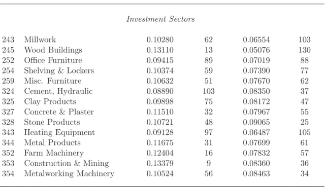
Table 5: Volatility Estimates
SIC Sales Growth Ranking TFP Growth Ranking
Investment Sectors
243 Millwork 0.10280 62 0.06554 103
245 Wood Buildings 0.13110 13 0.05076 130
252 Office Furniture 0.09415 89 0.07019 88
254 Shelving & Lockers 0.10374 59 0.07390 77
259 Misc. Furniture 0.10632 51 0.07670 62
324 Cement, Hydraulic 0.08890 103 0.08350 37
325 Clay Products 0.09898 75 0.08172 47
327 Concrete & Plaster 0.11510 32 0.07967 55
328 Stone Products 0.10721 48 0.09065 25
343 Heating Equipment 0.09128 97 0.06487 105
344 Metal Products 0.11675 31 0.07699 61
352 Farm Machinery 0.12404 16 0.07832 57
353 Construction & Mining 0.13379 9 0.08360 36
Table 5: (continued)
SIC Sales Growth Ranking TFP Growth Ranking
355 Special Industry Machinery 0.11449 34 0.08322 41
356 General Industry Machinery 0.09665 83 0.07220 81
357 Computer Equipment 0.15876 2 0.12395 1
358 Refrigeration Machinery 0.09309 94 0.06565 102
361 Electr. Distrib. Equipment 0.09918 74 0.07199 84
362 Electrical Apparatus 0.09969 70 0.07462 75
366 Communication Equipment 0.11918 26 0.09439 15
374 Railroad Equipment 0.18537 1 0.09023 26
381 Navigation Equipment 0.11408 35 0.09154 22
382 Measuring Instruments 0.09520 86 0.08039 52
Durable Consumption Sectors
227 Carpets & Rugs 0.10379 58 0.06267 113
231 Men’s Suits & Coats 0.11826 27 0.09100 24
251 Household Furniture 0.08932 102 0.05710 126
273 Books 0.07374 123 0.06419 107
274 Misc. Publishing 0.07167 126 0.08340 38
316 Luggage 0.11053 42 0.08945 28
322 Glass & Glasware 0.07177 125 0.05942 121
348 Small Arms & Ammo 0.12910 14 0.10458 8
363 Households Appliances 0.10724 46 0.07423 76 365 Households Audio-Video 0.12339 18 0.09520 13 375 Motorcycles, Bicycles 0.12012 24 0.09396 16 379 Misc. Transportation 0.13299 11 0.06957 90 385 Ophthalmic Goods 0.09895 76 0.09457 14 387 Watches, Clocks 0.11230 37 0.07968 54
391 Jewelry & Silverware 0.10831 44 0.08127 49
393 Musical Instruments 0.08243 113 0.06352 109
394 Dolls, Toys, & Games 0.11467 33 0.08337 40
Nondurable Consumption Sectors
202 Dairy Products 0.07950 117 0.05650 127
203 Canned Fruits & Vegetables 0.10232 66 0.07838 56
204 Grain Mill Products 0.09375 92 0.07213 83
205 Bakery Products 0.06991 127 0.06070 119
206 Sugar 0.09798 77 0.07500 73
207 Fats & Oils 0.12118 21 0.09674 12
208 Beverages 0.09384 91 0.07738 60
Table 5: (continued)
SIC Sales Growth Ranking TFP Growth Ranking
212 Cigars 0.09491 88 0.06254 115 213 Chewing Tobacco 0.07677 118 0.08065 51 225 Knitting Mills 0.12179 19 0.08169 48 232 Men’s Clothing 0.12381 17 0.09891 10 234 Women’s Underwear 0.10716 49 0.09287 19 236 Girls’ Outerwear 0.12010 25 0.10478 7 271 Newspapers: Publishing 0.03780 133 0.05047 131 272 Periodicals: Publishing 0.07673 119 0.07291 79 283 Drugs 0.10269 65 0.09825 11
284 Detergents & Cosmetics 0.09316 93 0.07635 65
291 Petroleum Refining 0.08590 108 0.05521 128
299 Misch. Petroleum 0.09132 96 0.06841 96
301 Tires 0.08837 106 0.06074 118
314 Footwear 0.12151 20 0.07772 59
Other Consumption Sectors (no service life information)
214 Tobacco Stemming 0.15666 3 0.09972 9 221 Cotton Fabric 0.10063 67 0.07074 87 222 Silk Fabric 0.08886 104 0.05795 124 223 Wool Fabric 0.09795 78 0.07520 72 224 Narrow Fabric 0.08507 110 0.06589 101 226 Dyeing Textiles 0.11155 39 0.07652 63
228 Yarn & Thread Mills 0.10274 64 0.06134 117
229 Misc. Textile Goods 0.09926 73 0.07291 78
233 Women’s Outerwear 0.13566 7 0.10947 5
235 Hats & Caps 0.10723 47 0.08120 50
237 Fur Goods 0.06940 128 0.04087 133
238 Misc. Apparel 0.12047 22 0.09271 20
239 Misc. Textiles 0.10541 53 0.07578 67
244 Wood Containers 0.09968 71 0.06894 92
249 Misc. Wood Products 0.10526 55 0.07621 66
261 Pulp Mills 0.07413 122 0.07279 80
262 Paper Mills 0.06812 129 0.05839 123
263 Paperboard Mills 0.06706 130 0.06347 111
265 Paperboard Containers 0.06024 131 0.04087 132
267 Converted Paper Products 0.07314 124 0.05732 125
275 Commercial Printing 0.07514 121 0.06162 116
276 Business Forms 0.06022 132 0.05176 129
277 Greeting Cards 0.08253 112 0.08657 30
Table 5: (continued)
SIC Sales Growth Ranking TFP Growth Ranking
279 Services for Printing 0.08157 114 0.08247 44
281 Inorganic Chemicals 0.11076 40 0.10638 6 282 Plastic Materials 0.09113 98 0.07219 82 286 Organic Chemicals 0.09712 81 0.08541 32 287 Agricult. Chemicals 0.13484 8 0.11162 4 289 Misc. Chemicals 0.10044 68 0.08320 42 302 Rubber Footwear 0.13218 12 0.08337 39 305 Packing Devices 0.08365 111 0.07169 85 306 Rubber Products 0.08877 105 0.06351 110
308 Misc. Plastic Products 0.09511 87 0.06815 97
311 Leather Finishing 0.11066 41 0.07547 70
313 Shoe Cut Stock 0.11712 28 0.05930 122
315 Leather Gloves 0.10528 54 0.08004 53
317 Handbags 0.12864 15 0.08220 45
319 Other Leather Goods 0.10306 61 0.08991 27
321 Flat Glass 0.09015 100 0.07555 68 323 Glass Products 0.09988 69 0.06740 99 341 Metal Cans 0.09936 72 0.06542 104 342 Cutlery 0.08111 116 0.06443 106 346 Metal Forging 0.09790 80 0.06303 112 369 Electrical Equipment 0.10743 45 0.07637 64
395 Pens & Pencils 0.08148 115 0.06620 100
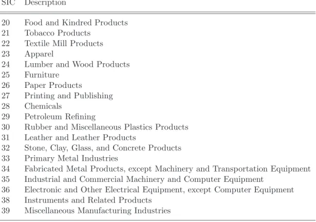
Table 6: 1987 SIC
SIC Description
20 Food and Kindred Products 21 Tobacco Products
22 Textile Mill Products
23 Apparel
24 Lumber and Wood Products 25 Furniture
26 Paper Products
27 Printing and Publishing
28 Chemicals
29 Petroleum Refining
30 Rubber and Miscellaneous Plastics Products 31 Leather and Leather Products
32 Stone, Clay, Glass, and Concrete Products 33 Primary Metal Industries
34 Fabricated Metal Products, except Machinery and Transportation Equipment 35 Industrial and Commercial Machinery and Computer Equipment
36 Electronic and Other Electrical Equipment, except Computer Equipment 38 Instruments and Related Products
39 Miscellaneous Manufacturing Industries
References
Abraham, A., and K. White(2006): “The Dynamics of Plant–Level Productivity in US Manufacturing,” Census Bureau Working Paper #06-20.
Aghion, P., N. Bloom, R. Bludell, R. Griffith, and P. Howitt (2005): “Competition and Innovation: An Inverted-U Relationship,” Quarterly Journal of Economics, 120(2), 701–728.
Aghion, P., C. Harris, P. Howitt, and J. Vickers(2001): “Competition, Im-itation, and Growth with Step–by–Step Innovation,” Review of Economic Studies, 68, 467–492.
Aghion, P., and P. Howitt (1992): “A Model of Growth through Creative De-struction,” Econometrica, 60, 323–51.
Bachman, R., and C. Bayer (2009): “Firm-Specific Productivity Risk over the Business Cycle: Facts and Aggregate Implications,” University of Michigan. Baily, M. N., E. J. Bartelsman, and J. Haltiwanger(2001): “Labor
Produc-tivity: Structural Change And Cyclical Dynamics,” The Review of Economics and Statistics, 83(3), 420–433.
Baily, M. N., C. Hulten, and D. Campbell(1992): “Productivity Dynamics in Manufacturing Plants,” Brooking Papers on Economic Activity: Microeconomics, 4(1), 187–267.
Bartelsman, E. J., and W. Gray (1996): “The NBER Manufacturing Produc-tivity Database,” NBER Technical Working Papers 0205, National Bureau of Eco-nomic Research, Inc.
Bils, M., and Y. Chang (2000): “Understanding how price responds to costs and production,” Carnegie-Rochester Conference Series on Public Policy, 52(1), 33–77. Bils, M., andP. J. Klenow (1998): “Using Consumer Theory to Test Competing
Business Cycle Models,” Journal of Political Economy, 106(2), 233–261.
(2004): “Some Evidence on the Importance of Sticky Prices,” Journal of Political Economy, 112(5), 947–985.
Caggese, A. (2008): “Entrepreneurial Risk, Investment and Innovation,” Universi-tat Pompeu Fabra.
Campbell, J. Y., M. Lettau, B. G. Malkiel, and Y. Xu (2001): “Have Indi-vidual Stocks Become More Volatile? An Empirical Exploration of Idiosyncratic Risk,” Journal of Finance, 56(1), 1–43.
Castro, R., G. L. Clementi, and G. MacDonald (2004): “Investor Protec-tion, Optimal Incentives, and Economic Growth,” Quarterly Journal of Economics, 119(3), 1131–1175.
(2009): “Legal Institutions, Sectoral Heterogeneity, and Economic Develop-ment,” Review of Economic Studies, 76(2), 529–561.
Chang, Y., andJ. Hong(2006): “Do Technological Improvements in the Manufac-turing Sector Raise or Lower Employment?,” American Economic Review, 96(1), 252–368.
Chun, H., J.-W. Kim, R. Mork, and B. Yeung (2008): “Creative Destruction and Firm–Specific Performance Heteroeneity,” Journal of Financial Economics, 89, 109–135.
Clementi, G. L., and T. Cooley (2009): “Executive Compensation: Facts,” NBER Working Paper # 15426.
Clementi, G. L., and H. A. Hopenhayn (2006): “A Theory of Financing Con-straints and Firm Dynamics,” The Quarterly Journal of Economics, 121(1), 229– 265.
Comin, D., and S. Mulani (2006): “Diverging Trends in Aggregate and Firm Volatility,” The Review of Economics and Statistics, 88(2), 374–383.
Comin, D., and T. Philippon(2005): “The Rise in Firm-Level Volatility: Causes and Consequences,” NBER Macroeconomics Annual, 20.
Copeland, A.,andA. Shapiro(2010): “The Impact of Competition on Technology Adoption: An Apples-to-PCs Analsyis,” Federal Reserve Bank of New York. Cu˜nat, A., and M. J. Melitz (2010): “Volatility, Labor Market Flexibility, and
the Pattern of Comparative Advantage,” Journal of the European Economic Asso-ciation, forthcoming.
Cummins, J. G., and G. L. Violante (2002): “Investment-Specific Technical Change in the United States (1947-2000): Measurement and Macroeconomic Con-sequences,” 5(2), 243–284.
Davis, S., J. Haltiwanger, and S. Schuh(1996): Job Creation and Job Destruc-tion. MIT Press, Cambridge, MA.
Davis, S. J., J. Haltiwanger, R. Jarmin, and J. Miranda (2006): “Volatility and Dispersion in Business Growth Rates: Publicly Traded versus Privately Held Firms,” NBER Macroeconomics Annual, 21, 107–156.
Dunne, T., J. Haltiwanger, and K. R. Troske (1997): “Technology and jobs: secular changes and cyclical dynamics,” Carnegie-Rochester Conference Series on Public Policy, 46(1), 107–178.
Ericson, R., andA. Pakes(1995): “Markov–Perfect Industry Dynamics: A Frame-work for Empirical Work,” Review of Economic Studies, 62, 53–82.
Evans, D.(1987): “The Relationship between Firm Growth, Size and Age: Estimates for 100 Manufacturing Firms,” Journal of Industrial Economics, 35, 567–81. Foster, L., J. Haltiwanger, and C. Krizan (2001): “Aggregate Productivity
Growth: Lessons from Microeconomic Evidence,” in New Developments in Produc-tivity Analysis, ed. by C. R. Hulten, E. R. Dean, and M. J. Harper, pp. 303–363. University of Chicago Press.
Gourio, F. (2008): “Estimating Firm–Level Risk,” Boston University.
Hall, B. (1987): “The Relationship between Firm Size and Firm Growth in the US Manufacturing Sector,” Journal of Industrial Economics, 35, 583–606.
Herranz, N., S. Krasa, andA. P. Villamil(2009): “Small Firms in the SSBF,” Annals of Finance, 5, 341–359.
Hopenhayn, H. A. (1992): “Entry, Exit and Firm Dynamics in Long Run Equilib-rium,” Econometrica, 60, 1127–50.
Michelacci, C., andF. Schivardi(2008): “Does Idiosyncratic Business Risk Mat-ter?,” CEPR Discussion Papers 6910, C.E.P.R. Discussion Paper.
Quadrini, V. (1999): “Entrepreneurship, Saving, and Social Mobility,” Review of Economic Dynamics, 3(1), 1–40.
(2003): “Investment and Liquidation in Renegotian–Proof Contracts with Moral Hazard,” Journal of Monetary Economics, 51, 713–751.
Samaniego, R. (2009): “Entry, Exit and Investment–Specific Technical Change,” American Economic Review, 100(1), 164–192.
Syverson, C. (2004): “Market Structure and Productivity: A Concrete Example,” Journal of Political Economy, 112(6), 1181–1222.