Duclos: Institut d’Anàlisi Econòmica (CSIC), Barcelona, Spain, and Département d’économique and CIRPÉE, Université Laval, Canada
Leblanc: Department of Finance, Ottawa, Canada [email protected]
Sahn: Cornell University, Cornell, USA
Cahier de recherche/Working Paper 09-10
Comparing Population Distributions from bin-Aggregated Sample
Data: an Application to Historical Height Data from France
Jean-Yves Duclos Josée Leblanc David Sahn
Abstract:
This paper develops a methodology to estimate the entire population distributions from bin-aggregated sample data. We do this through the estimation of the parameters of mixtures of distributions that allow for maximal parametric flexibility. The statistical approach we develop enables comparisons of the full distributions of height data from potential army conscripts across France’s 88 departments for most of the nineteenth century. These comparisons are made by testing for differences-of-means stochastic dominance. Corrections for possible measurement errors are also devised by taking advantage of the richness of the data sets. Our methodology is of interest to researchers working on historical as well as contemporary bin-aggregated or histogram-type data, something that is still widely done since much of the information that is publicly available is in that form, often due to restrictions due to political sensitivity and/or confidentiality concerns.
Keywords: Health, health inequality, aggregate data, 19th century France, welfare
1 Introduction
There are many reasons to consider dimensions of well-being other than in-come or expenditure, both normative and practical. Following Sen (1985) and others, for example, one may wish to consider well-being as multidimensional, comprising characteristics such as , good health, nutrition, literacy, and freedom of association. Income may be instrumentally important to achieve these ends, but it is the capabilities themselves that are intrinsically important and merit recogni-tion and measurement in their own right. Poverty can thus be defined as depriva-tion of basic capabilities or the failure of certain basic funcdepriva-tionings, not just low levels of income. Deprivation of capabilities can also in turn contribute to low material standards of living.
This paper focuses on health, which is certainly important in a multidimen-sional understanding of well-being. In fact, even in a purely unidimenmultidimen-sional wel-farist framework, it can be argued that health contributes to welfare at least as much as income. Income may not even be a sound directional indicator of overall welfare in some environments. As Floud (1984) writes, “[t]here is little point in an improvement in real wages which is bought at the expense of a miserable life and an early death”. The example of the United States, for instance, shows that although health and economic growth have generally converged during the twenti-eth century, they diverged during the nineteenth century (“the antebellum period”) (Costa and Steckel 1997); strong economic growth during the nineteenth century coincided inter alia with a decrease in body-heights. Whether income is more indicative of welfare than health in such circumstances is then open to debate.1
Beyond the conceptual arguments, there are many practical reasons to mea-sure well-being in non-income dimensions. First, meamea-surement difficulties may be less of a problem for some non-income variables. Collecting income (or expen-diture) data is a complex procedure that contrasts, for instance, with the relatively straightforward procedure of collecting anthropometric data — data that also suf-fer typically less from misreporting. Measurement errors can of course still affect such data, but anthropometric data (unlike other self-reported and subjective mea-sures of health) are more likely to be uncorrelated with important variables of interest — such as the welfare variable itself. Note also that health can be more 1More generally, measures of health are often not highly correlated with incomes, either within
a given country or across countries (Haddad and Ahmed 2003, Behrman and Deolalikar 1988, Behrman and Deolalikar 1990, Appleton and Song 1999), suggesting among other things that health variables may provide significant information on welfare that is not captured by income alone.
easily measured at the individual rather than at the household level, thus largely avoiding the need to make difficult assumptions on the well-being of individuals which requires an assessment of both the needs of individuals and how resources are allocated among household members relative to needs.
Perhaps most importantly, the choice of a welfare indicator obviously depends on the availability of data. Research on the distribution of well-being routinely takes advantage of the availability of large-scale micro-data sets that provide de-tailed information on money-metric and non-monetary indicators2. The choice of welfare indicators is much more constrained for studies covering earlier historical periodswhere the available data is more limited and often of variable quality. It may for instance be the case that only part of the initially gathered welfare infor-mation was preserved, or that it comes from sources whose primary goal was not to capture data representative of the population3. Furthermore, historical house-hold level data on incomes and expenditures are particularly difficult to collect since economies were less monetized, transactions were often in-kind, consump-tion was largely from home consumpconsump-tion rather than market purchases, and tax authorities did not have good records of gathering and verifying information on incomes.
Fortunately, quality historical data are widely available from many countries on one of the clearest manifestations of health and nutritional status, stature. It is also now well established that one of the best global indicators of living condi-tions is height, standardized for age and gender (de Onis, Frongillo, and Blossner 2000). More specifically,stature is the outcome of a combination of inputs that affect nutrition and disease, such as the local health environment, access to clean 2Some of the non-monetary indicators found in the literature include body-height (Fogel,
En-german, Floud, Steckel, Trussell, Wachter, Sokoloff, Villaflor, Margo, and Friedman 1982, Steckel and Floud 1997, Wagstaff 2002, Pradhan, Sahn, and Younger 2003, Sahn and Younger 2005), body mass index (Costa and Steckel 1997), amount of abdominal fat (Costa and Steckel 1997), birth weight (Costa 1999), life expectancy (Whitwell, Souza, and Nicholas 1997, Goesling and Firebaugh 2004), the overall mortality rate or mortality before a certain age (Costa and Steckel 1997, Floud and Harris 1997, Weir 1997, Whitwell, Souza, and Nicholas 1997, Wagstaff 2002), the prevalence of chronic or severe illness (Costa and Steckel 1997, Wagstaff 2002, Anson and Sun 2004), the individual’s own assessment of his or her health (Deaton and Paxson 1998, Nolte and McKee 2004), disabilities (Anson and Sun 2004), difficulties accomplishing tasks (Anson and Sun 2004), and mental illness (Anson and Sun 2004).
3For example, Costa (1999)’s data on the birth weight of babies were obtained from hospital
archives. These archives are not necessarily complete, since hospitals will not have kept every patient file since 1848; moreover, the hospital registries may represent a biased sample of the pop-ulation, since wealthier women were over-represented among those who gave birth in hospitals.
water, nutrient intake, maternal health status, health technology, the organization of work, and so forth. In short, stature captures “multiple dimensions of the indi-vidual health and development and their socio-economic and environmental deter-minants” (Beaton, Kelly, Kevany, Martorell, and Mason 1990)4. And in particular, heights of young men entering adulthood is a cumulative indicator of their overall health and nutritional status during their formative years, particularly the period prior to the beginning of puberty.
Economic historians have thus expended considerable effort to examine changes in anthropometric outcomes of various populations over time (Fogel, En-german, Floud, Steckel, Trussell, Wachter, Sokoloff, Villaflor, Margo, and Fried-man 1982, Steckel and Floud 1997, Weir 1997, Deaton and Paxson 1998 and Goesling and Firebaugh 2004).5 An important concern that arises in how histo-rians use anthropometric indicators is whether the summary health statistics they employ, particularly measures of central tendencies, can adequately capture the
distribution of health. Indeed, it is increasingly recognized that looking at
en-tire distributions of health, just as economists have long done with incomes, can provide valuable information that would otherwise be hidden by summary health statistics, such as means and the share of the population that falls before a norma-tive standard, or cut-off point, that may define poor health6.
This paper gives prominence to the distributional analysis of health by exam-ining both the evolution and the distribution of heights throughout France in the nineteenth century. More specifically, the paper uses a particularly rich data set collected on men who were called up for possible conscription into the French army during this period. The screening of all men at the age of 20 for manda-4This is also supported by the existence of a significant correlation between body-heights and
various indicators of health — see for instance Wagstaff (2002) — suggesting that the choice of an indicator other than body-height would yield similar results. Moreover, adult stature is not only a good indicator of prior episodes of, infection and chronic disease, but it has also been shown to be an important determinant of risk of morbidity and mortality.
5A number of other studies have also looked at health inequalities, using statistics such as
covariances (such as Deaton and Paxson 1998 and Anson and Sun 2004), differences between various percentiles (Costa 1999), distances from the mean for different social classes (Anson and Sun 2004), or inequality indices (e.g., Wagstaff 2002, Pradhan, Sahn, and Younger 2003, Goesling and Firebaugh 2004, Sahn and Younger 2005). Studies of health inequality have also attempted to explain whether inequality in some factors, such as income, can transmit itself into health inequal-ity — see for instance Weir (1997), Anson and Sun (2004), and Nolte and McKee (2004)). Other studies have decomposed the evolution of health inequality across factors, such as Pradhan, Sahn, and Younger (2003), Goesling and Firebaugh (2004), Sahn and Younger (2005), and Wagstaff (2002).
tory military service involved a physical examination, including measuring their height. Thus, we have a virtually complete census of heights for each year, dis-aggregated by administrative department. Data in such abundance for a whole century are arare find. Consequently, socio-economic improvements as well as periods of adverse conditions in 19th-century France can be expected to have an observable effect measured by the stature achieved at 20 years of age - which is what we measure in our data.
While individual heights were recorded at the time of conscription, the data we have available are limited to the number of men that fall into classes, or bins of height intervals, for each year and department. This raises obvious challenges given our objective to compare the entire distributions of heights. These difficul-ties are not unique to our data, or the paper’s historical period of interest. Even today, much of the information that is used and publicly available on distributions of income come from bin-aggregated, or histogram-type, data — important exam-ples of this are the popular World Income Inequality and POVCAL databases7. In several countries, the unit data from early household surveys have not survived; in other cases, access to distant and/or more recent microdata is restricted by politi-cal sensitivity and confidentiality concerns. We therefore propose and implement a method that estimates the entire population distributions from the bin-aggregated sample data through the estimation of the parameters of mixtures of distributions that allow for maximal parametric flexibility8. While we only apply our method to the historical height data from France, this approach will be of general interest to both historians and other researchers working on contemporary bin level data on household incomes, heights, and other indicators of well-being.
Our data are abundant, consisting of more than 6000 different distributions of heights for the period 1819 to 1900 over 90-some departments. Using the sampling distribution of the estimators of the means and of the cumulative dis-tributions of heights, we test for differences in means and also implement tests for robust comparisons across time and regions. We are also able to correct our inference procedures for the possible presence of measurement errors. This is rarely possible to do with the usual data used for comparing welfare; it is made feasible here by the richness of the data. We correct for measurement errors by measuring and taking into account the noise that is (possibly) introduced by mea-surement errors in the many year-to-year comparisons of the distributions that are
7Seewww.wider.unu.edu/wii d/wiid.htmandwww.worldbank.or g/LSMS/tools/povcal/ 8See for instance Bandourian, McDonald, and Turvey (2002) for a review of some of the more
made possible by our data. This renders the broader comparisons in which we are interested robust to both sampling and measurement errors. Again, this is done by estimating the parameters of mixtures of distributions with the maximum degree of parametric flexibility and by therefore exploiting all the statistical information that is present in the available height data.
In short, this paper develops a methodology that allows us to estimate the en-tire population distributions from the bin-aggregated sample data. We go on to illustrate how this methodology can be applied to a rich data set from France of 20-year-old army conscripts, and thereafter employ the generated distributions to address one of many possible questions on the evolution and the distribution of health and welfare in 19th-century France. These data are introduced in Section 2. The methodology for deriving from bin data the entire distribution as well as the average height of each department-year is described in Section 3.1 and extracts the maximum possible amount of information from the data. Statistical tests of differences in mean heights and in the entire distributions are performed using the test statistics and sampling distributions presented in Section 3.2. Further details in carrying out stochastic dominance tests appear in Section 3.3. The empirical results are presented in Section 4, where two main questions are more particu-larly considered to illustrate how our statistical procedures can be used. The first question considers the evolution of body-heights in France from the beginning to the end of the century; the second deals with the regional correlates of the distri-bution of body-heights. Section 5 concludes the paper. The Appendix in Section 6 provides more technical details on the data, the estimation procedures, and the adjustment for measurement errors.
2 Data
The data we use are from the registries of potential conscripts into the French army for the period 1819 to 1900, covering the 90-some departments of France9. More precisely, they are from the "Comptes rendus statistiques et sommaires." Depending on the year, they constitute either a "nearly" random sample, or a com-plete census of young French men aged 20 years old for each year of the century (this point is addressed in greater detail in the Appendix on page 22). They consist of 6369 different datasets, each representing the distribution of body-heights for a 9We are very grateful to Gilles Postel-Vinay for his generous assistance in making available to
us, and helping us better understand the data. More details on the data set are also found in Sahn and Postel-Vinay (forthcoming).
given department and a given year. In total, we have measurements on close to 15 million young French men over the course of the century.
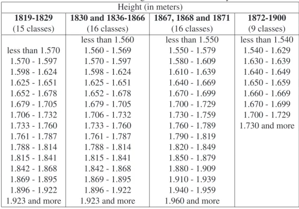
A particularity of these data is that they are not available in a totally disag-gregated form. Rather, they are grouped into "classes," each of which contains individuals within a specific body-height range. The available data thus report the number of individuals in each of these classes. Furthermore, neither the number of classes, nor the boundaries between bins, were constant throughout the century. The data from 1819 to 1829 are divided into 15 classes, those from 1830 to 1871 into 16 classes, and those from 1872 to 1900 into 9 classes. The class boundaries for the various years are reproduced in Table 1. Note that the classes were based on the old imperial measurements until 1867 (1 French inch = 27.07 millimeters) so that 1.570 meters corresponds to 4 feet 10 inches, 1.597 meters to 4 feet 11 inches, etc. The metric measurements we employ are the public equivalent to the imperial measurements used during these years.
These registries contain a considerable amount of information. Indeed, the number of conscripts measured each year varies between one-quarter, and all, of the male population aged 20. Between 1819 and 1830, approximately 80,000 men were measured each year; from 1836 to 1885, approximately 150,000; and as of 1886, approximately 300,000. Only during this final period was the entire male population aged 20 measured each year.
3 Estimation and inference
3.1 Estimation of complete distributions
That the data available for this study are grouped into classes raises difficulties if the objective is to compare complete distributions of heights. To address this challenge, we first need to estimate the continuous population height distributions using the discontinuous sample histograms that are available. To do this, we solve a system of (C − 1) equations in (C − 1) unknowns, where C is the number of classes into which the heights are regrouped in the aggregated sample data. Each of these equations captures the probability of belonging to one of the C classes of height. Equation (1) defines such a probability for the class c of heights x, a class whose lower bound is xcand upper bound is xc:
where F stands for the height distribution function, ˆΘ is the vector of the estimated parameters for this function, and ˆHcis the proportion of heights between xcand
xcthat is observed in our data.
F is specified as a mixture of normal distributions, namely, as a weighted
sum of several normal distributions. We let the mixture use as many parameters as is statistically possible given the grouped form of our data. This mixture of normal distributions thus allows for the maximal possible amount of estimation flexibility. Note that since the normal distribution is smooth, this property will also be imposed on our estimated population height distributions.
Equation (2) provides an example of a “mixture” of three normal distributions with a set of 9 parameters:
F (x; α1, α2, α3, µ1, µ2, µ3, σ1, σ2, σ3) = α1 Φ µ x − µ1 σ1 ¶ + α2 Φ µ x − µ2 σ2 ¶ + (1 − α1− α2) Φ µ x − µ3 σ3 ¶ , (2) where Φ is the distribution function of the standard normal distribution, and where
αd, µd and σd correspond respectively to the weight, the mean, and the standard
error of normal distribution d. Note that since α1 + α2 + α3 = 1, we can set
α3 = 1 − α1 − α2. There are therefore 8 “free” parameters in (2). Thus, a mixture of D ≥ 1 normal distributions contains 3D−1 free parameters. Similarly, there are only (C − 1) “degrees of freedom” in data aggregated into C classes of heights, since the probabilities of belonging to one class is one minus the sum of the probabilities of belonging to the others. Hence, the problem is to solve a system of equations such as (1), with c = 1, . . . , C − 1, using the ˆHc observed
probabilities of belonging to C classes and choosing D = C/3.
For some years, however, C/3 is not an integer. For those years we use instead mixtures of (C + 1)/3 or (C + 2)/3 distributions, setting the last one (σC+1)
or two (µC+2 and σC+2) parameters in the mixture to some pre-specified values.
These values are chosen as those that are estimated in the 1880 distribution of individual heights, which is the only year for which we have access to the entire set of individual-level data.
More technical details on the above estimation procedure can be found in the Appendix, Section 6.2.
3.2 Test statistics
Once the parameters ˆΘ in (1) are estimated for each year and each department, we can proceed to assess the evolution of the distributions of health in nineteenth-century France. We do this in two ways: first by comparing mean body-heights, which is one of the most common procedures in the literature, and second by comparing “health poverty rates”. Note that these poverty rates will be compared across ranges of possible “health poverty lines”, which will amount to testing for stochastic dominance of height distributions.
Mean height can be estimated as ˆ
µ =
Z ∞
−∞
x dF (x; ˆΘ). (3)
The height poverty rate (“the poverty headcount”) is the proportion of individuals below a height poverty line. Computing the poverty rate consists of evaluating the distribution function at the poverty line z:
F (z; ˆΘ) = Z z
−∞
dF (x; ˆΘ). (4)
Once estimated, ˆµ and F (z; ˆΘ) can be compared across departments and years. For the comparisons of means, the null hypothesis is that the mean of distribution
B does not exceed the mean of distribution A, and the alternative hypothesis is
that it does. The test statistic that we use is then ˆ µB− ˆµA p d var(ˆµB) + dvar(ˆµA) (5) where d var(ˆµ) = 1 n Z ∞ −∞ (x − ˆµ)2 dF (x; ˆΘ) (6)
and n (which is always well above 500 in our data) stands for the number of sol-diers over whom the aggregated bin data have been computed. Under the assump-tion that populaassump-tion heights follow the flexible form given by (2) and that the two means µBand µAare equal, the statistic (5) can be shown to follow asymptotically
a normal distribution with mean zero and unit variance. At the conventional 5% level, the above null hypothesis will then be rejected if (5) is greater than 1.645.
For ordering poverty headcounts10, we use the test statistic F (z; ˆΘA) − F (z; ˆΘB) q d var(F (z; ˆΘB)) + dvar(F (z; ˆΘA)) (7) where d var(F (z; ˆΘi)) = F (z; ˆΘi) (1 − F (z; ˆΘi)) n . (8)
Under the null hypothesis of equality of the two distribution functions at z, and that population heights follow the flexible form given by (2), the distribution of F (z; ˆΘA) − F (z; ˆΘB) is asymptotically normal with mean 0 and variance
d
var(F (z; ˆΘB)) + dvar(F (z; ˆΘA)) (since the samples from A and B are
indepen-dent).
Note that the expressions ˆµ, dvar(ˆµ), F (z; ˆΘA) and dvar(F (z; ˆΘi)) are readily
computed once the parameters ˆΘ in system (1) are estimated. Since ˆΘ contain the maximal number of parameters that can be estimated from our data, these statistics are also as distribution-free as they can be. Note furthermore that the asymptotic result for (7) is valid for the z located at the frontiers of the bins of the aggregated data even when population heights do not follow exactly the flexible form given by (2), since at such z we can estimate (7) and (8) directly from the ˆHcin (1).
3.3 Dominance tests
A poverty comparison that uses (7) depends on the choice of the line z. It is also evidently dependent on the choice of the distribution function as a “poverty index”. To make the paper’s poverty comparisons more robust to such choices, stochastic dominance tests can be performed by comparing poverty rates over ranges of poverty lines. Pushing this approach farther, one can also compare cu-mulative height distributions over the entire range of possible heights.
To see what this implies in terms of poverty rankings, note that the poverty headcount F belongs to a general class of poverty indices, denoted as Π1(z+), that can be defined with the help of two simple axioms and of a condition (see for instance Duclos and Araar 2006, Part III). The first axiom, a monotonicity axiom, says that an increase in the body-height of any one individual (provided that no one else’s body-height decreases) should (weakly) reduce the value of a poverty
index. The second axiom, a symmetry axiom, says that interchanging the body-height of any two individuals should not affect the poverty index. The condition is that the poverty index should use a poverty line that is below z+.
We then say that distribution B poverty dominates11distribution A if and only if the distribution function for B lies below that for A for all poverty lines in the interval [0, z+]. Analytically, for generally-denoted poverty indices P (z) and a distribution function F (x), we have
PA(z) ≥ PB(z) ∀ P (z) ∈ Π1(z+)
⇔ FA(x) ≥ FB(x) ∀ x ∈ [0, z+]. (9)
This results says that ordering poverty headcounts over all lines in [0, z+] also ranks all poverty indices that meet the monotonicity and symmetry axioms, and for whatever choice of poverty lines below z+.
For statistical and normative reasons (see Davidson and Duclos 2006), these dominance tests are better implemented over ranges poverty lines ranging from of
z−to z+, rather than from 0 to z+(these tests are then denoted in the literature as restricted stochastic dominance tests). Empirically, this interval will correspond to [1.53, 1.78], or from approximately the 3rd to the 97th percentile of the distri-butions of heights observed in nineteenth century France. The null and alternative hypotheses for the dominance tests that we conduct can then be written as:
H0 : F (z1; ˆΘA) ≤ F (z1; ˆΘB) or F (z2; ˆΘA) ≤ F (z2; ˆΘB) or . . . or F (zm; ˆΘA) ≤ F (zm; ˆΘB) (10) versus H1 : F (z1; ˆΘA) > F (z1; ˆΘB) and F (z2; ˆΘA) > F (z2; ˆΘB) and . . . and F (zm; ˆΘA) > F (zm; ˆΘB), (11)
11In the first order, since we could also test for higher-order dominance comparisons — see
where the zi’s represent m points in the interval [z−, z+]. The null hypothesis is
an hypothesis of non-dominance of A by B. The alternative hypothesis is that B dominates A.
The decision rule differs from that for simpler test hypotheses, since H0 and
H1are sets of multiple hypotheses. The decision rule is to reject H0and conclude that B dominates A if and only if each of the inequalities in H0can be rejected at the 5% level. Since it involves testing separately over m hypothesis tests, this test procedure is generally conservative: the 5% nominal level for each inequality test in H0 leads to a less than 5% probability of committing a Type I error of wrongly rejecting the joint hypothesis of non-dominance of A by B when non-dominance is true.
An illustration of a test procedure for stochastic dominance is provided by Figure 1, which uses data from the Ain department. We test here whether distri-bution B (1886) dominates distridistri-bution A (1819) (H0: 1886 does not dominate 1819). We see in the lower panel that the t test statistics (of equation (7)) exceed the critical value (the dotted line) across the entire interval [1.53, 1.78], so we can reject H0and conclude that year 1886 dominates year 1819, that is, that year 1886 has less height for whatever choice of poverty measures in Π1(z+).
4 Results
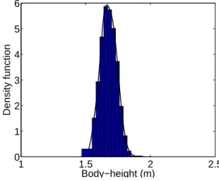
We now turn to the empirical results. Recall that the first step is to estimate an entire population distribution function for each of our 6369 datasets. This is done using the estimation techniques presented in Section 3. Once estimated, these distributions generally fit the empirical distributions very well, as is illustrated for instance in Figure 2. The histogram shows rectangles whose area ˆHc (see
(1)) comes from the aggregated data. The line is the estimated density function, a mixture of normal density functions (whose cumulative distributive functions appear in (2)).
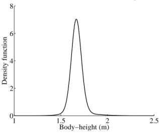
Some estimated distributions are very close to the normal distribution, such as the one of Figure 3. This is more often the case of the distributions with eight parameters (a mixture of three normal distributions), e.g., for many of the dis-tributions from 1872 to 1900. Other disdis-tributions are less smooth, as Figure 4 shows. It proved impossible to find a satisfactory solution to the system (1) for 3 out of the 6369 distributions of our database. This may be due to numerical limi-tations in attempting to solve for systems of up to 15 equations in 15 unknowns, in which each equation is a sum of as many as 6 normal distribution functions —
also computed numerically. It can also be because of difficulties inherent in fitting empirical distributions that diverge (because, e.g., of sampling variability) widely from the normal distribution. Representing less than 0.05% of our distributions, these three distributions are dropped from our analysis; further details on them can be found in Leblanc (2007).
4.1 National distributions of heights
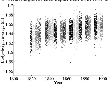
We first consider the overall distribution of heights of the French during the 19th century. Figure 5 illustrates mean body-heights in each department for every year. Observe that there appears to be an upward trend in average body-heights. This phenomenon is most clearly seen in Figure 6, which reproduces the national mean of body-heights (i.e., all departments aggregated — more information can be found in the Appendix) from 1819 to 1900. Note that the national mean seems to have increased from around 163.5 to 165.5 centimeters between 1819 and 1900. Figure 6 also suggests that this evolution of the mean was not constant. Finally, observe in Figure 5 that there is considerable variation across departments.
4.2 Year-to-year comparisons
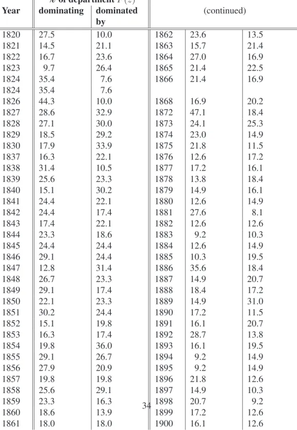
Let us now turn to the year-to-year evolution of heights for each department. For each year, Tables 2 and 3 show the percentage of departments within which this year is better than (or dominates) the preceding year. Table 2 uses means and Table 3 compares distribution functions at a fixed z.
Notice that there appears to be a great deal of variation in the means from year to year. In Table 2, the percentages of departmental means dominating or dominated by the preceding year hover around 15% to 35%. These percentages therefore far exceed 5%, the level of the test (i.e. the proportion of times when sampling error would have erroneously led us to conclude that there was domi-nance when there was in fact none). The percentages of decline are also nearly as high as those of increase.
Similar results in Table 3 are obtained for comparisons of the proportion of individuals whose body-height was below 1.652 meters for the years 1819–1866 and 1.640 meters for 1867–1900.12 The presumption that the variability in the 12These values were selected because they correspond to class boundaries (the proportion used
thus corresponds to the sum of the number of individuals in each class below this boundary) and they differ because the class boundaries were changed between these two periods. They also
means actually springs from the raw data, and not from peculiarities in the esti-mation methods, is thus supported by the fact that a similar dominance rate exists in Table 3 as for means in Table 4.
There are two possible explanations to the relatively high rate of “acceptance” of dominance. The first is that the distributions within a single department truly do vary from one year to the next, and that the null hypothesis of non-dominance of the distributions must naturally be rejected more often than the nominal 5% level of the tests if we want our tests to have some power. The second, more cau-tious, explanation starts with the presumption that there should be little difference from one year to the next between the population distributions within a single de-partment, and that we need to locate the source of the high rates of acceptance of dominance in measurement errors. This would then admonish caution in our interpretations of the dominance results.
The Appendix (Section 6.4) analyzes the effect of various possible sources of measurement errors on the validity of our inference results. A relatively conserva-tive approach that emerges from that analysis is to consider the year-year accep-tance of dominance rankings to stem from department-year-specific measurement errors that are identically, independently and normally distributed across the cen-tury. This would suggest a standard deviation of those measurement errors of the order of 1.7 times the size of the sampling error on the estimator of the mean — or roughly 0.23 cm. Note that a standard deviation of 0.23 cm in the distribution of (true) population average heights would also suffice to generate the high rates of dominance acceptance that we observe in Table 2.
Thus, rather than conclude that one year dominates another on the usual ba-sis of rejecting non-dominance at the nominal level of 5%, we will only draw this conclusion if we can reject non-dominance of means at a nominal level of 20%, which is approximately the average rate of dominance rankings across de-partments from one year to the next over the century. In the case of stochastic (or distribution) dominance (Table 4), the corresponding average rate of dominance rankings is about 1.5%. Even though this is smaller than the 5% nominal level used in testing each of the null in the composite null H0 in (10), recall from the discussion on page 11 that the decision rule is to reject that composite null and conclude that B dominates A only if all of the inequalities in H0 can be rejected at the nominal level. The test procedure is therefore inherently conservative,
lead-correspond to points outside of the tails of these distributions. In fact, approximately 60% of individuals’ body-heights were less than 1.652 meters in 1819, and for 25% body-height was less than 1.640 meters in 1886. Because of this, it is worth noting that only the information present in the data (and not in the estimated distributions) were used for these tests.
ing to a probability of committing a Type I error that can be much lower than the nominal level. Allowing for the presence of measurement errors in our context is not enough to offset this. This explains why the 1.5% quoted above is below the nominal 5% level.
4.3 Did the body-height of the French increase during the 19th
century?
We then turn to the following question: “Did the body-height of the French increase during the 19th century?” To answer this, we compare the distributions of the first ten years of available data (1819–1828) with those of the last ten years (1891–1900) on the basis of the elements discussed above — the means and the entire distributions. Comparisons of department-years were performed ment by department, in order to account for “fixed effects” unique to each depart-ment (slight variations in genetic heritage, different geophysical conditions, etc.). If data are available for all years, this corresponds to a maximum of 100 com-parisons per department. Overall, 7430 individual comcom-parisons were performed. In addition, aggregate analyses were also performed: for these same years, the means and distribution for all of France were compared.
4.3.1 Comparisons of means
Overall, 93.8% of the distributions at the end of the century had a statistically greater mean than at the beginning. Thus, there was clearly a height progression over the course of the century, even in light of the aforementioned conservative-ness of our inference procedures.
One of the reasons why this proportion is not 100% can be found in devel-opments that are specific to certain departments, as Figure 7 illustrates for the Calvados department. We observe that, in this department, the evolution between the beginning and the end of the century is not very pronounced, and that further-more the mean was already high at the start of the century. Figure 8 provides, however, a good illustration for the Ain department of the situation of a vast ma-jority of the departments, namely a steady progression in body-height throughout the century. In addition, for purposes of verification, we identified the percentage of distributions at the beginning of the century that dominated the distributions at the end of the century. This proportion was only 2%, which adds to the strong statistical evidence of an increase in mean height over the course of the century.
Finally, the same test is performed for France as a whole, i.e. we tested for domi-nance of the aggregate means for the years in question. These comparisons reveal a 100% dominance rate of the end of the century over the beginning of the century (and 0% for the beginning over the end). This, again, confirms the strong evidence of a statistically significant increase in mean height.
4.3.2 Dominance tests
In order to test for a stronger normative ranking of the distributions, we test for dominance of end-of-century distributions over start-of-century distributions for values of z ranging from z− = 1.53 to z+ = 1.78 at intervals of 0.0025 (or 101 comparisons per pair of distributions). Using this approach, we find that 35.6% of distributions at the end of the century statistically and stochastically dominated those at the beginning of the century. Even in light of the conservativeness of the inference procedures outlined above, it therefore appears that a robust progression in the distribution of body-heights can be observed during the century. This evo-lution is confirmed by the percentage of dominance “in the other direction” — the dominance of distributions from the beginning of the century over those at the end of the century is near zero (more precisely, 0.02%). This is also confirmed by the evolution of aggregate distributions for each year. Indeed, 100% of distributions for France as a whole at the end of the century dominate those at the beginning of the century (and 0% of those at the beginning dominate those at the end).
Conversely, we see that in the case of poverty rates, the percentage of domi-nance of the end over the start of the century, by department, is substantially less than in the case of the means. This finding that we are less likely to be able to reject the null of non-dominance than the null of equality of means is expected and frequently reported in the literature for anthropometric data (see, for exam-ple, Sahn forthcoming and Sahn and Stifel 2002). The interpretation is that not all percentiles of the distribution benefited equally from improvements in living conditions. However, given that in the rejecting the null of no stochastic domi-nance rests on a very strong criterion, i.e. that no point of distribution A can lie beneath the corresponding point of B if this latter dominates the former, we limit the “rigidity” in comparisons employing bounds z−and z+corresponding to 1.53
and 1.78.
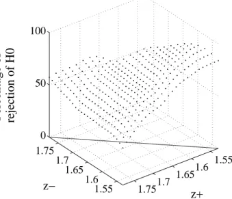
The results are illustrated in Figure 9 (and partially in Table 5). We observe that, in general, the smaller the interval, the greater the proportion of dominance (which makes sense because it reduces the number of inequalities in (11) that must hold). For example, if we restrict the interval to [1.55, 1.75] (approximately
cor-responding to percentiles 8.5 to 95) we obtain 53.1% dominance, or 17.5% more than in the case initially examined. At the limit, if we evaluate this dominance at a single point (the standard definition of a height poverty rate), we obtain a very high percentage of dominance (in the Figure, this corresponds to all points between the ordinate and the 45-degree line in the plane z−z+). For example, if we set the poverty line at 1.57 m, then 98.2% of the time the poverty rate is sta-tistically lower at the end of the century than at the beginning. We also see that if we set the threshold at 1.62 m (as in ?), we obtain end-of-century dominance in 70.4% of cases.
In another vein, it is of some interest to examine Table 6, which shows the differences in the results for stochastic dominance in distribution according to the effective number of points compared in (11). In theory, we should set m to infinity, but in practice this is of course impossible. Instead, we use m = 101. Notice that the difference in the results obtained from between 6 and 101 points is small. Also observe that there is little advantage to using more than 101 points. It is therefore more the range, rather than the fineness of the intervals of thresholds, that matters for testing for height dominance.
Table 5 summarizes the results of the comparison between the beginning and the end of the century. Most decidedly, there is an increase in stature over the course of the century, whether this is assessed using means or distributional dom-inance. However, end-of-century dominance seems much greater when mean body-height is used than when more robust stochastic dominance techniques are applied.
4.4 Are there regional differences in heights?
Let us now turn our attention to showing how our techniques can be employed to address the spatial characteristic of the stature of conscripts. To illustrate, we first examine the question of whether the heights of conscripts from Paris differ from neighboring departments. Next we assess the extent of northeastern and southwestern differences in stature. In both instances, we are interested in the extent to which these differences are observed across the years.
4.4.1 Paris and neighboring departments
In order to assess the height correlate of living in Paris, we conduct a year-by-year comparison of department 7513(which includes Paris) with the neighboring departments 60, 02, 51, 10, 89, 45, 28 and 27.14 These latter are the departments that immediately border the region Île-de-France (the geographical region includ-ing Paris), and they can be located on Figure 10 (where they are underlined). 15
Aggregating across the years, the department of Paris is globally dominated by the bordering departments (Table 7). Indeed, 69.7% of the means of the neigh-boring departments exceed the Paris means (and only 17.0% of the latter dominate the former). Furthermore, 16.4% of the distributions of the adjacent departments stochastically dominate those of Paris (versus 2.5% for the converse). This pro-portion rises to 27.9% (versus 4.8%) if the dominance tests are restricted to the interval [1.55, 1.75]. This supports the results obtained previously by other re-searchers regarding the poorer quality of life in Paris in the nineteenth century.
Figure 11 contrasts the evolution of the means in the department of Paris with those of neighboring departments across the century. There appear to be three distinct periods: one that lasted until 1830, another that ended in approximately 1886 (or 1890), and a final one until 1900. Between 1819-30, 56.6% (versus 21.7%) of means and 8.4% (versus 3.6%) of distributions for Paris dominate those of the other departments. This last percentage increases to 16.9 (versus 6.0) if we compare dominance curves on the interval [1.55, 1.75]. This could be attributable to the fact that, at the beginning of the century, the positive economic effects of the population concentration dominated the negative effects of crowding, such as increased infectious disease, as Paris had yet to become nearly as highly densely populated as it would become later in the century.
Statistical tests for the years 1836-1886, like those for the entire century, in-dicate that the bordering regions dominate Paris at an even more convincing rate: 82.1% (versus 5.6%) of the means of the other departments dominate those of Paris and 20.7% (versus 0.0%) of the neighboring departments dominate Paris in distribution. In the last part of the century (1890-1900), however, we obtain more qualified results. Indeed, 58.0% (versus 28.4%) of the bordering depart-ments dominate Paris in means. But as we have stressed throughout this paper,
13Seine.
14Oise, Aisne, Marne, Aube, Yonne, Loiret, Eure-et-Loir and Eure.
15Department 77 (Seine-et-Marne) was excluded from the comparison because its population
density, while less than that of Paris, far exceeds that of the other bordering departments owing to its proximity to Paris (it is part of the Île-de-France region).
it is important to look beyond means and instead also focus on the changes in the distribution. Employing the usual interval, [1.53, 1.78], Paris stochastically dominates the other departments (9.1% versus 5.7%), but in the [1.55, 1.75] inter-val the bordering departments mostly appear to dominate (17.0% versus 12.5%). This suggests the interesting results that while mean height in Paris is lower, the poorest fared better in Paris than elsewhere.16
4.4.2 North-Eastern and South-Western regions
It has also been observed17that the population of the north-east part of France are generally taller than those of the south-west. Some have even drawn a line from Saint-Malo to Geneva to divide these two regions (cf. Figure 10). We use this latter approach to determine whether this association is also suggested by the data and the rigors of our methodology, which once again relies on much more robust statistical testing of means and distributions than is found in the literature. More precisely, we compare all departments that are entirely to the north with those that are entirely to the south of this virtual demarcation (departments that are either bisected by the line or very close to it were omitted).18
Our results corroborate earlier work that suggests that the population in the northeast was, in fact, taller than that of the south-west. The means of the depart-ments of the north dominate those of the southern departdepart-ments in 86.4% of the cases versus 5.9% in the opposite direction. Moreover, 32.8% (versus 0.4%) of the distributions in the north stochastically dominate those of the south. These results are even stronger — 51.1% versus 0.7% — if we employ the interval [1.55, 1.75] in testing for dominance. It is also of interest to observe what happens when we examine north-south differences for two periods: 1819-1828 and 1891-1900. Our results indicate that 87.5% of the means of the northern distribution dominate those of the south, and the converse occurs in 4.2% of the cases at the beginning of the century. The comparable numbers for the latter period are 85.5% and 7.6%, 16It may also be of interest to compare these results with those of ?), who regress the number
of individuals below a certain body-height (1.62 m) on several variables, including a dummy for residing in Paris. They perform this regression on data from the first half of the century (1830–50) as well as from the end of the century (1875–1900). They find a negative impact of living in Paris for both periods, although of greater magnitude for the latter period.
17See ?) for instance.
18Departments wholly in the north: 02, 08, 10, 14, 21, 25, 27, 28, 39, 45, 50, 51, 52, 54, 55, 57,
59, 60, 61, 62, 67, 68, 70, 75, 76, 77, 78, 80, 88, 89, and 90; departments wholly in the south: 04, 05, 06, 07, 09, 11, 12, 13, 15, 16, 17, 19, 20, 22, 23, 24, 26, 29, 30, 31, 32, 33, 34, 36, 38, 40, 42, 43, 44, 46, 47, 48, 49, 56, 63, 64, 65, 66, 69, 73, 79, 81, 82, 83, 84, 85, 86, and 87.
respectively. From the point of view of the mean, a few less distributions in the north thus dominate those of the south and a few more from the south dominate those from the north at the end of the century.
When we examine stochastic dominance, however, the results are not the same. Indeed, while 25.8% versus 0.01% of the distributions of the north stochas-tically dominate those of the south at the beginning of the century — 34.1% versus 0.4% dominate at the end of the century. Thus, there was not a decline, but rather an increase in the number of distributions in the north that dominate those of the south in poverty during the century. Residents of southern France thus appear to have progressed slightly more rapidly on average, but certain percentiles of the distribution have fared less well. Overall, and regardless of the point of com-parison taken, inhabitants of the north-east of France broadly dominate those of the south-west in stature. Table 8 summarizes the results of all the north-south comparisons.
5 Conclusion
This study has focused on developing a methodology that enables us to gener-ate complete population distributions from bin-aggreggener-ated or histogram-type sam-ple data. By generating the entire population distributions from grouped data, we are able to make robust statistical and normative comparisons of the distributions. This is something that has previously not been done by economic historians that have instead relied on primarily non-statistical comparisons of measures of central tendency to examine changes in the stature of populations over time. Likewise, many researchers using contemporary data face similar challenges as they are of-ten limited to bin-aggregated data, due to political constraints or concerns over confidentiality that prevent access to actual observations on households and indi-viduals.
We go on to illustrate our methodology to height data from France where we-first generate height distributions, and then use them toanswer two main questions regarding the stature of the French during the nineteenth century: How did it evolve over the course of the century? And were there regional and geographi-cal correlates with body-heights? The paper’s methodologigeographi-cal procedures and the richness of our data allows us to answer these questions using height distribu-tions for the more than 6000 department-year distribudistribu-tions (representing around 15 millions young Frenchmen) and over close to a century.
significantly in France over the course of the century (from 1819 to 1900). Thus, 93.8% of the means and 35.6% of the distributions of the end of the century sta-tistically dominate those of the beginning of the century (as opposed to 2% and 0.02% in the reverse direction). This provides statistically and normatively strong evidence of a global improvement in living conditions over the course of this pe-riod.
The second main empirical finding is that the body-height of the French var-ied significantly with the geographical region in which they lived. First, Parisians were generally shorter than those residing in neighboring departments. 69.7% of means and 16.4% of distributions from bordering departments statistically dom-inated those of Paris across the century, as opposed to 17% and 2.5% in the op-posite direction. This may be attributable to overpopulation of the city of Paris, which resulted in poor sanitation and drove up the cost of living, or to the mi-gration of the poor (possibly shorter than the average) into the capital in search for work. However, this observed first-order stochastic dominance was not con-stant throughout the century. Indeed, Paris dominated its suburbs at the beginning of the century (1819–30). The situation was then inverted to make room for a strong dominance of the suburbs over Paris by the middle of the century — which persisted, though to a lesser extent, toward the end of the century.
The second “geographical” effect found in this study is that the French of the north-east were generally taller than those of the south-west. Thus, 86.4% of means and 32.8% of distributions of the north dominated those of the south throughout the century, as opposed to 5.9% and 0.4% in the opposite direction. One possible explanation is that some parts of the south featured more difficult geographic terrain (mountainous regions, etc.), and that industrialization and im-provements in living conditions eveolved less rapidly.
In short, robust statistical tests, both differences-in-means and stochastic dom-inance tests based on using data extracted from the conscription registries of the French army, allow us to ascertain the existence of clear differences across time and regions . The paper’s statistical methods are in particular designed to be more robust than is usually the case, in that they allow for the presence of both sampling and non-sampling errors while making maximal use of the available empirical in-formation. The paper’s stochastic dominance tests allow ranking height distribu-tions for almost any measure of poverty or social welfare based on body-height, which stands in contrast to the usual comparisons based on summary statistics such as median or mean heights.
Finally, the methodology developed and applied in this paper could be use-fully applied to other types of grouped data, such as thoseon incomes and wealth,
in addition to answering other questions based on this paper’s own data. In the case of the latter, for instance, future research could explore to what extent is the increase in body-height during the century attributable to a rise in the mean, and to what extent is it due to changes in the relative distribution. Likewise, it would be possible to use the generated distributions to assess how inequality in heights evolved over the course of the century as well as determine the contributions of years and departments to health poverty and health inequality across the century.
6 Appendix
6.1 Notes on the data
Though the data we use are rich, they also feature some drawbacks. First, be-cause those called up to active service were drawn by lot, not all those selected were measured (or had their measurements retained). Weir (1997) finds that prior to 1872 approximately 19% of recruits were exempted because of physical de-formities, 17% for legal reasons, 9% because of a weak constitution, and 7% for being too short. Among those exempted for legal reasons, there is no reason to presume that a bias is introduced into the data, since the exempted individuals then do not in principle differ from typical Frenchmen. We might expect, however, that intellectuals are richer, and thus taller, than the mean. This would imply that their exclusion from the sample might introduce a bias. However, since they represent a small proportion of the population, we can probably ignore this bias. Among those exempted for health reasons,those who were too short were entered into a category of their own (insufficient body-height), and thus are included in our data as a category for which we know the upper bound. It is highly unlikely that those rejected because of a weak constitution were too short, otherwise they would be classified as such.
The only category that could pose real problems for our analysis is physi-cal deformities. In this case, we can only assume that their distribution was the same as that of the overall population in the contingent, i.e., whose body-height exceeded a certain threshold.
Other concerns regarding the reliability of the data are that some individuals may have been measured with their shoes on, the data may have been rounded to the nearest unit, and that there was a switch from the imperial to the metric system in the 1867 registries may have caused significant rounding errors (Weir 1997)19. 19In fact, it is likely that during the transition between the two systems, body-height was first
And finally, there is some ambiguity about the class boundaries after 1867. More details on this and other data issues can be found in Leblanc (2007).
6.2 Classification of heights
The most direct way to use the information contained in our aggregated data is to apply an equation (of type (1)) to each available class. However, this will not necessarily yield estimated distributions that are very close to the true distri-butions, since it does not always impose sufficient constraints on the estimation. In particular, since the first class (corresponding to individuals categorized as too short) corresponds to (−∞, b1] (where b1 is the minimum body-height for being accepted into the army), direct application of this constraint would not impose any value on the distribution function for statures shorter than b1, which could
lead to estimated distributions that are unrealistically far with any real distribution of body-heights. Thus, we created a supplementary interval by dividing this inter-val into two parts: (−∞, 1.47]20 and [1.47, b1]. Since the proportion of the male population aged 20 whose body-height is below 1.47 meters should be negligible, we set the proportion of the population in that class to zero and grouped all those categorized as too short into the second class.
Also, for the years until 1871, we combined the two last classes provided by the bin data, since the numbers in each one were virtually nil. This allowed us to retain the same number of parameters as if we had not subdivided the first interval, and to do so without loss of information (since the omitted class did not contribute any additional information). Thus, the last class went from [1.923, ∞) to [1.896, ∞) for the years prior to 1896, and from [1.96, ∞) to [1.94, ∞) for the years 1867–71.
As to the years 1872 to 1900, we opted to treat the last class the same way as the first class. Indeed, the last class for these years contained as many as 20% of the sample, so using this class “as is” as a constraint on the estimation would not necessarily yield a distribution with only a handful of individuals taller than 2 meters (which should be the case in reality). Consequently, we divided this interval into two parts, i.e. [1.73, 1.85] and [1.85, ∞). We assumed that individuals categorized in the class [1.73, ∞) were, in fact, all in the first segment of this interval, and that the proportion in the second segment was zero.
measured according to the imperial system, then the measure was rounded, and finally it was transformed into a metric measure. Heyberger (2005) also underscores that the switch between the two systems was performed in a transitional fashion prior to 1867.
Since the number of constraints corresponds to the number of parameters, us-ing the aforementioned constraints implies that the estimated distributions for the years 1819–1829 feature 14 parameters; those for 1830–1871, 15; and those for 1872–1900, 10.
6.3 Estimation of national distributions of heights
In order to aggregate the distributions (and the means) of the departments for purposes of generating the yearly distributions (or the means) for France as a whole , we used weights for each department that are drawn from the age pyramids present in the censuses of 1851 (for 1819 to 1859), 1876 (for 1860 to 1885), and 1896 (for 1886 to 1900). For each department, we used as a weight the number of men between 20 and 24 years old in the department divided by the total number of men in that cohort in France that year.21
If we let pibe the number of men between 20 and 24 years old, and let ˆΘi
rep-resent the estimated parameters of the distribution of department i in a given year, then the estimator and the variance of the estimator of the distribution function for France are given by
ˆ FFRANCE(z∗) = P ipPiF (z∗; ˆΘi) ipi (12) and cvar( ˆFFRANCE(z∗)) =
X i µ pi P ipi ¶2 c var(F (z∗; ˆΘ i)). (13)
Similarly, if we represent the estimated mean of department i by ˆµi, the estimator
of the overall mean for France and the variance of that estimator are given by ˆ µFRANCE = P ipiµˆi P ipi (14) and cvar(ˆµFRANCE) =
X i µ pi P ipi ¶2 c var(ˆµi). (15)
21There were some difficulties deriving the weights from 1860 to 1869 since departments 6, 73,
and 74 were added in 1860. Additionally, departments 57 and 67 were eliminated in 1870. To deal with these problems we made a series of adjustments in weights of bordering departments.
6.4 Measurement errors
As mentioned in Section 4.2, there are several possible explanations to the relatively high rate of “acceptance” of dominance in Tables 2 and 322. To examine some of them, let xijk be the true height x of observation i for department j
and year k, and let an estimator of the true population mean µjk of height x for
department j and year k be given by ˆµjk,
ˆ µjk = n−1 n X i=1 (xijk+ ²ijk) + ηjk, (16)
where ²ijk is an observation-specific measurement error that we assume to have
zero mean and to be uncorrelated with xijk; ηjk is a department-year-specific
dis-turbance term; and n denotes the sample size that is assumed for expositional simplicity to be the same across all distributions.
Firstly, let us set ηjk in (16) to zero. Assuming the existence of the
appropri-ate population moments and using the central limit theorem, ˆµjk can be shown to
be asymptotically normally distributed with an asymptotic variance that is given by n−1(var (x
jk) + var (²jk)). The presence of the ²ijk measurement errors will
therefore increase the variance of the estimator relative to the case of the absence of these errors, a variance that would equal n−1var (x
jk). Confidence intervals
around ˆµjk will therefore also be wider than in the absence of measurement errors.
However, since var (xjk+ ²jk) can be estimated from the available sample
infor-mation, and since ˆµjkis a consistent estimator of the true mean by the law of large
number, the coverage probability of the confidence interval can be maintained to some desired level. Note also that the importance of the ²ijk measurement errors
fall with n.
Secondly, consider the case in which a measurement error ηjk is also
al-lowed to vary unobservably across departments and years. Let x∗
ijk = xjk + ²ijk,
b
∆ = ˆµjk − ˆµlm, and also suppose that the ηjk are identically and independently
normally distributed with variance var(η). b∆ then follows an asymptotically nor-mal distribution with variance
var( b∆) = n−1¡var¡x∗ jk ¢ + var (x∗ lm) ¢ + 2 var(η). (17)
Now consider the null that µjk = µlm, namely, that there is no difference in the
true population means across the two distributions. Table 2 reports that, using a 22We focus here on mean dominance, but similar insights apply to distribution dominance.
Mean dominance is expositionally simpler to deal with because the estimator of mean height is linear in the observations of individual heights.
critical value of ±1.65 — which delimits the usual 5% threshold on each side of the standard normal distribution — the null of non-dominance in means is rejected for about 20% of the year-to-year comparisons. Thus, under the above null and under the assumption that the ηjk follow a common normal distribution across the
j and the k, we have that
1 − Φ∗∆b ¡1.65; n−1¡var¡x∗jk¢+ var (x∗lm)¢¢∼= 0.20, (18) where Φ∗
b
∆(·; v) is the cumulative normal distribution function of b∆ with mean zero and variance v. Transforming (18) into a standardized normal distribution, we find 1 − Φ∗∆/ std( bb ∆)(0.84; 1) ∼= 0.20, (19) where std( b∆) = q var( b∆) = 1.65 0.84 q n−1¡var¡x∗ jk ¢ + var (x∗ lm) ¢ . (20)
Using (17) and (20), we then have
n−1¡var¡x∗ jk ¢ + var (x∗ lm) ¢ + 2 var(η) n−1¡var¡x∗ jk ¢ + var (x∗ lm) ¢ ∼= 4. (21)
Rearranging (21) and supposing for simplicity that var¡x∗ jk
¢ ∼
= var (x∗ lm), we
obtain that
var(η) ∼= 3n−1var¡x∗jk¢ = 3 var (ˆµjk) . (22)
Expression (22) says that, under the above assumptions, the standard deviation of η is about√3 ∼= 1.7 times the standard error on the estimator of ˆµjk, which is
itself given by n−1var¡x∗ jk
¢
. Since n is around 2000 and var¡x∗ jk
¢
is about 6cm in our data, the standard deviation of η needs to be around 0.23cm (a bit more than 2mm) for the results of Table 2 to be accounted for.
Thirdly, note that the model in (16) could also be specified to allow for dis-turbance terms that are specific to a department j and a year k, such as υj and ζk
in
For instance, the presence of a year-specific error term, ζk, may seem to be
sug-gested by the variability of rejection rates across the rows of Table 2.
Fourthly, note that an important alternative interpretation of the term ηjk in
(16), and of ζkin (23), is that they account for true variations in the distributions
of heights within a single department from one year to the next. In such a case, if we want our tests to exhibit power, it is certainly desirable that the null hypothesis of non-dominance of the distributions be rejected more often than the nominal 5% level of the tests under the null of equality of mean. For this to happen around 20% of the time, as reported in Table 2 and as shown above in the context of measurement errors, would only require that the variability of the yearly changes in heights generate a standard error of about 2.3mm in ηjk.
All in all, for statistical prudence, we choose to follow a conservative infer-ence procedure that assigns all year-to-year variations in distributions and means to measurement errors. Hence, rather than concluding that one year dominates another on the basis of rejecting non-dominance with a 5% nominal level, as the usual statistical inference procedure would suggest doing, we will only draw this conclusion if the proportion of rejections across departments exceeds that observed in year-to-year comparisons, namely, roughly 20% for comparisons of means and 1.5% for comparisons of distributions. A “super-conservative” pro-cedure would set these last thresholds to the maximum proportion of rejections observed — 55% for means in Table 2 and 13% for distributions in Table 4. Most of the paper’s qualitative results are in fact robust to either of these procedures.
References
ANSON, O.ANDS. SUN(2004): “Health Inequalities in Rural China: Evi-dence from HeBei Province,” Health and Place, 10, 75–84.
APPLETON, S. AND L. SONG (1999): “Income and Human Development at the Household Level: Evidence from Six Countries,” mimeo, Oxford University, Oxford.
BANDOURIAN, R., J. MCDONALD, AND R. TURVEY(2002): “A compar-ison of parametric models of income distribution across countries and over time,” Working Paper 305, Luxembourg Income Study.
BEATON, G. H., A. KELLY, J. KEVANY, R. MARTORELL, AND J. MA -SON (1990): “Appropriate uses of anthropometric indices in children: a report based on an ACC/SCN workshop,” Nutrition Policy Discus-sion Paper 7, United Nations Administrative Committee on Coordi-nation/Subcommittee on Nutrition (ACC/SCN) State-of-the-Art Series, New York.
BEHRMAN, J. R.ANDA. DEOLALIKAR(1988): Health and nutrition, Am-sterdam: North-Holland Press, vol. 1, 631–711.
BEHRMAN, J. R. AND A. B. DEOLALIKAR (1990): “The Intrahousehold Demand for Nutrients in Rural South India: Individual Estimates, Fixed Effects, and Permanent Income,” Journal of Human Resources, 25, 665– 696.
COSTA, D. L. (1999): “Unequal at Birth: A Long-Term Comparison of In-come and Birth Weight,” Working Paper 6313, National Bureau of Eco-nomic Research.
COSTA, D. L.ANDR. H. STECKEL (1997): “Long-Term Trends in Health, Welfare, and Economic Growth in the United States,” in Health and
Wel-fare during Industrialization, National Bureau of Economic Research,
NBER Project Report.
DAVIDSON, R. AND J.-Y. DUCLOS (2000): “Statistical Inference for Stochastic Dominance and for the Measurement of Poverty and Inequal-ity,” Econometrica, 68, 1435–64.
——— (2006): “Testing for Restricted Stochastic Dominance,” Working Paper 06-09, CIRPEE.
DE ONIS, M., E. A. FRONGILLO, ANDM. BLOSSNER(2000): “Is malnu-trition declining? An analysis of changesin levels of child malnumalnu-trition since 1980,” Tech. rep., World Health Organization.
DEATON, A. (2003): “Health, Inequality, and Economic Development,”
Journal of Economic Literature, 41, 113–158.
DEATON, A.ANDC. PAXSON(1998): “Aging and Inequality in Income and Health,” The American Economic Review, 88, 248–253.
DUCLOS, J.-Y. AND A. ARAAR (2006): Poverty and Equity
Measure-ment, Policy, and Estimation with DAD, Berlin and Ottawa: Springer
and IDRC.
FLOUD, R. (1984): “The Heights of Europeans since 1750 : a New Source for European Economic History,” Working Paper 1318, National Bureau of Economic Research.
FLOUD, R.ANDB. HARRIS(1997): “Health, Height, and Welfare: Britain, 1700-1980,” in Health and Welfare during Industrialization, National Bureau of Economic Research, NBER Project Report.
FOGEL, R., S. L. ENGERMAN, R. FLOUD, R. H. STECKEL, J. TRUSSELL, K. WACHTER, K. L. SOKOLOFF, G. C. VILLAFLOR, R. A. MARGO, AND G. FRIEDMAN (1982): “Changes in American and British Stature since the Mid-Eighteenth Century : a Preliminary Report on the Useful-ness of Data on Height for the Analysis of Secular Trends in Nutrition, Labor Productivity, and Labor Welfare,” Working Paper 890, National Bureau of Economic Research.
GOESLING, B. AND G. FIREBAUGH (2004): “The Trend in International Health Inequality,” Population and Development Review, 30, 131–146. HADDAD, L. AND A. AHMED (2003): “Chronic and Transitory Poverty:
Evidence from Egypt, 1997-99,” World Development, 31, 71–85.
HEYBERGER, L. (2005): La révolution des corps, Strasbourg: Presses Uni-versitaires de Strasbourg.
LEBLANC, J. (2007): “Santé et conditions de vie dans la France du dix-neuvième siècle,” Master’s thesis, Université Laval.
NOLTE, E. ANDM. MCKEE(2004): “Changing Health Inequalities in East and West Germany since Unification,” Social Science and Medicine, 58, 119–136.