Ventilation de la circulation océanique dans le Pacifique sud-est par les ondes de Rossby et l'activité méso-échelle : téléconnexions d'ENSO

(1)

TH `

ESE

TH `

ESE

En vue de l’obtention du

DOCTORAT DE L’UNIVERSIT´

E DE TOULOUSE

Délivré par :l’Université Toulouse 3 Paul Sabatier (UT3 Paul Sabatier)

Pr´esent´ee et soutenue le07/04/2017 par :

Oscar Vergara

Ventilation de la circulation oc´eanique dans le Pacifique Sud-Est par les

ondes de Rossby et l’activité méso-échelle : téléconnexions d’ENSO.

JURY

Monsieur Peter Brandt Professeur d’Université Rapporteur Monsieur Thierry Penduff Chargé de Recherche CNRS Rapporteur Monsieur Boris Dewitte Directeur de Recherche IRD Directeur de thèse Monsieur Nicholas Hall Professeur d’Université Président du Jury Madame Angélique Melet Chargée de Recherche Examinatrice Monsieur Oscar Pizarro Professeur d’Université Examinateur Monsieur Marcel Ramos Directeur de Recherche Invité

´

Ecole doctorale et sp´ecialit´e :

SDU2E : Oc´ean, Atmosph`ere et Surfaces Continentales

Unit´e de Recherche :

Laboratoire d’ Études en Géophysique et Océanographie Spatiales (UMR 5566)

Directeur de Th`ese :

Boris Dewitte

Rapporteurs :

(2)

(3)

TH `

ESE

TH `

ESE

En vue de l’obtention du

DOCTORAT DE L’UNIVERSIT´

E DE TOULOUSE

Délivré par :l’Université Toulouse 3 Paul Sabatier (UT3 Paul Sabatier)

Pr´esent´ee et soutenue le07/04/2017 par :

Oscar Vergara

Ventilation of the oceanic circulation in the Southeast Pacific by mesoscale activity and Rossby waves at interannual to decadal

timescales: ENSO teleconnections.

JURY

Monsieur Peter Brandt Professeur d’Université Rapporteur Monsieur Thierry Penduff Chargé de Recherche CNRS Rapporteur Monsieur Boris Dewitte Directeur de Recherche IRD Directeur de thèse Monsieur Nicholas Hall Professeur d’Université Président du Jury Madame Angélique Melet Chargée de Recherche Examinatrice Monsieur Oscar Pizarro Professeur d’Université Examinateur Monsieur Marcel Ramos Directeur de Recherche Invité

´

Ecole doctorale et sp´ecialit´e :

SDU2E : Oc´ean, Atmosph`ere et Surfaces Continentales

Unit´e de Recherche :

Laboratoire d’ Études en Géophysique et Océanographie Spatiales (UMR 5566)

Directeur de Th`ese :

Boris Dewitte

Rapporteurs :

(4)

(5)

Acknowledgements

I gratefully thank my advisor, Dr. Boris Dewitte, for his patience in guiding me through the unveiling of the present research subject, and his confidence in my work. I would also like to thank Dr. Oscar Pizarro, with whom I shared invaluable discussions about ocean dynamics and the challenges of being a researcher. I would also like to thank both rapporteurs, Pr. Peter Brandt and Dr. Thierry Penduff, for their construc-tive comments and suggestions that contributed to improve this thesis.

My warm thanks to the whole of the LEGOS laboratory personnel, who pulled me through the dreadful amounts of paperwork needed every time I went abroad for a conference or field work, and also assisted me with every detail of the clerical aspects involved in conducting a thesis work.

I couldn’t finish this manuscript without acknowledging the support and friend-ship that I was able to find among the PhD students, postdocs, interns and engineers at LEGOS. I thank you for your good mood and I will always treasure the good times shared along my PhD years.

Last but not least, I would like to thank my family for their priceless support and inspiration which helped me complete this project. Finally, I would like to thank Chris-telle; without your constant backing and encouragement all of this would have not been possible. Your precious support helped me to endure the harshest moments of this work, and undeniably, part of it is as yours as it is mine.

(6)

(7)

Chapter 1 Introduction

In addition to hosting the most productive upwelling system in the world, the South Eastern Pacific (SEP) is subject to a rich variability at different timescales, due in part to the remote influence of the equatorial Pacific as well as to a prominent ocean-atmosphere interaction. Locally, the circulation in the SEP relates to a nearly year-round equatorward wind field, associated with the eastern rim of the South Pa-cific Anticyclone (Muñoz and Garreaud, 2005). This alongshore wind field propels the coastal upwelling of colder and nutrient-rich subsurface waters that fertilizes the eu-photic zone, and ultimately results in the high productivity found in the SEP (Strub et al., 1998).

The conditions imposed by the local forcing in the SEP are also subject to the remote influence of the equatorial Kelvin waves (EKW) at a variety of timescales (cf. Shaffer et al., 1997; Pizarro et al., 2002; Pizarro and Montecinos, 2004), where the South American coast behaves as an extension of the equatorial waveguide and allows for the poleward propagation of coastally trapped Kelvin-like waves (Spillane et al., 1987), which con-nect the climate variability in the SEP to the tropical Pacific variability. In this manner, climatic events that take place in the tropical Pacific, such as the ENSO (El Niño South-ern Oscillation) events, reflect on the coastal circulation system in the SEP, modulating the local oceanographic and atmospheric conditions. Considering the high productiv-ity of the SEP in terms of fish catch, the occurrence of such events is intertwined with deep socioeconomic repercussions (cf. Cashin et al., 2014), which has motivated sev-eral international efforts to improve the current understanding of the SEP dynamics and its teleconnection with the tropical Pacific (e.g. VOCALS-VAMOS1_{, CLIVAR}2_and

TPOS20203 _programs).

Although observational efforts to monitor the SEP circulation are currently way, in situ subsurface observations remain sparse, which has prevented a full under-standing of the circulation in the region. In this context, the present work focuses on

1_{www.eol.ucar.edu} 2_{www.clivar.org} 3_{www.tpos2020.org}

(12)

the problem of the subsurface SEP circulation variability in connection with the vari-ability in tropical Pacific, based on regional oceanic modeling tools. The present chap-ter introduces the main aspects of the SEP circulation and variability, as well as the processes involved in the oceanic teleconnection between the SEP and the equatorial Pacific. Towards the end of the chapter, a brief description of the ENSO phenomenon and its diversity is made. This introductory chapter concludes with the presentation of the scientific questions and objectives of the present work.

1.1 Wind-driven circulation

In each ocean basin, the large-scale circulation over the first hundreds of meters organizes around a great anticyclonic gyre, and in the case of the Pacific and Atlantic oceans, these features are roughly symmetric about the equator. Researchers in the mid-1800s started to realize that the currents changes in the upper ocean followed a change in the wind field by a matter of hours, and the hypothesis suggesting that the frictional stress of the wind was the responsible of such relationship was first proposed by Croll4 _{in 1875. From that period on, the intrinsic turbulent nature of the natural}

water bodies became known and the concept of turbulent or “eddy” viscosity was developed. Making use of this concept, following works developed the major elements in wind-driven circulation theory (e.g. how the rotation of the earth is responsible for the deflection of wind-driven currents (Ekman, 1902; Nansen, 1898), the equatorial surface currents system and its relationship with the trade winds (Sverdrup, 1947), the solutions of the wind-driven circulation using a realistic wind field (Munk, 1950)).

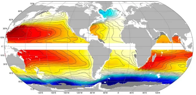
One of the main particularities of the large-scale ocean circulation is the so-called westward intensification, as shown in figure 1.1, where the flow lines tend to be close together over the western boundary, while they are spaced in the eastern boundary, illustrating that the flow is swift in the west, while it is sluggish on the opposite side of the basin. This feature characterizes all ocean basins and was first explained by Stommel (1948).

In that work, the author based his demonstration in simplified, theoretical models of the ocean and wind pattern, which consisted in a constant-depth rectangular ocean on one hemisphere, and a wind field only varying in the latitudinal direction, as show in figure 1.2. Stommel’s work exposed for the first time that the variation of the Corio-lis parameter with latitude is responsible for the western intensification of the currents in the ocean, and following works explained this feature in terms of vorticity conser-vation (e.g. Pond and Pickard, 1983; Rhines, 1986; Lozier and Riser, 1989). In general

(13)

1.2. The Humboldt Currents system

Figure 1.1: Mean absolute geostrohpic streamfunction at 5db from Argo data (2004-2010).

Contour interval is 100 m2s−1_{. Dark gray areas were ommited from the analysis. After Gray}

and Riser (2014).

terms, the vorticity put into the ocean by the wind stress must be taken out (or bal-anced) by friction. In the west, a strong friction is needed to balance out the vorticity acquired with the poleward increase in f, and for this strong friction to occur strong currents with strong shear are needed. As a result of the western intensification, we find slow currents with low lateral shear in the eastern side of the basin. This induces a poor ventilation of the circulation (Luyten et al., 1983) thus the “age” of the water masses found in the eastern ocean boundaries is higher compared with what is found in the western side (Fig. 1.3), as it is the case when comparing the eastern and western boundaries of the south Pacific.

1.2 The Humboldt Currents system

The south basin of the Pacific Ocean (60◦

S, 150◦

E-70◦

W) accounts for 25% of the total oceans volume, and hosts in its eastern boundary one of the four major coastal upwelling systems of the world. Named after the German naturalist Alexander von Humboldt, the Humboldt Currents System (HCS) extends from southern Chile (near 45◦_{S) to northern Peru (~4}◦_{S), and from the coast to ~90}◦_{W. This currents system is}

most notable for its prodigious production of small pelagic fish, which represents 27% of the current annual landing for the fisheries in the Pacific Ocean and has played a key role in the development of several countries for decades.

(14)

Figure 1.2: Flow patterns (streamlines) for a simplified wind-driven circulation model in the northern hemisphere with: (a) Constant Coriolis force, (b) Coriolis force increasing linearly with latitude. Idealized wind stress pattern used to force the model is also shown. After Stommel (1948).

1.2.1 Large scale circulation in the HCS

The large-scale oceanic circulation that shapes the HCS is closely related to the trade winds, which are dynamically set up in both the southern and northern hemispheres by the pressure gradient developed between a low pressure area near the equator and a high pressure region localized around 30◦

. This pressure gradient induces an air-flow from the mid-latitudes towards the equator, and creates a zonally-narrow wind convergence zone, known as the Intertropical Convergence Zone (ITCZ; Fig. 1.4). In the Pacific, the ITCZ is located on average around 10◦

N, although its position varies seasonally in connection with the easterlies. Another convection zone characteristic of the tropical Pacific is the South Pacific Convergence Zone (SPCZ), which corresponds to a low-level convection band associated with a subtropical maximum in cloudiness, precipitation and sea surface temperature (Kiladis et al., 1989). It extends from the southeast Pacific (30◦_S-120◦_{W) to Papua New Guinea, where it merges with the ITCZ}

(Fig. 1.4). Both the ITCZ and the SPCZ determine the large-scale mean rainfall pattern tropical Pacific band (Takahashi and Battisti, 2007a,b).

The variations of the wind system in the HCS are influenced by the latitudinal shifts of the ITCZ and trade winds in the northern hemisphere, and the latitudinal variations of the SPCZ (Karoly et al., 1998), but they are mainly driven by the shifts of the South Pacific High (SPH) present off central Chile (~30◦_{S). The changes in both the position}

and the intensity of the SPH impact the wind field in the HCS (Rutllant et al., 2004) and couple to the orographic effect of the Andean mountain range, which results in nearly alongshore equatorward winds close to the coast (Fig. 1.4).

(15)

Figure 1.3: Marine radiocarbon ages (relative to the atmosphere) at 18 and 187 m depth. After Fuente et al. (2015).

Figure 1.4: Mean sea level pressure (blue to orange contours) and wind magnitude and

direc-tion (arrows) in the south Pacific for the period 2000-2008 (ICOADS dataset). Black contours correspond to mean rainfall values of 3 and 6 mm day−1_{, evidencing the low-level convergence}

bands. Dashed red line qualitatively marks the mean position of the ITCZ.

HCS. Off Peru, the equatorward winds are intense and almost year-round, with a max-imum during austral winter (Bakun and Nelson, 1991; Dewitte et al., 2011). On the

(16)

other hand, the wind seasonal cycle off northern Chile peaks during austral spring (Blanco et al., 2002), and during austral summer off central/southern Chile (Garreaud and Muñoz, 2005), which has been related to the seasonal migration of the SPH (An-capichún and Garcés-Vargas, 2015). Off central Chile, the atmospheric conditions are also subject to the excitation of low atmospheric pressure systems that are trapped to the coast by the pressure gradient between the marine boundary layer and the coastal orography, and propagate polewards (Garreaud et al., 2002).

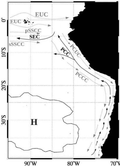
In the ocean, the circulation in the HCS is composed by several equatorward and poleward alternating currents, with a main surface equatorward flow north of 45◦

S (Strub et al., 1998) located next to the eastern rim of the SPH (Fig. 1.5). At around 10◦

S, the main flow turns offshore and flows into the South Equatorial Current (SEC), and a weak ramification continues equatorward and joins the SEC at around 8◦_{S (Wyrtki,}

1966). Below the surface, the ramifications of the eastward flowing Equatorial Under Current (EUC) nourish the subsurface poleward components of the HCS: (1) the Peru-Chile Under Current (PCUC), a subsurface poleward flow found over the slope and outer shelf off the Peruvian and Chilean coasts and (2) the Peru-Chile Counter Cur-rent (PCCC), located between 150 and 300 Km offshore (Strub et al., 1998; Fig. 1.5). In relationship with its equatorial origins, the PCUC has a distinctive hydrographic sig-nature, characterized as relatively saltier, higher in nutrients and lower in oxygen than the surrounding waters, and these characteristics have allowed to trace it as far south as 48◦_{S (Silva and Neshyba, 1979).}

The HCS exhibits an important seasonality in relation to the yearly cycle of the envi-ronmental forcing. On a regional scale, the oceanic response to envienvi-ronmental forcing at seasonal timescale is primarily related to the annual net insolation cycle (Takahashi, 2005), although ocean dynamics contribute to make the system heterogeneous and in-duce distinctive responses to forcing off Peru and Chile, which has been interpreted as the result of a compensation between large-scale dynamical signals (Dewitte et al., 2008a). On the other hand, the oceanic response to environmental forcing next to the coast is closely related to the wind forcing and manifests as coastal upwelling, which is the process responsible for the high primary productivity observed along the coast in the HCS. This coastal upwelling is sustained by the alongshore equatorward wind stress that generates an Ekman divergence of the currents next to the coast, which is in turn compensated by a vertical upward flow of nutrient-rich waters carried by the PCUC (Kelly and Blanco, 1984; Wyrtki, 1963). In addition, the large scale along-shore wind stress decreases over a few hundred kilometers next to the coast, due to the coastal orography, the surface drag gradient between land and sea, and the air-sea interactions over cool air-seawater (see Capet et al., 2004). It is expected that this

(17)

Figure 1.5: Oceanic circulation scheme in the HCS: Equatorial Undercurrent (EUC), primary

and secondary Southern Subsurface Countercurrents (pSSCC and sSSCC), South Equatorial Current (SEC), Peru Coastal Current (PCC), Chile Undercurrent (PCUC) and Peru-Chile Countercurrent (PCCC). Black lines denote surface currents and gray lines denote sub-surface currents. The average position of the 1020 mb sea level pressure contour (used as a proxy for the South Pacific High position) is also represented (H). Currents compiled following Strub et al. (1998), Kessler (2006) and Montes et al. (2010b).

phenomenon, also known as wind “drop-off”, would create an onshore wind stress gradient which would in turn result in a negative wind stress curl and ultimately an Ekman pumping (Bakun and Nelson, 1991) that could also contribute to the vertical upwelling.

Although the mechanisms behind the coastal upwelling in the HCS are related to the large scale wind system present in the region, the small scale variations in the ocean circulation and coastal orography contribute to make the system heterogeneous, encompassing three well-defined upwelling subsystems along the HCS (Montecino and Lange, 2009): (1) the year-round and highly productive upwelling system off Peru,

(18)

(2) a low productivity “upwelling shadow zone” in southern Peru and northern Chile, and (3) a productive and seasonal upwelling system in central-southern Chile.

1.2.2 The south Pacific Oxygen Minimum Zone

In addition to a highly productive upwelling system, the SEP encompasses the southern portion of one of the most extensive Oxygen Minimum Zones of the planet (OMZs; Paulmier and Ruiz-Pino, 2009). The OMZs are regions in the ocean character-ized by extremely low concentrations of Dissolved Oxygen (DO) in the water column (DO < 60 µM), as a result of complex interactions between the ocean circulation and the biogeochemical cycles (Fig. 1.6; Karstensen et al., 2008). In the HCS, the intense biological production that takes place in the euphotic zone of the water column (first 200m) is accompanied by an important subsurface remineralization of organic matter, which translates as a significant DO demand in the mesopelagic zone (Capone and Hutchins, 2013). This important DO demand couples to poor ventilation, related to a nearly stagnant circulation (Luyten et al., 1983), which allows the OMZ to persist in time. Among the most relevant impacts of the OMZ in the SEP we find the habi-tat compression of the organisms, given that the OMZ represents a respiratory barrier (Prince and Goodyear, 2006). Additionally, the biogeochemical cycles that take place at extremely low DO concentrations are involved in the local production of climatically-active gases, such as CO2(Paulmier et al., 2011) and N2O (Kock et al., 2016), which are

then outgassed to the atmosphere. In this sense, the OMZ has an impact on both the local ecosystems and on the global climate.

Despite its potential implications, several questions remain regarding the OMZ variability and long-term trends (Stramma et al., 2010). Recent light has been shed upon the mechanisms that shape the OMZ (Bettencourt et al., 2015), emphasizing the central role of the mesoscale structures. However, it has not been clarified yet whether or not these structures influence the variability of the OMZ and its long-term evolu-tion, considering that the mesoscale activity appears as a conspicuous feature in the SEP circulation.

1.2.3 Mesoscale features

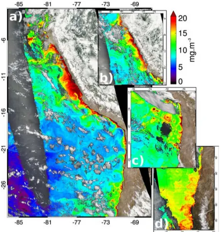
Over the large-scale circulation pattern found in the HCS, rich mesoscale variabil-ity in the form of eddies or vortices, filaments and squirts is superimposed (Fig. 1.7). In the HCS, eddies are characterized by a radius between 50-150 km (Chaigneau et al., 2008; Chaigneau and Pizarro, 2005b) and can persist for months, traveling thou-sands of kilometers offshore from their genesis region. Eddies are mainly generated

(19)

Figure 1.6:Global Oxygen Minimum Zones (OMZ), including the upper depth of intermediate

water hypoxia (DO < 60 µmol L−₁

; color shading), and the spatial distribution of severely hypoxic minimums (DO < 20 µmol L−₁

) as white lines. After Moffitt et al. (2015).

from baroclinic instabilities induced by the vertical shear of the currents near the coast (Leth and Shaffer, 2001), and propagate westward with translation velocities between 3-7 cm s−₁

(Chaigneau and Pizarro, 2005b). Observations have shown that the HCS is highly populated by eddies between 9◦_{S and ~36}◦_{S, and they participate in the heat}

(Colas et al., 2012) and salt balance between the offshore and coastal waters through lat-eral fluxes, even exceeding the mean advective current fluxes in the coastal upwelling region (Chaigneau and Pizarro, 2005a). Despite this evidence, the net contribution of eddies to the SEP’s heat budget is still in debate, due to conflicting modeling and obser-vational results (cf. Mechoso et al., 2014). Recent obserobser-vational analyses even suggest that eddies would not substantially contribute to the surface layer heat budget in the offshore SEP (Holte et al., 2013).

In the SEP, the mesoscale structures also induce a coupling between physical and biogeochemical processes (McGillicuddy et al., 1998), which significantly extends the high primary production zone associated to the coastal upwelling while moving off-shore. Observational evidence off central Chile (29◦_-39◦_{S) indicates that eddies are}

responsible for more than 50% of the winter chlorophyll-a peak in the offshore coastal transition zone (Correa-Ramirez et al., 2007). In this sense, eddies might represent a pathway that links the highly productive coastal upwelling region with the (essentially

(20)

oligotrophic) offshore waters. Nevertheless, this vision is still on debate regarding the highly productive HCS and recent results have established that in fact eddies might contribute to reduce primary productivity as a result of the transport of nutrients from the nearshore to the open ocean (Gruber et al., 2011)

1.3 Teleconnection with the equatorial Pacific

Aside from the local atmospheric and oceanic forcing, the variability in the HCS is intimately related to the variability that takes place in the equatorial Pacific, at timescales ranging from intraseasonal to seasonal (Pizarro et al., 2002; Shaffer et al., 1999), and from interannual (Pizarro et al., 2001, 2002; Vega et al., 2003) to interdecadal (Monte-cinos et al., 2007). The equatorial region behaves as a waveguide, and allows for the

Figure 1.7: Chlorophyll-a concentration in the Humboldt currents system, illustrating the

rich mesoscale variability that is present in the flow. Structures such as eddies, filaments and plumes can be clearly distinguished. The chlorophyll-a data corresponds to snapshots taken by the MODIS spectroradiometer (1 km resolution) at different dates: (a) 18/02/2014, (b) 17/01/2014, (c) 13/09/2014 and (d) 06/07/2014. The coastal orography and clouds correspond to corrected reflectance (true color), also acquired by MODIS. Data source: http://worldview.earthdata.nasa.gov

(21)

1.3. Teleconnection with the equatorial Pacific

zonal propagation of different types of waves. One of the most prominent modes of variability corresponds to the Intraseasonal Equatorial Kelvin Wave (IEKW), gener-ated in the central equatorial Pacific by intraseasonal westerly wind pulses. The IEKW travels to the east and impinges on the American continent. As shown by idealized models, part of the energy is reflected by the eastern boundary and travels to the west as a long Rossby wave, and part is deflected and travels poleward (Cane and Sarachik, 1977; Moore and Philander, 1977) as a free Coastal Trapped Wave (CTW). The South American coast behaves then as an extension of the equatorial waveguide. In contrast to the IEKW, the phase speed of the CTW strongly depends on the shape of the con-tinental slope (Brink, 1982; Clarke and Ahmed, 1999) and stratification (Allen, 1975), and its vertical structure varies with latitude. As the wave travels polewards, the inter-nal Rossby radius of deformation decreases and the bottom topography becomes more important in determining the vertical structure of the gravest baroclinic modes (Brink, 1980). In this manner, at low latitudes the CTW structure is essentially baroclinic, how-ever, as latitude increases, the dominant vertical structure tends to be barotropic (Brink, 1982).

As they travel polewards, the CTWs induce perturbations in the density and pres-sure field over the continental shelf and slope, which has permitted to observe pole-ward propagating signals along the South American coast at a wide range of frequen-cies. Fluctuations of sea level and currents off Peru in the synoptic band (period ~10 days) have been reported to have little relationship with the local wind (Cornejo-Rodriguez and Enfield, 1987; Enfield et al., 1987; R. L. Smith, 1978). Rather, they re-late to the poleward propagation of first baroclinic mode CTWs (Brink, 1982; Romea and R. L. Smith, 1983), forced by synoptic-scale mixed Rossby-gravity waves (or Yanai waves), propagating eastward in the equatorial Pacific (Clarke, 1983; Enfield et al., 1987). Further studies unveiled the relationship between the sea level and currents fluctuations observed in the HCS at intraseasonal frequencies (30-90 days) and the re-mote influence through first baroclinic mode CTWs (Hormazábal et al., 2002; Illig et al., 2014; Shaffer et al., 1997; Spillane et al., 1987), forced by baroclinic IEKWs impinging on the South American coast. Such wind-forced equatorial waves tend to be most promi-nent during austral summer in the central tropical Pacific (Illig et al., 2014; Kessler et al., 1995), in connection with atmospheric convection events that propagate from the central Indian Ocean into the western Pacific.

The IEKW activity is strongly modulated at interannual timescales reflecting the occurrence of El Niño events (Dewitte et al., 2008a; Kessler et al., 1995) and its diversity (Gushchina and Dewitte, 2012; Mosquera-Vásquez et al., 2014), which corresponds to the most prominent mode of climatic variability in the equatorial Pacific.

(22)

1.3.1 A brief description of El Niño

The occurrence of El Niño events entails important disruptions in the tropical Pa-cific climate system primarily associated with changes in the SST gradients and the ocean-atmosphere feedbacks. Due to the efficient teleconnection that links the trop-ical Pacific and the SEP, this mode of troptrop-ical climatic variability induces significant upheavals in the SEP climate system, which highlights the fact that the influence of these events extends well beyond the equatorial Pacific. In the present section, a brief description of El Niño is made, and the modulation of the SEP variability induced by these events is presented in the following section.

AVERAGE CONDITIONS: in the tropical Pacific, the wind regime dominated by

the easterlies induces a flow to the western part of the basin. As the water flows westwards along the equatorial region, the strong insolation induces a surface warming, and a strong zonal SST gradient is developed (around 12◦_{C between}

the western and eastern Pacific). This zonal gradient reflects as a tongue-shaped cold Sea Surface Temperature (SST) that extends from east to west, and a deeper equatorial thermocline develops in the western Pacific (Fig. 1.8a). The warm water found in the western boundary (known as the “warm pool”) generates an important atmospheric thermal convection. The warm and humid air over the warm pool ascends and is driven by the high tropospheric circulation towards the eastern part of the basin, where it loses heat and humidity and settles above the colder sea surface. The air is then driven towards the west by the easter-lies, closing the convective loop. This atmospheric circulation cell is known as the Walker circulation (Fig. 1.8a), in honor of Sir Gilbert Walker, who first de-scribed the strong inverse correlation between the high and low pressure records obtained at the eastern and western Pacific, and coined the term Southern Oscil-lation to describe the “seesaw” behavior of the east-west pressure gradient. EL NIÑO EVENTS: the onset of an El Niño event is characterized by a relaxation

of the easterlies, and a consequent reduction of the equatorial and coastal up-welling, which allows the warm pool to grow and expand eastward in the equa-torial Pacific (Fig. 1.8b). The shift of the warm pool position induces a zonal displacement of the convective Walker cell which in turns changes the evapora-tion patterns, generating droughts in the western part of the basin, and strong precipitations in the eastern part (Fig. 1.8b). These events might be followed by cold events in the central equatorial Pacific, known as La Niña events (Fig. 1.8c), which are considered as an enhancement of the average conditions. Dur-ing a La Niña event, the easterlies are stronger than the average conditions, the

(23)

Figure 1.8: (a) Normal conditions in the tropical Pacific. Conditions during (b) an El Niño

event and (c) La Niña event. After Ashok and Yamagata (2009).

warm pool is warmer than average and the waters in the eastern Pacific are even colder (Fig. 1.8c), which couples to a stronger-than-average Walker circulation. This marked ocean/atmosphere coupling between the anomalies generated by El Niño events and the Southern Oscillation is referred to as El Niño-Southern Oscillation (ENSO).

1.3.2 The ENSO arrival at the Humboldt Currents System

Although the ENSO events peak in the equatorial Pacific, wave dynamics carry the anomalous ENSO signal to the SEP. The equatorial Pacific is heavily disrupted dur-ing ENSO events, and this reflects on the IEKW activity. Kessler et al. (1995) showed that during the onset of El Niño events, the eastward extension of the convection cell (associated with a warmer SST) gives the westerlies more fetch to blow upon, gener-ating a more intense IEKW activity. This is coupled to a deepening of the thermocline along the equatorial Pacific, which favors the leading baroclinic mode and enhances the phase speed of the IEKW (Benestad et al., 2002). These changes translate as a mod-ulation of the IEKW at interannual timescale (Dewitte et al., 2008a), which ultimately impacts the CTW activity in the HCS (Enfield et al., 1987). In this sense, Shaffer et al. (1997) documented the intraseasonal currents variations at central Chile (30◦_S)

dur-ing the 1991-1992 El Niño event, showdur-ing that the most important fluctuations were related to the passage of free CTWs arriving from the north.

Additionally, the CTW activity during the ENSO events severely impacts the coastal thermocline. At the peak of the 1997-1998 El Niño, the thermocline off the coasts of southern Peru and northern Chile showed vertical anomalies in the order of 150m, which were perceived as anomalies in the order of 10 cm in the coastal sea levels ob-servations (Blanco et al., 2002). Several studies evoked the idea that the vertical dis-ruptions of the thermocline depth forced by the intraseasonal CTWs would have an

(24)

impact on the source water for the coastal upwelling, such that the upwelled water would be cooler or warmer (and nutrient rich/poorer), in relationship with the up-welling/downwelling phase of the wave (Colas et al., 2008; Huyer et al., 1987; Shaffer et al., 1997). This relationship has been recalled, together with the variations in the alongshore wind intensity (Rutllant et al., 2004), to explain the low productivity ob-served in the HCS during El Niño events (Barber and Chávez, 1986; Huyer et al., 1987), and the subsequent drop of the fisheries (86% decrease during the 1997/98 El Niño; see Yañez et al. (2001)).

1.3.3 The connection between the equatorial Pacific and the deep

eastern Pacific

The oceanic teleconnection between the eastern and equatorial Pacific is not lim-ited to the propagation of CTWs. Theoretical works first showed that, depending on the frequency, the motion might be not only in the form of a Kelvin-like wave trapped along the meridional boundary, but also in the form of long Rossby waves, with a group velocity away from the boundary (Clarke, 1983; Schopf et al., 1981). Further studies demonstrated that for a given frequency, there is a critical latitude (or distance from the equator) such that the energy radiates offshore in the form of baroclinic Extra-Tropical Rossby Waves (ETRW) equatorward of that critical latitude (Clarke and Shi, 1991). The formalism that relates frequency and latitude establishes that lower fre-quencies favor the untrapped motion, and therefore ETRW can radiate at any latitude along the coast for interannual timescales (Schopf et al., 1981), which has been corrob-orated by observations as far from the equator as 30◦_{S (Fig. 1.9).}

The offshore radiation of energy in subtropical latitudes at interannual timescales was first evidenced for the north Pacific (Kessler, 1990; White and Saur, 1983), us-ing observations of the subsurface thermal structure. Nonetheless, the lack of a well-established observation system (as the one present in the equatorial Pacific) held back a more detailed characterization of the ETRW, as well as their modulation and inter-actions with the mean circulation. This issue was partly addressed with the first long term observations resulting from the altimetric TOPEX/Poseidon mission, which re-vealed that the ocean is populated by an ubiquitous Rossby wave field (Chelton and Schlax, 1996), that has the potential to modulate the average circulation in the ocean. In this matter, Qiu (2002) analyzed eight years of the (then) recent altimetric mission to investigate the interannual changes in three subtropical current systems in the north Pacific. This unprecedented work revealed that much of the interannual perturbations observed in the large scale circulation in the mid-latitude system were related to sea

(25)

surface height (SSH) anomalies, that propagate from the eastern boundary toward the basin interior as baroclinic long Rossby waves.

First observations also documented a decrease of the ETRW amplitude as they propagate westward (Chelton and Schlax, 1996; Wang et al., 1998), and several mech-anisms were evoked to explain it. Qiu et al. (1997) proposed a theoretical framework that evaluated the westward decay of long baroclinic Rossby waves off the equatorial region, related to the effect of eddy dissipation. Later on, using a quasigeostrophic two-layer model, Lacasce and Pedlosky (2004) also recall the nonlinearities of the flow as the source of dissipation, explaining the dissipation process in terms of the baro-clinic instability of the Rossby wave itself. In that work, the authors propose that the growth of baroclinic instability of the wave may overcome the stabilizing effect of the planetary vorticity gradient (β effect), and cause the wave to breakdown and transfer energy to a smaller-scale eddy field. Yet, the linear dispersion of Rossby waves associ-ated with the β effect also constitutes a type of dissipation. Schopf et al. (1981) showed that linear dispersion generates a caustic line that originates at the critical latitude and defines a limit for the propagation of boundary forced Rossby waves. Given that linear dispersion becomes increasingly important away from the equator, it is also a potential mechanism that could explain the observed surface decay of the ETRW away from the boundary.

An additional process to consider in the interpretation of the surface signature of long Rossby waves is the vertical propagation of energy that involves the constructive contribution of a certain number of baroclinic modes (Gent and Luyten, 1985; Mc-Creary, 1984). Vertical propagation of long Rossby waves was first investigated in the

Figure 1.9: Longitude-time diagrams of interannual sea level anomalies (TOPEX/ERS dataset)

for the second half of the 1990s, at three latitudes along the HCS. In particular, the westward propagation a downwelling ETRW, associated with a strong positive sea level anomaly near the coast(> 6cm), can be distinguished for the 1997/1998 El Niño event. After Vega et al. (2003).

(26)

equatorial region, in order to document and explain the variations of temperature ob-served below the thermocline at annual period (Kessler and McCreary, 1993). Using an ocean general circulation model (OGCM), Dewitte and Reverdin (2000) successfully reproduced Kessler and McCreary’s results in terms of annual subthermocline variabil-ity, and reported that the vertical energy propagation in the form of long Rossby waves also takes place at interannual timescale, associated with the reflection of Kelvin waves on the eastern boundary of the equatorial Pacific basin (which are prominent during strong El Niño events).

Figure 1.10: Cross-shore sections of

vertical isotherms displacements (in meters) during the peak phase of the 1997/1998 El Niño event at 15◦

S (top), 20◦

S (middle) and 30◦

S (bot-tom). After Ramos et al. (2008).

In the SEP, works focusing on the variability of the vertical structure of the circulation later documented the existence of vertical propagation of ETRW at seasonal (Dewitte et al., 2008b) and interannual (Ramos et al., 2008) timescales, evi-dencing a vertical energy flux associated with the propagation of the ETRW. In particular, Ramos et al. (2008) illustrated the close connection be-tween the subthermocline variability in the SEP and the equatorial variability during the 1997-1998 El Niño event. As the event develops, high-order baroclinic mode contribution to the equato-rial Kelvin wave becomes more important, related to a change in the equatorial thermocline depth and vertical temperature gradients (Dewitte et al., 2003). This translates as an increasing dom-inance of high baroclinic modes along the coast in the SEP throughout the event, which construc-tively trigger the vertical propagation of ETRW. As shown by Ramos et al. (2008), the signature of the ETRW related to the ENSO events extends sev-eral hundreds of Km offshore and penetrates deep into the ocean (Fig. 1.10), which questions about the role that the vertical energy propagation re-lated to the ENSO events could play in the venti-lation of the subsurface circuventi-lation in the SEP. This acquires particular relevance in the current under-standing of the ENSO diversity and its influence out of the tropical Pacific.

(27)

1.4. ENSO diversity

1.4 ENSO diversity

Recent studies have reported that over the last five decades, two types of El Niño events have occurred in the equatorial Pacific (Ashok et al., 2007; Kug et al., 2010; Larkin and Harrison, 2005; Yeh et al., 2009), each one having contrasting SST anomaly patterns: (1) the Cold Tongue El Niño, or eastern Pacific El Niño (Fig. 1.8b), consist-ing in a SST anomaly that develops and peaks in the eastern equatorial Pacific (EP), and the (2) El Niño Modoki (Ashok et al., 2007) or central Pacific El Niño (CP), that consists of an SST anomaly that develops and persists in the central equatorial Pacific (Fig. 1.11). In addition, both types also differ in the intensity of the SST anomalies de-veloped in the tropical Pacific, with the stronger events occurring in the eastern Pacific (EP). They also exhibit different seasonal evolution patterns (Kao and Yu, 2009; Yeh et al., 2014). During the EP events, the SST anomalies develop in the far eastern Pacific during boreal spring and extend westward over summer and fall, while during the CP events, the SST anomalies extend from the eastern subtropics to the central equatorial Pacific during boreal spring and summer. Despite the phase differences during the development phase, both event types achieve their peak amplitude in boreal winter.

Figure 1.11: Conditions in the tropical Pacific during a central Pacific El Niño event. After Ashok and Yamagata (2009).

The contrasting characteristics of both types of El Niño imply different impacts as-sociated with their occurrence. Each type induces a different zonal SST gradient across the equatorial Pacific, and this translates as contrasting atmospheric teleconnections (Ashok et al., 2007; Weng et al., 2009; Yeh et al., 2009). While the convective cell is displaced far to the east during the EP events, the SST anomalies developed during the CP events induce an anomalous twin Walker circulation, with the updraft branch located in the central Pacific (Fig. 1.11; Ashok et al., 2007). Significant differences are also observed in the HCS related to each type of El Niño. While EP events are associ-ated with drastic changes in coastal circulation and hydrographic conditions (Fig. 1.12;

(28)

Blanco et al., 2002; Pizarro et al., 2001) and therefore have a profound impact on the local ecosystems (Gutiérrez et al., 2008), the changes imposed by the CP events on the hydrographic characteristics of the HCS are not as severe as during EP events, and are in turn very close to the climatological mean (Fig. 1.13; Dewitte et al., 2012). Recent studies also show that the IEKW activity is distinct between CP and EP El Niño events (Gushchina and Dewitte, 2012; Mosquera-Vásquez et al., 2014).

Figure 1.12: (a) Time-latitude plot of monthly sea level height interannual anomalies from tide gauge data along the coast of the HCS, from 1980 to 1998. (b) time-depth plot of temperatures 10 km offshore of Iquique (20◦

S). Note the severe thermocline depression during the 1981/1982 and 1997/1998 El Niño events. Sampling is indicated by arrows. After Blanco et al., 2002.

1.4.1 ENSO diversity trend

Observations point out that the ENSO diversity has accentuated over the last part of the 20th century (Fig. 1.14). CP events have become more frequent (Lee and McPhaden,

(29)

1.5. Thesis motivations and objectives

Figure 1.13: Composites of the mean thermocline depth off the coast of Peru during the peak

(DJF) and decaying (MAM) phase of an eastern (thick) and central (thick dotted) Pacific El Niño event. The thin line correponds to the average thermocline depth over the period 1958-2007. After Dewitte et al. (2012).

2010) as compared to prior decades, which has been interpreted as being related to changes in ENSO characteristics due to global warming (Yeh et al., 2009). Indeed, SST projections in CMIP-class models predict an increase in the ratio of CP type to EP type under different global warming scenarios (Kim and Yu, 2012; Yeh et al., 2009), which is associated with changes in the atmospheric circulation over the tropical Pacific (Vecchi et al., 2006; S.-P. Xie et al., 2010). However, the real impact of global warming on the ENSO diversity is difficult to assess, given that this diversity might also be intrinsically forced by natural variability of the climate system. Using random combinations of spatial structures obtained by a linear stochastic model, Newman et al. (2011) showed that extended epochs dominated by either EP or CP events can be reproduced even when excluding the anthropogenically-induced changes in the background state. Such spontaneous generation of multidecadal epochs of CP and EP events has also been re-produced in coupled GCMs (Kug et al., 2010; Wittenberg et al., 2014), which challenges the interpretation of the ENSO diversity as being a forced mode of variability related to the anthropogenic influence on global warming.

1.5 Thesis motivations and objectives

One of the major concerns in the climatic and oceanographic community is the current earth’s energy imbalance (EEI), which arises from an imperfect closure of the

(30)

Figure 1.14: Intensity of El Niño events in the central (left panel) and eastern (right panel) Pacific. Linear trend corresponds to 0.20(±0.18)◦

C/decade in the central Pacific and 0.39(±0.71)◦

C/decade in the eastern Pacific. After Lee and McPhaden, 2010.

planetary radiative budget and manifests as a radiative flux imbalance between the in-coming and outgoing radiation in the top of the atmosphere (Hansen et al., 2011). Cur-rently, EEI is positive and is evidenced as a global rise in temperature and sea level, acceleration of the hydrological cycle and increase in the ocean heat content (OHC). Although many aspects of climate are determined by the heat capacity of all the com-ponents of the climate system (atmosphere, land, ice and ocean; Trenberth and Stepa-niak, 2004), most of the energy accumulation from the EEI manifests as an increased OHC (Abraham et al., 2013; Church et al., 2011), and even though recent evidence shows that the largest fraction of OHC increase has occurred in the upper 700m, both observational and modeling studies indicate that ~25% of OHC increase over the last 45 years took place between 700-2000m depth (Balmaseda et al., 2013; Levitus et al., 2012; Purkey and Johnson, 2010) and indirect estimations for the full-depth OHC are in good agreement with the estimated total EEI (Llovel et al., 2014). This highlights the potential role of the intermediate-deep ocean in buffering the EEI, and calls for a bet-ter understanding of the mechanisms that participate in the “ventilation” of the deep oceanic circulation. In this context, the vertical propagation of ETRW that takes place in the SEP, which constitutes a mechanism that links the shallow coastal ocean with the deep offshore and conveys information about the tropical surface variability, has the potential to participate in the oceanic response to the EEI.

While the coastal circulation and its variability in the SEP are relatively well doc-umented, little is known about the variability of the mid-depth and deep circulation components of the system. Observations have shown that currents in the meso and abyssopelagic regions present a marked seasonal cycle, as well as an interannual mod-ulation (Shaffer et al., 2004), which has been interpreted as related to Rossby waves

(31)

emanating from the coast in connection with ENSO events. Nevertheless, little has been said about the long-term variations of this mechanism, in connection with the decadal changes observed in the tropical Pacific. No information about a possible im-pact of the ETRW on the deep ocean other than a modulation of the currents has been brought to light either. This last point is of particular importance, considering the near stagnant nature of the mean circulation in the SEP.

One of the major difficulties in documenting the changes in the SEP circulation is imposed by the lack of a systematic observational system, and particularly in the subsurface, where in situ observations are practically nonexistent. International efforts aiming to resolve this issue are currently underway, such as the deployment of floats in the context of the ARGO program, but the spatial and temporal resolution in the SEP is to the present day very low (Fig. 1.15).

Figure 1.15: Argo floats sparseness in the south Pacific ocean (as to 21/04/2016). Distance

corresponds to the average distance to the 4 nearest floats. Source: http://argo.whoi.edu

(32)

from the current generation of global general circulation models; however, the spa-tial resolution that is implemented in the global products generates important misrep-resentations of both the oceanic and atmospheric circulation patterns near the coast (Richter, 2015; Zheng et al., 2011), which induces severe biases in the coupled simu-lations, and particularly in the upwelling regions (Fig. 1.16) where important warm biases are observed. In addition, uncertainties in the atmospheric and oceanic reanal-ysis products used to force the OGCMs also constitute a source of errors, which has been evoked to interpret the biases observed in forced ocean simulations (e.g. Brodeau et al., 2010). In particular, the accuracy oceanic reanalysis products is penalized by the lack of in situ observations available to constrain the assimilation process, which are practically nonexistant in some regions (see Lee and McPhaden (2010) for a review), and atmospheric reanalysis also present errors that are relevant for the dynamics of coastal systems (e.g. wind stress divergence close to the coast (Astudillo et al., 2016); errors in air-sea fluxes (Chaudhuri et al., 2013)). A suitable answer to overcome some of these difficulties could be the use of a regional ocean-modeling platform. The high-resolution capability of this tool greatly improves the biases observed in coastal up-welling systems using global models (e.g. Colas et al., 2012; Dewitte et al., 2012; Pen-ven et al., 2001), and provides with reliable long-term simulations of three-dimensional ocean fields.

In this context, several questions arise regarding the variability of the SEP, which motivates the present work:

• One of the main motivations for the present work is to better understand the sea-sonal to interannual variability of the deep ocean (subthermocline) in the SEP, with a focus on its forcing mechanisms and how this relates with the elements encompassed by the subthermocline circulation in the SEP. In particular, the im-plications that the variability of the circulation in this region have for the un-derstanding of the OMZ dynamics is a current concern for the community and remains unaddressed.

• As previously discussed, the ocean plays a central role in the planetary energy budget at climatic scale, which is reflected by the variations in the OHC. The correct interpretation of the current OHC trends (and the EEI trends) therefore requires a sound understanding of the ocean’s ability to store and vertically re-distribute the excess of energy, which is naturally limited by our knowledge on the processes involved in the deep circulation variability. In this sense, improv-ing the current understandimprov-ing of a process that could have implications for the ocean’s role at climatic scale, such as the vertical propagation of ETRW, is also a motivation for the present work.

(33)

Figure 1.16: (a) Observed annual mean sea surface temperature (SST) from the optimally

in-terpolated (OI) SST data set. (b) Annual mean bias of the CMIP5 ensemble, relative to OISST. Gray boxes denote the four upwelling regions, where the biases are particularly important. Af-ter RichAf-ter (2015).

1.5.1 Scientific objectives and manuscript plan

Although there is substantial evidence that supports the propagation of extra tropi-cal Rossby waves as being a prominent component of the SEP circulation variability at different timescales, this process has not been appropriately diagnosed yet. The main goal of this thesis work is thus to document the connection between the variability that takes place in the equatorial Pacific and the variability of the subsurface circula-tion along the coasts of Peru and Chile. Within this context, we can summarize the objectives and the approach of the present work as follows:

(34)

• To document the vertical energy flux associated with the propagation of the extra-tropical Rossby wave.

• To investigate the influence of the ETRW on the variability of the OMZ.

• The flow fluctuations in the form of mesoscale structures, prominent in the re-gion, should also influence the variability of the circulation in the SEP. To evalu-ate the influence of the mesoscale activity on the variability of the OMZ, and on the energy flux related to the ETRW are complementary objectives of the present work.

In order to answer to the scientific questions and achieve the objectives previously outlined, the thesis manuscript is organized as follows: Chapter 2 introduces the tools and methodological approach used to study the variability of the circulation in the SEP and briefly presents the formalism that supports the vertical propagation of extra-tropical Rossby waves. Chapter 3 focuses on the study of the vertical energy flux re-lated to the propagation of the extra-tropical Rossby wave at interannual to decadal timescales, and how it is impacted by the mesoscale activity. Chapter 4 addresses the impact that the fluctuations of the circulation in the form of ETRW and mesoscale pro-cesses have for the ventilation of the HCS, from the perspective of the OMZ ventilation at seasonal timescale. Finally, Chapter5 presents the conclusions of the present work and proposes some future perspectives around the study of the subsurface circulation in the region.

(35)

Introduction (français)

Situé le long des côtes du Pérou et du Chili, le Système de Courant de Humbolt (HCS5_{) est l’un des plus grand systèmes d’upwelling du monde, reconnu notamment}

pour sa forte productivité en termes de ressources halieutiques. Ce système de courant est sujet à une riche variabilité induite par les interactions océan-atmosphère ayant lieu tout le long de la côte. Sa variabilité est également modulée par l’influence à distance de la variabilité présente dans le Pacifique équatorial, et qui se propage le long de la côte Sud-Américaine.

La circulation grande échelle du Pacifique s’organise autour d’un système de haute pression, l’Anticyclone du Pacifique Sud (SPA6_{). Cet anticyclone influence les}

princi-pales caractéristiques de la circulation moyenne dans le Pacifique Sud, dont l’asymétrie Est-Ouest que l’on retrouve dans tous les basins océaniques. Cette asymétrie consiste en des courants très forts vers les pôles coulant le long des façades Ouest des océans, et qui contrastent avec les courants des bords Est, beaucoup moins énergétiques, ce qui entraine de faibles taux de ventilation de la circulation.

Localement, la circulation dans le HCS est fortement liée au vent qui souffle en surface le long des côtes Sud Américaines en direction de l’équateur. Ce vent influ-ence d’une part la circulation moyenne de surface que l’on observe dans la région, dirigée comme le vent vers l’équateur, et d’autre part, le vent parrallèle à la côte induit un transport des eaux de surfaces vers le large, remplacées par des eaux profondes, froides, riches en nutriments et en gaz carbonique. Cette dynamique permet la fertilisa-tion des couches de surfaces sur le plateau continental, ce qui déclenche des maximums locaux de productivité primaire caractéristiques de la région. Bien que l’upwelling soit la principale caractéristique régionale, son intensité varie le long de la côte en fonction de l’orographie locale et de l’intensité du vent. On peut ainsi observer différentes sous-régions : (1) le Pérou, avec un système d’upwelling très productif et quasi-permanent, (2) un système très peu productif entre la frontière Sud du Pérou et le Nord du Chili, et (3) un système très productif et marqué par des variations saisonnières le long des côtes du Chili central et Sud.

En plus de ces systèmes d’upwelling, le HCS abrite la partie sud de la Zone de Mini-mum d’Oxygène (OMZ7_{) la plus étendue au monde. Cette OMZ résulte de l’interaction}

entre les forts taux de production primaire ayant lieu dans la couche euphotique, la dégradation de la matière organique produite consommant de l’oxygène, et de la circu-lation lente et peu énergétique présente sous la surface, ce qui favorise l’accumucircu-lation

5_{De l’anglais Humbolt Currrent System.} 6_{De l’anglais South Pacific Anticyclone.} 7_{De l’anglais Oxygen Minimum Zone.}

(36)

des eaux pauvres en oxygène.

Malgré leur diversité, les impacts de l’OMZ ont été jusqu’à présent relativement peu étudiés. En effet, l’OMZ du Pacifique Sud est impliquée dans la libération de gaz à effet de serre, notamment le N2O et le CO2, qui sont importants à prendre en

compte en termes de climat global. De plus, cette zone réduit l’espace habitable par les organismes marins à cause des faibles concentrations en oxygène, ce qui impacte les ressources halieutiques de la région. Ces conséquences peuvent être significatives, et ce à différents niveaux, mais l’étude de la dynamique de l’OMZ en est encore au stade initial. Par exemple, il a récemment été mis en évidence que l’activité méso-échelle régionale serait le facteur principal de la forme et de l’étendue de l’OMZ. Cependant, l‘impact de l’activité méso-échelle sur la variabilité de l’OMZ n’a pas encore été étudié. On peut donc s’interroger sur l’effet que la variabilité interne de l’océan pourrait avoir sur les tendances à long terme de l’OMZ.

Les structures de méso-échelle, dominantes dans la région, résultent des instabilités de la circulation, principalement du cisaillement vertical des courants. Les tourbillons de méso-échelle se propagent vers l’Ouest et participent ainsi au bilan de chaleur et de sel entre la zone côtière et le large. Ces structures participent également au couplage physique/biogéochimique qui étend la région fortement productive de la côte vers le large.

En plus du forçage atmosphérique local et de la variabilité interne, la modulation de la circulation du HCS est fortement liée à la variabilité d’origine équatoriale, à des échelles de temps allant de l’intra-saisonnier au décennal. La côte Sud-Américaine agit comme une extension du guide d’ondes équatorial, permettant ainsi la propagation des ondes de type Kelvin piégées à la côte (CTW8_{) vers le pôle. La propagation de}

ces signaux d’origine équatoriale le long des côtes du HCS entraîne la modulation des caractéristiques océanographiques du plateau continental jusqu’au talus, qui se manifestent sous la forme de perturbations sur les champs de densité et pression, en particulier à l’échelle de temps intra-saisonnière.

L’activité des CTW est particulièrement intense pendant les évènements El Niño (ENSO9_{), qui est relié à une activité plus importante des ondes de Kelvin à l’équateur.}

Ce mécanisme transmet l’information depuis le Pacifique équatorial vers le HCS, et est responsable des fortes anomalies dans les caractéristiques océanographiques enreg-istrées le long des côtes Sud-Américaines pendant les évènements ENSO. Par exem-ple, au cours de la période d’intensité maximale de El Niño 1997-1998, la thermocline s’approfondît de plusieurs dizaines de mètres (∼150 m) du côté Est du Pacifique en réponse au passage des CTW, ce qui était également observé sur le niveau de la mer à

8_{De l’anglais Coastal Trapped Waves.} 9_{De l’anglais El Niño Southern Oscillation.}

(37)

la côte, avec des anomalies de l’ordre de la dizaine de centimètres. Plusieurs travaux ont évoqués l’idée que les déplacements verticaux de la thermocline, forcés par le pas-sage des CTW au cours de l’ENSO de 1997-1998, pourraient modifier la source des eaux de l’upwelling selon la phase de l’onde (“upwelling” ou “downwelling”). Ce mécanisme, associé aussi aux variations du vent parallèle à la côte, serait à l’origine des chutes des taux de production primaires observés pendant cet évènement, qui ont eu des conséquences catastrophiques sur les ressources halieutiques et leur exploita-tion dans cette région.

Aux échelles interannuelles, l’influence du Pacifique équatorial sur le HCS n’est pas confinée à la côte, et s’étend également vers le large grâce à la propagation d’ondes de Rossby extratropicales (ETRW10_{). Les premières observations de la propagation de}

ce type de signal hors des latitudes tropicales ont été apportées par l’altimétrie, avec la mission TOPEX/Poséidon. Ce type d’observations a donné accès, pour la première fois, à un champ quasi simultané du niveau de la mer global, permettant de docu-menter également la propagation des signaux se dirigeant vers l’Ouest depuis la côte Sud-Américaine, associés à l’évènement El Niño 1997-1998.

Les observations altimétriques mettent aussi en évidence la décroissance significa-tive de l’amplitude de l’ETRW lors de sa propagation vers le large. Ceci peut être lié à différents mécanismes, par exemple, la dissipation turbulente, le “déferlement” de l’onde lié aux instabilités de type barocline, ou encore la dispersion linéaire. La prop-agation d’énergie verticale induite par la contribution d’un certain nombre de modes baroclines est un autre mécanisme qui peut aussi expliquer l’atténuation de l’onde de Rossby vers le large. Ce type de mécanisme a été étudié dans un premier temps pour expliquer les variations des températures de subsurface observées dans le Paci-fique équatorial à l’échelle annuelle, et a été généralisé par la suite pour les variations aux fréquences interannuelles, liées aux variations induites par le phénomène El Niño. Des travaux postérieurs ont mis en évidence que ce processus n’est pas exclusif au Paci-fique équatorial, mais que la propagation verticale d’énergie liée à l’onde de Rossby est aussi présente dans le Pacifique Sud-Est. En particulier, Ramos et al. (2008) met en év-idence la relation directe qui existe entre la variabilité de la circulation profonde (sous la thermocline) dans le HCS, et la variabilité à l’équateur pendant le fort évènement El Niño de 1997/1998. Ce travail montre également que le signal issu de la propagation d’énergie s’étend sur des centaines de kilomètres vers le large dans l’océan profond depuis les côtes Sud-Américaines, ce qui interroge sur le rôle que ce flux d’énergie pourrait jouer dans la modulation de la circulation profonde dans le HCS. Cette ques-tion s’insère dans le contexte actuel où l’on s’interresse aux différents régimes d’ENSO,

(38)

et à comment cette diversité pourrait impacter la circulation dans le HCS, sachant que les évènements forts du type 1997-1998 sont plutôt rares.

Les problématiques actuelles liées au déséquilibre radiatif au niveau planétaire, qui sont au centre des recherches dans la communauté climatique, placent l’étude de la circulation profonde et des mécanismes associés à sa variabilité comme l’un de sujets clefs pour comprendre les changements planétaires climatiques. L’océan absorbe et re-distribue ∼90% de l’excès d’énergie présent dans l’atmosphère sous forme de chaleur, et les études récentes montrent qu’au moins 25% de l’augmentation de température dans l’océan pendant les dernières 45 ans a eu lieu entre 700 et 2000 m de profondeur (Abraham et al., 2013). Cette découverte en particulier permet de s’interroger sur les mécanismes pilotant la redistribution d’énergie au sein de l’océan. Sachant qu’il faut des centaines d’années à la circulation thermohaline pour parcourir un bassin, quels mécanismes sont responsables des changements à l’échelle décennale ? Le but de ce travail est de documenter et de mieux comprendre la connexion entre la variabilité équatoriale et la variabilité de la circulation de subsurface le long des côtes Péruviennes et Chiliennes, à travers la propagation des ondes de Rossby extratropicales. Dans ce contexte, on peut résumer les objectifs et l’approche de ce travail comme suit :

• Documenter le flux d’énergie verticale associé à la propagation des ondes de Rossby extratropicales.

• Estimer l’influence de l’onde de Rossby extratropicale sur la variabilité de l’OMZ. • Evaluer l’influence de l’activité de méso-échelle sur la variabilité de l’OMZ, et sur

le flux d’énergie verticale lié à l’ETRW.

Afin de répondre à ces objectifs, nous avons organisé le manuscrit de thèse de la façon suivante. Le Chapitre 2 introduit les outils et l’approche méthodologique util-isés pour étudier la variabilité de la circulation dans le Pacifique Sud-Est, et présente aussi de manière succincte le formalisme physique qui justifie la propagation verti-cale des ondes de Rossby extratropiverti-cales. Le Chapitre 3 est dédié à l’étude du flux d’énergie induit par la propagation de l’ETRW aux échelles de temps interannuelle et décennale, et comment ce flux est impacté par l’activité mésoéchelle. Le Chapitre 4 étudie l’influence qu’ont les fluctuations de la circulation, sous la forme de l’ETRW et l’activité de méso-échelle, sur la ventilation du HCS, du point de vue de la ventilation de l’OMZ à l’échelle de temps saisonnière. Enfin, le Chapitre 5 présente les principales conclusions de cette thèse, et propose des perspectives pour l’étude de la circulation de subsurface dans la région.

(39)

Chapter 2 Methodology and Observations

In the present chapter we introduce the methodological framework used in the the-sis work. During the first part, a concise description of the numerical ocean model used throughout the thesis work is made (a detailed description of the simulations config-uration is provided in the Chapters 3 and 4). The second part of this chapter pursues with the definition of the physical (Section 4.2) and statistical (Section 4.3) formalisms upon which the diagnostics were built. The chapter concludes with a description of the observational information used in the present work (Section 2.4).

2.1 The regional ocean modeling system: ROMS

The orographic features and the circulation characteristics found in the SEP make this region a challenge for the current generation of geophysical modeling tools. For in-stance, the coastal upwelling off central Chile is associated with an atmospheric coastal jet 300 km width (Renault et al., 2009), which is comparable to the grid size of a global coupled general circulation models (e.g. CMIP5-class). In this context, several studies have related the global models biases observed in the upwelling regions to misrepre-sentations of the atmospheric and oceanic processes close to the coast, as a result of an insufficient spatial resolution (e.g. Large and Danabasoglu (2006); S. P. DeSzoeke et al. (2012); Xu et al. (2014); Richter (2015)).

On the other hand, regional models have demonstrated to be an appropriate tool for studying the oceanic and atmospheric processes in the upwelling regions, and par-ticularly in the HCS (e.g. Penven et al. (2005); Montes et al. (2010a, 2011); Colas et al. (2012); Dewitte et al. (2012)). For these reasons, we have chosen the Regional Ocean Modeling System (ROMS; Shchepetkin and McWilliams (2005)) to carry out the present study. The ROMS model solves the Reynolds-averaged Navier-Stokes equations un-der the hydrostatic and Boussinesq assumptions, which in Cartesian coordinates can be written as:

(40)

Momentum conservation: ∂tu + ~u · ∇u − fv = −∂xφ + Fu+ Du (2.1) ∂tv + ~u · ∇v + fu = −∂yφ + Fv+ Dv (2.2) Hydrostatic approximation: ∂zφ = − ρg ρ0 (2.3) Tracer conservation: ∂tT + ~u · ∇T = FT + DT (2.4) ∂tS + ~u · ∇S = FS+ DS (2.5) Continuity: ∂xu + ∂yv + ∂zw = 0 (2.6) Equation of state: ρ = ρ(T, S, z) (2.7)

with the surface (z = ξ) and bottom (z = −h) boundary conditions prescribed as:

z = ξ _{z = −h} Av∂zu = τxs Av∂zu = τxb Av∂zv = τys Av∂zv = τyb KvT∂zT = Q ρ0Cp K T v∂zT = 0 KS v∂zS = (E−P )S ρ0 K S v∂zT = 0 w = ∂tη + u∂xη + v∂yη w = −u∂xh − v∂yh (2.8) where:

• ~u = (u, v, w) is the velocity field, in Cartesian coordinates, • f(x, y) is the Coriolis acceleration,

• h(x, y) is the depth of sea floor below mean sea level, • η(x, y, t) is the surface elevation,

• g is the gravitational acceleration, • ρ0+ ρis the total density,

• T (x, y, z, t) and S(x, y, z, t) are the potential temperature and salinity fields, • P is the total pressure (P ≈ −ρ0gz),

• φ(x, y, z, t) is the dynamic pressure, equal to P ρ0,

Ventilation de la circulation océanique dans le Pacifique sud-est par les ondes de Rossby et l'activité méso-échelle : téléconnexions d'ENSO

TH `

ESE

TH `

ESE

DOCTORAT DE L’UNIVERSIT´

E DE TOULOUSE

TH `

ESE

TH `

ESE

DOCTORAT DE L’UNIVERSIT´

E DE TOULOUSE

Acknowledgements

Contents

Chapter 1

Introduction

1.1

Wind-driven circulation

1.2

The Humboldt Currents system

1.2.1

Large scale circulation in the HCS

1.2.2

The south Pacific Oxygen Minimum Zone

1.2.3

Mesoscale features

1.3

Teleconnection with the equatorial Pacific

1.3.1

A brief description of El Niño

1.3.2

The ENSO arrival at the Humboldt Currents System

1.3.3

The connection between the equatorial Pacific and the deep

eastern Pacific

1.4

ENSO diversity

1.4.1

ENSO diversity trend

1.5

Thesis motivations and objectives

1.5.1

Scientific objectives and manuscript plan

Introduction (français)

Chapter 2

Methodology and Observations

2.1

The regional ocean modeling system: ROMS