HAL Id: hal-01089446
https://hal.archives-ouvertes.fr/hal-01089446
Submitted on 1 Dec 2014
HAL is a multi-disciplinary open access
archive for the deposit and dissemination of
sci-entific research documents, whether they are
pub-lished or not. The documents may come from
teaching and research institutions in France or
abroad, or from public or private research centers.
L’archive ouverte pluridisciplinaire HAL, est
destinée au dépôt et à la diffusion de documents
scientifiques de niveau recherche, publiés ou non,
émanant des établissements d’enseignement et de
recherche français ou étrangers, des laboratoires
publics ou privés.
Impact of serial scaling of multi-threaded programs in
many-core era
Surya Narayanan, Bharath Narasimha Swamy, André Seznec
To cite this version:
Surya Narayanan, Bharath Narasimha Swamy, André Seznec. Impact of serial scaling of
multi-threaded programs in many-core era. WAMCA - 5th Workshop on Applications for Multi-Core
Architectures, Oct 2014, Paris, France. �10.1109/SBAC-PADW.2014.9�. �hal-01089446�
Impact of serial scaling of multi-threaded programs in
many-core era
Surya Narayanan∗, Bharath N. Swamy∗, Andr´e Seznec∗,
∗INRIA Rennes
Email: surya.narayanan@inria.fr
Abstract—Estimating the potential performance of parallel applications on the yet-to-be-designed future many cores is very speculative. The traditional laws used to predict performance of an application do not reflect on the various scaling behaviour of a multi-threaded (MT) application leading to optimistic estimation of performance in manycore era. In this paper, we study the scaling behavior of MT applications as a function of input workload size and the number of cores. For some MT applications in the benchmark suites we analysed, our study shows that the serial fraction in the program increases with input workload size and can be a scalability-limiting factor. Similar to previous studies [5] , we find that using a powerful core (heterogeneous architecture) to execute this serial part of the program can mitigate the impact of serial scaling and improve the overall performance of an application in many-core era.
I. INTRODUCTION
Design focus in the processor industry has shifted from single core to multi-core [1]. Initially, multi-core processors were used only for high performance computation, but today they have become omnipresent in every computing device. Following this trend, the industry and academia has already started focusing on the so called many-core processors.
“Many-core” or “Kilo-core” has been a buzzword for a few years. Single silicon die featuring 100’s of cores can be on-the-shelf in few years to come. While 4 or 8-cores are essentially used for running multiple process workloads, many cores featuring 100’s of cores will necessitate parallel applications to deliver their best performance. Many open-ended questions remain unanswered for the upcoming many-core era. From the software perspective, it is unclear which applications will benefit from many cores. From the hardware perspective, the tradeoff between implementing many simple cores, fewer medium aggressive cores or even only a moderate number of aggressive cores is still to debate.
Many-cores will be used either to reduce the execution time of a given application on a fixed working set (i.e to enable shorter response time) or to enlarge the problem size treated in a fixed response time (i.e., to provide better service). In order to extrapolate the performance of current or future parallel applications on future many cores, simple models like Amdahl’s law [2] or Gustafson’s law [3] are often invoked; Amdahl’s law:- if one wants to achieve better response; Gustafson’s law:- if one wants to provide better service. These law’s have the merit to be very simple and to provide a rough idea of the possible performance. But, they are very optimistic models for many-core era.
In this paper, we study the application scalability of MT ap-plications in many-core era with an empirical model, the Serial Scaling Model (SSM). SSM empirically captures the application behaviour in a given architecture as a function of Input set/problem size and number of processors. Using SSM, we can quantify the fraction of serial and parallel part present in an application. The main contribution in this paper is to show that the impact of serial scaling in MT application cannot be ignored in the many-core era.
The remainder of the paper is organized as follows: Section II explains the motivation behind the serial scaling study and and also reviews the previously proposed performance models. In Section III, we propose the SSM. We describe the methodology used to collect the experimental parameters in Section IV. In Section. V, we describe the different benchmarks suites we studied and also report the execution time model for individual application on a given architecture. We then validate SSM in Section VI, Section VII explains the inference obtained from the model. Section VIII summarizes and concludes the paper.
II. RELATED WORK ANDMOTIVATION
Two simple models Amdahl’s law [2] and Gustafson’s law [3] are still widely used to extrapolate the theoretical performance of a parallel application on a large machine. They correspond to two very different views of the parallel execution of an application. We will refer to these two views as the fixed workload perspective and the scaled workload perspective respectively.
Fixed workload perspective Amdahl’s law assumes that the input set size (workload) of an application remains fixed for a particular execution. The objective of the user is to reduce the computation time through executing the program on a parallel hardware. This perspective assumes that the fraction of serial part in a program
remains constant for any input set size.
Scaled workload perspective Gustafson’s law assumes implicitly a very different scheme for parallel execution. The objective of the user is to resolve the largest possible problem in a constant time. This perspective assumes that the relative part of the parallel computation grows with the problem or input set size but ignores the serial section. Eq. 1 and Eq. 2 shows the speedup equation of Amdahl’s and Gustafson’s respectively where f stands for the fraction of parallel part in the program, and P is the number of cores of the machine on which the application is executed.
speedupAmdahl=
1
(1 − f) + f
P
(1)
speedupGustaf son= (1 − f) + f ∗ P (2)
In [4], Juurlink et al extend Gustafson’s law to symmetric, asym-metric and dynamic multicores to predict multicore performance. They claim that neither the parallel fraction remains constant as assumed by the Amdahl’s law nor it grows linearly as assumed by Gustafson’s Law and proposed a Generalized Scaled Speedup model with parallel scaling factor Scale(P)=√P . Further, extending the Amdahl’s passive model, Hill et al [5] proposed a performance-area model called Amdahl’s law in the multicore era. Eyerman et al [6] introduced a probabilistic model which shows that, even the Critical Section(CS) in the parallel part contributes to the serial section of the program. Yavits et al [7] also extended Amdahl’s law by considering
the effects of sequential-to-parallel synchronization and inter-core communication.
Existing performance models are too generic as they neither consider application behaviour nor the impact of the underlying architecture. Moreover, there are no definite methodology to find
the parallel fraction f of an application.For some applications, the
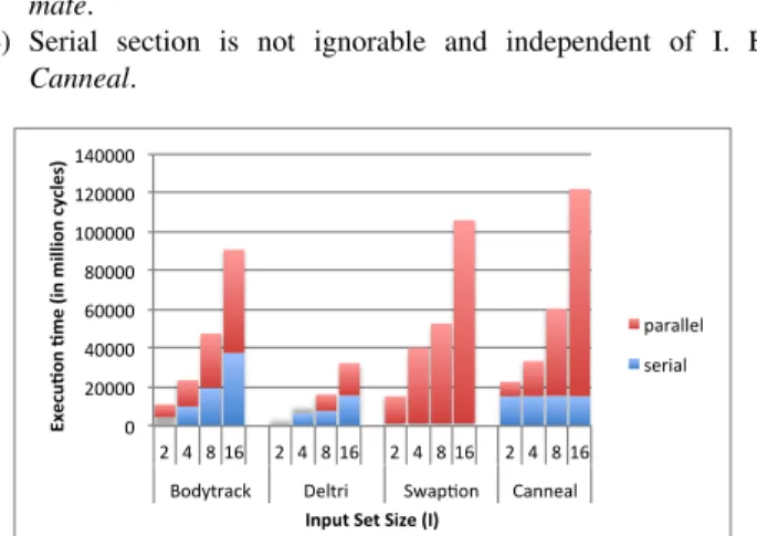
execution time of the serial-section1 increases significantly with the increase in input size, but also at times slightly with the increase in number of processors. Fig. 1 shows four different serial scaling behaviour on different applications when the input set size (I) is increased.
1) Both serial and parallel execution time grows at different rate with I. Eg. Bodytrack.
2) Both serial and parallel execution time grows linearly with I. Eg. Deltri.
3) Serial section is ignorable and independent of I. Eg. Fluidani-mate.
4) Serial section is not ignorable and independent of I. Eg.
Canneal. 0 20000 40000 60000 80000 100000 120000 140000 2 4 8 16 2 4 8 16 2 4 8 16 2 4 8 16 Bodytrack Deltri Swap8on Canneal
Ex e cu& on & m e (in m illion c yc le s) Input Set Size (I) parallel serial
Fig. 1: Different application scaling behaviour with variation in input set size captured in Xeon-phi architecture.
The reason for different serial scaling behaviour among applica-tions can be attributed to the parallelization technique. Multi-threaded programs generally have 3 major phases. 1) the initialization phase where input data are generated, 2) the Region Of Interest (ROI) where the main computation is executed and 3) the finalization phase where the results are processed and the program is terminated. Initialization, finalization phase belong to the serial part and the ROI can belong to both serial and parallel parts depending on the parallelization technique used. In data parallel application, once the threads are spawned they work until the assigned job is complete without any intervention. Here, ROI is totally parallel. This behaviour is observed in swaptions, canneal. On the other hand, the applications that uses pipeline parallelism or a worker thread pool based implementation has a ROI which contributes to the serial part. Here, the master thread does some work to feed the worker threads in ROI and can be a significant contribution to serial section and scales with Input set size. This behaviour is observed in bodytrack, deltri.
Therefore, we build on the observation that not all applications are scaling the same way with the number of processors and the input set size.
Next section describes the empirical model we have built to study application scalability in many-core era.
1We consider serial part of execution is comprised of the sections where
a single thread runs and parallel part consists of the sections where several threads run concurrently.
III. SERIALSCALINGMODEL
Our model’s main objective is to extrapolate the multicore execu-tion behavior of a parallel program to the future many-cores to study their scaling behavior. To keep the model simple, we consider the following:
#1. The execution time is dependent only on input set size I and the number of processors/cores P i,e t(I, P )
#2. An uniform parallel section and an uniform serial section, i.e, we model the total execution time as the sum of serial and parallel execution times as shown in Eq. 3. Both execution times tseq(I, P )
and tpar(I, P ) are complex functions,
t(I, P ) = tseq(I, P ) + tpar(I, P ) (3)
#3. For both the execution times, the scaling with the input set size (I) and the scaling with the number of processors (P ) are independent i,e. tseqand tparcan be modeled as: tpar(I, P ) = Fpar(I)∗Gpar(P )
and tseq(I, P ) = Fseq(I) ∗Gseq(P ). General observation is that, the
execution time of an application with constant input set size reduces with number of threads and the execution time increases gradually when input set size is increased with fixed number of threads. Linear equations do not satisfy the trend and hence, we are using a non-linear power model such that F and G can be represented by a function of
the form h(x) = xα
. Thus, the general form of execution time of the parallel execution is:
t(I, P ) = cseqIasPbs+ cparIapPbp (4)
The SSM model only uses 6 parameters which are obtained empirically to represent the execution time of a parallel application, taking into account its input set and the number of processors. cseq,
as and bs are used to model the serial execution time and cpar, ap and
bp are used to model the parallel execution time. cseq and cpar are
serial and parallel section constants which gives the initial magnitude of the execution time. as and ap are the Input Serial Scaling (ISS) parameter and the Input Parallel Scaling (IPS) parameter. bs and bp are the Processor Serial Scaling (PSS) parameter and the Processor
Parallel Scaling(PPS) parameter.
In the remainder of the paper, we will refer to as, ap, bs and bp as ISS, IPS, PSS and PPS respectively.
In particular, Amdahl’s law and Gustafson’s law can be viewed as two particular cases of the SSM model.
a) A comparison with Amdahl’s Law: Amdahl’s law assumes
a constant input Ibase and an execution time of the serial part
independent from the processor number, i.e. P SS = 0. It also
assumes linear speedup with the number of processors on the parallel part, i.e P P S= −1. Substituting the values in Eq. 4, we get Eq. 5 which shows that execution time is dependent only on P.
t(I, P ) = cseqIbase+
cparIbase
P (5)
b) A comparison with Gustafson’s Law: Gustafson’s law
as-sumes constant execution time for the serial part, i.e. independent of
the working set (ISS= 0) and the number of processors (P SS = 0).
Therefore, tser(I, P ) = cseq. It also assumes that the input is
scaled such that 1) the parallel workload IGus executed with P
processors is equal to P times the “parallel” workload executed in one processor, i.e., IGusap = P . 2) speedup on the parallel part is
linear, i.e. P P S = −1. Substituting the values in Eq. 4, we get
Eq. 6 which shows that time taken to execute remains constant.
In the next section we explain the methodology we adopted to empirically determine the 6 parameters of SSM.
IV. METHODOLOGY
The SSM that we have defined in Eq. 4, should be used to extrapolate performance of (future) parallel applications on large many cores. However, one needs to use realistic parameters. We used the following 3 step methodology on the applications (described in Sec. V) to obtain the 6 SNAS parameters.
Step 1 - Data collection: The application is monitored and Per-formance Monitoring Unit ( PMU) samples (number of instructions executed , number of unhalted clock cycles ) are collected using tiptop [8] at a regular interval of 1ms. Tiptop is a command-line tool for the Linux environment which is very similar to top shell command. Tiptop works on unmodified benchmarks and does not require code instrumentation. The events are counted on per thread basis.
Step 2 - Post processing: The thread wise activity of the applica-tion is analyzed and the execuapplica-tion time spent in the serial and parallel parts are calculated from the number of unhalted clock cycle event. Step 3 - Modeling: The above 2 steps are performed for every application on a given hardware by varying the number of threads(P), the input set size(I) and execution time tseq(I, P ) and tpar(I, P ) are
obtained. Then, we perform a regression analysis with the least-square method to determine the best suitable parameters for the available experimental data.
We used two hardware systems in our experiments, an Intel Xeon E5645 (out of Order) system and an Intel Xeon-Phi 5110P (In-Order) system. These two systems can execute up to 24 and 240 threads respectively. The input set sizes they are able to run are limited by their memory system. Experiments were run on a set of benchmarks we were able to adapt for these architectures.
In the next section, we present the benchmarks used in our experiments.
V. BENCHMARKS
In this study, we focus on applications that will be executed on future manycores. Therefore, we consider benchmarks which are parallelized with shared memory model using Pthreads library. The two conditions that were necessary for our experiments are: 1) Program should be able to run from 2 to 24 (resp. 240) threads. 2) Input sets had to be generated with known scaling factors. We investigated two different categories of benchmark suites as our case study. They are 1. Regular parallel programs from the PARSEC benchmark suite [9] and 2. Irregular parallel programs from the LONESTAR benchmark suite [10].
We studied Bodytrack (body), Canneal (can) , Fluidanimate (fluid)
and Swaptions(swap)in PARSEC. Most of the PARSEC benchmarks
are data parallelized or pipeline data parallelized except for bodytrack which implements a worker-thread pool and has a scalable serial section.
In LONESTAR benchmark suite, we studied Delaunay triangula-tion (deltri), preflowpush (preflow), Boruvka’s Algorithm (Bourvka),
barneshut (barnes), Surveypropogation (survey).
A. Input set scaling
PARSEC benchmark input sets have linear component scaling parameter [11] which are used to scale the input set. Similarly, for LONESTAR we can generate the mesh and graphs with linearly increasing nodes. For some benchmarks like fluidanimate, canneal, swaptions, boruvka and survey we have chosen same input set size on both platforms. But, for other benchmarks we have considered bit
smaller base input set size for xeon-phi compared to xeon because of memory limitations on the platform.
In next section, we validate our model on two diverse architecture platforms:- xeon and xeon-phi.
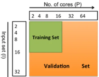
VI. VALIDATION
To validate the model, we use holdout cross-validation method [12] to find the prediction error as shown in Eq. 7 . We divide our obtained data into trainingset and validationset as shown in Figure.2. Training set is a data subset (I≤ 16, P ≤ 16) which is used to tune the model to obtain its parameter values with non-linear regression and validation set is the data subset on which the models prediction capability on the given architecture will be validated. As our model is based on t(I, P ), our data set contains execution time (in million cycles) for the application with given I and P.
Fig. 2: Holdout cross validation showing Training set and Validation set
On Xeon architecture, we validate our model with the validation
set{I=32,P ≤ 24}. The prediction error lies in the range +/- 13%.
We validate our model with the validation set {I=32,P ≤ 128} in
xeon-phi architecture and the prediction error lies in the range +/-30% .
%error = M easuredV alue− P redictedV alue
M easuredV alue ∗ 100 (7)
To show the goodness of fit statistically, we found the absoulte correlation (R-Squared) between observed and predicted values as shown in Eq. 8, where, yiis the observed value,yˆi is the predicted
value of the ith sample in the test set and y is the mean of the¯ samples in test set. In both the architectures R2 was very high in the
range0.9945 ≤ R2 ≤ 0.9999. This means that the predicted value
is almost equal to observed value and data points would fall on the fitted regression line.
R2(y, ˆy) = 1 − P i(yi− ˆyi)2 P i(yi− ¯y)2 (8) VII. INFERENCE
In this section, we explain the inference of the observation using our model and also show how the serial section impacts the speedups of the application with varying I and P.
A. The f parameter
The SSM allows to overcome a major difficulty with previosuly used performance models: the quantification of the parameter f which is usually assumed. With our model, we can find f empirically using Eq. 9. Fraction of parallel part (f) in a program varies with I according to our model. In Eq. 9, we can see that f is basically a function of I (Ibase is a constant base input set size ).
f= tpar(Ibase,1)
tser(Ibase,1)+ tpar(Ibase,1)
= cparI
ap base
cseqIbaseas + cparIbaseap
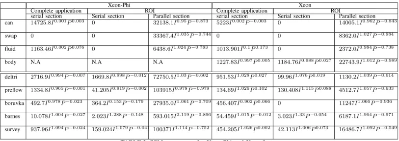
(9) Variation in f for different application are captured in Table. II by varying Input set size (I) from 1 to 10000 on both experimental architectures. We can infer the following:
Xeon-Phi Xeon
Complete application ROI Complete application ROI
serial section Serial section Parallel section serial section Serial section Parallel section
can 14725.8I0.001P0.003 0 32138.1I0.95P−0.873 5223I0.002P−0.003 0 14005.1I0.962P−0.843
swap 0 0 33367.4I1.035P−0.744 0 0 8362.0I1.027P−0.984
fluid 1163.46I0.002P0.076 0 6438.6I1.024P−0.783 1013.901I0.1P0.173 0 2372.0I0.984P−0.738
body N.A N.A N.A 1227.83I0.997P0.005 1184.76I0.988P0.027 22743.9I1.012P−0.989
deltri 2716.9I0.994P−0.007 1669.8I0.998P−0.012 72750.5I1.03P−0.602 951.53I1.028P0.027 99.96I1.076P0.019 1130.2I1.039P−0.614
preflow 1334.8I0.965P−0.001 41.205I0.919P−0.002 103915I0.978P−0.979 134.69I1.026P0.102 130.408I1.115P0.088 4512.7I1.057P−0.633
boruvka 492.7I0.978P−0.023 364.2I0.153P−0.179 27935.0I1.061P−0.709 456.407I0.902P0.066 0 11247I1.066P−0.936
barnes 10.078I1.004P−0.027 2.023I1.288P−0.148 593.015I2.119P−0.896 54.459I1.015P−0.012 3.023I1.33P−0.054 6187.1I1.964P−0.971
survey 937.96I1.094P−0.024 159.024I1.079P−0.041 100371I1.114P−0.752 454.205I1.026P0.002 42.113I1.006P0.073 16486.7I1.092P−0.549
TABLE I: SSM parameters for Xeon-Phi and Xeona
a(N.A means the program was not build-able for the architecture, 0 denotes negligible serial section.)
Xeon Xeon-phi Benchmark 1 10 100 1000 10000 1 10 100 1000 10000 can 0.7284 0.961 0.9956 0.9995 0.9999 0.6858 0.9512 0.9943 0.9994 0.9999 swap 1.0 1.0 1.0 1.0 1.0 1.0 1.0 1.0 1.0 1.0 fluid 0.7006 0.9659 0.9971 0.9998 1.0 0.847 0.9832 0.9984 0.9998 1.0 body 0.9505 0.9531 0.9555 0.9579 0.9601 NA NA NA NA NA deltri 0.5429 0.5494 0.5559 0.5623 0.5687 0.964 0.9668 0.9693 0.9717 0.9739 preflow 0.971 0.9729 0.9747 0.9764 0.9779 0.9873 0.9877 0.9881 0.9884 0.9888 boruvka 0.961 0.973 0.9814 0.9872 0.9912 0.9827 0.9856 0.9881 0.9901 0.9918 barneshut 0.9913 0.999 0.9999 1.0 1.0 0.9833 0.9987 0.9999 1.0 1.0 survey 0.9732 0.9769 0.9801 0.9829 0.9853 0.9907 0.9912 0.9916 0.9919 0.9923
TABLE II: Parallel fraction f for varying Input set size from I=1 to 10000 for xeon and xeon-phi complete applications. #1. Larger the input set size, larger the parallel fraction f in the
program. For example, the f in canneal, fluidanimate in both xeon
and xeon-phi improve with I. In these benchmarks, the serial part is independent of I or constant as we can notice from Table I. In such applications, the larger parallel scaling amortize the lesser scaling serial section.
#2. The impact of the serial scaling can be noticed in deltri, preflow,
bodytrack. In these applications the serial part grows equal to the
parallel part when we increase the input set size. Therefore, the parallel fraction remains almost the same though we increase input set size.
#3. Parallel fraction (f) is not just application dependent but it also depends on the architecture in which it is executed. For example,
we used same Ibase for survey in both the xeon and xeon-phi
architectures but still the f values are different as we increase the input set size. Calculated f values shows that, the parallel fraction of an application is not constant as assumed by Amdahl’s law but varies with the Input set size.
B. Sub-linear scaling
SSM takes into account that the potential speed-up on the parallel section is sub-linear i.e., P P S >−1 in most of the benchmarks. Few benchmarks like swaptions, barneshut and bodytrack in xeon have a
good parallel scaling with −1 ≤ P P S ≤ −0.9 which means that
their speedup can be still in between 1024 to 512 for a processor with 1024 cores. Large number of benchmarks have sublinear scaling in
the range−0.9 ≤ P P S ≤ −0.6 , e.g. canneal, fluidanimate, survey,
deltri, sssp and bfswhere the maximum achievable steedup will be
between 512 and 64 in a 1024 core machine. Added to the sub-linear parallel scaling, SSM also captures the serial scaling effect with ISS and IP S.
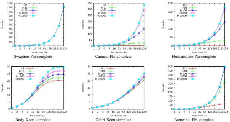
Figure 3 illustrates the potential speedups extrapolated for a few benchmarks varying the processor number from 1 to 1,024 and varying the problem size from 1 to 10,000. The illustrated examples are representative of the behaviours that were encountered among both the chosen architectures. We discuss some of the interesting cases which gives better inference of the SSM parameters and the sub-linear scaling behaviour of the applications.
#1. Some applications are highly scalable. In swaptions, the serial section is so small that it can be ignored in both ROI and complete ap-plication and the parallel section has almost linear scaling in xeon i,e
P P S= −0.984, which shows that such an application may achieve
nearly perfect scaling. On the other hand, the same application
scales sublinearly when executed in xeon-phi with P P S= −0.744.
This behavior can be attributed to the architecural impact on the application.
#2. Some applications have almost constant serial part and rapidly growing parallel part for every input set size. But, large input set sizes are needed to amortize the constant serial part which can be deduced directly from the parameters of the applications. In canneal
complete and fluidanimate complete, large cs
cp, small ISS and P SS
0 100 200 300 400 500 600 700 800 900 1000 1 2 4 8 16 32 64 128 256 512 1024 Speedup No of cores (P) I=1 I=10 I=100 I=1000 I=10000 0 50 100 150 200 250 300 350 1 2 4 8 16 32 64 128 256 512 1024 Speedup No of cores (P) I=1 I=10 I=100 I=1000 I=10000 0 50 100 150 200 250 1 2 4 8 16 32 64 128 256 512 1024 Speedup No of cores (P) I=1 I=10 I=100 I=1000 I=10000
Swaption-Phi-complete Canneal-Phi-complete Fluidanimate-Phi-complete
0 5 10 15 20 25 30 1 2 4 8 16 32 64 128 256 512 1024 Speedup No of cores (P) I=1 I=10 I=100 I=1000 I=10000 0 5 10 15 20 25 30 1 2 4 8 16 32 64 128 256 512 1024 Speedup No of cores (P) I=1 I=10 I=100 I=1000 I=10000 0 50 100 150 200 250 300 350 400 450 500 1 2 4 8 16 32 64 128 256 512 1024 Speedup No of cores (P) I=1 I=10 I=100 I=1000 I=10000
Body-Xeon-complete Deltri-Xeon-complete Barneshut-Phi-complete
Fig. 3: Potential speedups extrapolated for selected benchmarks for varying processor number from P=1 to 1,024 and Input set size from I=1 to 10,000.
scales quasi linearly with I and P. Hence, we can achieve significant improvement in speedup using larger I.
#3. In certain applications, serial part scales on par or at a bit lower
scale compared to the parallel part i,e ISS ≈ IP S and P SS
is sublinear. We can notice such pattern in deltri, preflow, survey,
boruvka, bodytrack completeapplication. These kind of applications
seldom benefit from a manycore system. In these applications we can notice the speedup getting saturated with P despite increasing I due to the serial scaling impact.
#4. Even when the execution time of the serial section is increasing with the input set, it does not always affect the scalability of the application. For instance, in barneshut complete, the execution of the serial section is also increasing with the input set size (ISS= 1.004 ) but at a much lower rate than the execution time of the parallel
section (IP S = 2.1). In such case, if one increases the number of
processors to maintain the execution time constant then the fraction of serial computation time will increase with number of processors and the parallel efficiency will decrease.
C. Heterogeneous architecture
Using many small cores provide more thread level parallelism, but the impact of the serial scaling limits the achievable performance as the time taken to execute the serial section depends on the strength of the core. Hill and Marty [5] show that heterogeneous multicores can offer potential speedups that are much greater than homogeneous multicore chips(and never worse). Heterogeneous cores that feature few very powerful cores, allow the use of an aggressive big core to speedup the serial section to amortize/reduce the impact of serial scaling on the overall performance. By looking at the relative benefits of the larger serial core (relative core strength) i,e tser little
tser big , it is
possible to infer if the application has a potential to benefit from the use of a hybrid core. If the fraction is significantly greater than 1,
then the serial part of the application executes faster in bigger core and we can expect some potential improvement using the hybrid.
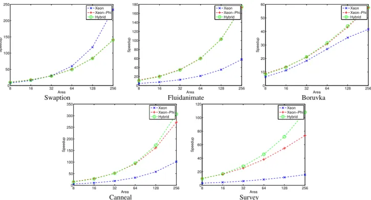
In this paper, we consider a heterogeneous core consisting of one big xeon like core and many small xeon-phi like cores. As Xeon Phi’s area details are still unavailable, we do a pessimistic area-performance analysis with the details of Out-of-Order Xeon (Big core) and In-Order Knights Ferry (Little core) as stated in [13]. Die area per core comparison is around 1:3 between xeon and Knights Ferry i,e 3 little cores can be built in the area of 1 big core. We show 3 different area-performance plots in Fig. 4 where x-axis is the area of Xeon, Xeon-phi and Hybrid equivalent of xeon area and their respective performance in y-axis. The plots are 1. Xeon (all big xeon cores), 2. Xeon-Phi (all Knights Ferry small cores), 3. Hybrid (One big Xeon core which executes serial section and rest Knights Ferry small cores). We will focus only on those benchmarks for which the experiments were carried out with the same input set size in both the platforms as mentioned in Sec.V.
From Table. I, we can see swaption does not have any serial section and hence will not benefit from hybrid architecture. On contrary big xeon cores has good speedup due to their well scaling parallel section. Fluidanimate has a very low core strength and will not have resonable gains from hybrid core. Here, the little and hybrid cores perform better as the application scales better in xeon-phi.
Boruvka has a slightly different behavior. The hybrid will not benefit much here because of the very low core strength. But, interesting observation here is xeon performs on par with xeon-phi because the parallel part scales better in xeon than in xeon-phi.
In canneal, the serial section is fixed and Xeon core is 3X faster than the Xeon-Phi. Therefore, by using a hybrid core we can get better speedup. Moreover, a good parallel section scaling (P P S= −0.873) with many little cores has better performance. Survey also gains better performance using a hybrid core as the big core executes the serial
8 16 32 64 128 256 0 50 100 150 200 250 Area Speedup Xeon Xeon−Phi Hybrid 8 16 32 64 128 256 0 20 40 60 80 100 120 140 160 180 Area Speedup Xeon Xeon−Phi Hybrid 8 16 32 64 128 256 0 10 20 30 40 50 60 Area Speedup Xeon Xeon−Phi Hybrid
Swaption Fluidanimate Boruvka
8 16 32 64 128 256 0 50 100 150 200 250 300 350 Area Speedup Xeon Xeon−Phi Hybrid 8 16 32 64 128 256 0 20 40 60 80 100 120 Area Speedup Xeon Xeon−Phi Hybrid Canneal Survey
Fig. 4: Area-Performance graph showing Hybrid architecture has better speedup with serial scaling. section2X faster than the little core. But, the performance of Xeon
is poor due to the poor parallel section scaling.
VIII. CONCLUSION
Future many-core designs will demand programs with very high degree of parallelism. The available parallelism might be restricted due to the programing techniques used in the application i,e applica-tion inherent behavior or due to the weak underlying hardware which cannot exploit the inherent parallelism in the application.
Currently used traditional models for extrapolating parallel applica-tion performance on multiprocessor- Amdahl’s and Gustafson’s laws - are optimistic as they are very general models. In this work, we have used our own validated model to find out the application scalability of individual applications in a given hardware system. As a result, we can compute the parallel fraction f in a program which is dependent on Input set size I.
Our analysis shows that serial section are not negligible and they may grow with the input set size. Additionally, performance on parallel part does not generally scale perfectly linear with the number of processors that in turn contributes to the limited speedup. Also, from the architectural point of view we have shown how a heterogeneous design with one big core and many small core will help those applications for which the serial section grows with input set size in the many-core era.
ACKNOWLEDGMENT
This work was supported by the European Research Council (ERC) Advanced Grant DAL No 267175. The authors would like to thank Erven Rohou from INRIA Rennes for his insightful help through providing Tiptop for this study.
REFERENCES
[1] J. Parkhurst, J. Darringer, and B. Grundmann, “From single core to multi-core: preparing for a new exponential,” in Proceedings of the 2006 IEEE/ACM international conference on Computer-aided design, ser. ICCAD ’06. New York, NY, USA: ACM, 2006, pp. 67–72.
[2] G. M. Amdahl, “Validity of the single processor approach to achieving large scale computing capabilities,” in Proceedings of the April 18-20, 1967, spring joint computer conference, ser. AFIPS ’67 (Spring). New York, NY, USA: ACM, 1967, pp. 483–485.
[3] J. L. Gustafson, “Reevaluating amdahl’s law,” Commun. ACM, vol. 31, no. 5, pp. 532–533, May 1988.
[4] B. Juurlink and C. H. Meenderinck, “Amdahl’s law for predicting the future of multicores considered harmful,” SIGARCH Comput. Archit. News, vol. 40, no. 2, pp. 1–9, May 2012.
[5] M. D. Hill and M. R. Marty, “Amdahl’s law in the multicore era,” Computer, vol. 41, no. 7, pp. 33–38, 2008.
[6] S. Eyerman and L. Eeckhout, “Modeling critical sections in amdahl’s law and its implications for multicore design,” in Conference Proceedings Annual International Symposium on Computer Architecture. Associa-tion for Computing Machinery (ACM), 2010, pp. 362–370.
[7] L. Yavits, A. Morad, and R. Ginosar, “The effect of communication and synchronization on amdahl¯ał s law in multicore systems,” Parallel Computing, vol. 40, no. 1, pp. 1–16, 2014.
[8] E. Rohou, “Tiptop: Hardware Performance Counters for the Masses,” INRIA, Rapport de recherche RR-7789, Nov. 2011.
[9] C. Bienia, S. Kumar, J. P. Singh, and K. Li, “The parsec benchmark suite: Characterization and architectural implications,” in Proceedings of the 17th international conference on Parallel architectures and compilation techniques. ACM, 2008, pp. 72–81.
[10] M. Kulkarni, M. Burtscher, C. Casc¸aval, and K. Pingali, “Lonestar: A suite of parallel irregular programs,” in Performance Analysis of Systems and Software, 2009. ISPASS 2009. IEEE International Symposium on. IEEE, 2009, pp. 65–76.
[11] C. Bienia and K. Li, “Fidelity and scaling of the parsec benchmark inputs,” in Workload Characterization (IISWC), 2010 IEEE International Symposium on, 2010, pp. 1–10.
[12] L. Liu and M. T. ¨Ozsu, Eds., Encyclopedia of Database Systems. Springer US, 2009.
[13] T. Hruby, H. Bos, and A. S. Tanenbaum, “When slower is faster: On heterogeneous multicores for reliable systems,” in Proceedings of USENIX ATC, USENIX. San Jose, CA, USA: USENIX, June 2013.