IRISA at DeFT 2015: Supervised and Unsupervised Methods in Sentiment Analysis

(1)

HAL Id: hal-01226528

https://hal.archives-ouvertes.fr/hal-01226528v2

Submitted on 17 Mar 2016

HAL is a multi-disciplinary open access

archive for the deposit and dissemination of

sci-entific research documents, whether they are

pub-lished or not. The documents may come from

teaching and research institutions in France or

abroad, or from public or private research centers.

L’archive ouverte pluridisciplinaire HAL, est

destinée au dépôt et à la diffusion de documents

scientifiques de niveau recherche, publiés ou non,

émanant des établissements d’enseignement et de

recherche français ou étrangers, des laboratoires

publics ou privés.

Methods in Sentiment Analysis

Vedran Vukotić, Vincent Claveau, Christian Raymond

To cite this version:

Vedran Vukotić, Vincent Claveau, Christian Raymond. IRISA at DeFT 2015: Supervised and

Unsu-pervised Methods in Sentiment Analysis. DeFT, Défi Fouille de Texte, joint à la conférence TALN

2015, Jun 2015, Caen, France. �hal-01226528v2�

(2)

IRISA at DeFT 2015: Supervised and Unsupervised Methods in Sentiment

Analysis

Vedran Vukotic

Vincent Claveau

Christian Raymond

INRIA

1

– CNRS

2

– INSA de Rennes

3

– IRISA

1,2,3

,

Campus de Beaulieu, 35042 Rennes cedex

{vedran.vukotic, vincent.claveau, christian.raymond}@irisa.fr

Résumé.

Cet article décrit la participation de l’équipe LinkMedia de l’IRISA à DeFT 2015. Notre équipe particpé à deux tâches : la classification en valence des tweets (tâche 1) et la classification à grain fin, elle même, décomposée en deux sous-tâches, à savoir la détection des classes génériques de l’information exprimée dans un tweet (tâche 2.1) et la classification des classes spécifiques (tâches 2.2) de l’émotion/sentiment/opinion exprimée. Pour ces trois tâches, nous adoptons une démarche d’apprentissage artificiel. Plus précisément, nous explorons l’intér de trois méthodes : i) le boost-ingd’arbres de décision, ii) l’apprentissage bayésien utilisant une technique issue de la recherche d’information, et iii) les réseaux neuronnaux convolutionnels. Nos approches n’exploitent aucune ressource externe (lexiques, corpus) et sont uniquement fondées sur le contenu textuel des tweets. Cela nous permet d’évaluer l’intérêt de chacune de ces méthodes, mais aussi des représentations qu’elles exploitent, à savoir les sacs-de-mots pour les deux premières et le plongement de mots (word embedding) pour les réseaux neuronaux.

Abstract.

IRISA participation at DeFT 2015: Supervised and Unsupervised Methods in Sentiment Analysis

In this work, we present the participation of IRISA Linkmedia team at DeFT 2015. The team participated in two tasks: i) valence classification of tweets and ii) fine-grained classification of tweets (which includes two sub-tasks: detection of the generic class of the information expressed in a tweet and detection of the specific class of the opinion/sentiment/emo-tion. For all three problems, we adopt a standard machine learning framework. More precisely, three main methods are proposed and their feasibility for the tasks is analyzed: i) decision trees with boosting (bonzaiboost), ii) Naive Bayes with Okapi and iii) Convolutional Neural Networks (CNNs). Our approaches are voluntarily knowledge free and text-based only, we do not exploit external resources (lexicons, corpora) or tweet metadata. It allows us to evaluate the interest of each method and of traditional bag-of-words representations vs. word embeddings.

Mots-clés :

Fouille d’opinion, apprentissage artificiel, boosting, apprentissage bayésien, plongement de mots.

Keywords:

Opinion mining, machine learning, boosting, Bayesian learning, word embedding.

1 Introduction

All the three classification problems analyzed in this paper are sentiment analysis problems. They consist of the same data samples, French tweets, whose target labels vary according to the task. After describing these classification tasks and their corresponding datasets in Section 1, we present and analyze the classifiers used in this work. In section 2, decision trees with boosting are applied directly to symbolic words. Section 3 describes a system consisting of Bayesian learning relying on information retrieval techniques. Section 4 deals with Convolutional Neural Networks (CNNs) combined with various word embedding methods. Finally, in section 5, all the three systems are compared for the three classifications tasks and a conclusion is given in section 6.

(3)

1.1 Task 1: valence classification

The provided training set consists of 7929 tweets, 102 of which were not found at the time of retrieval. Each sample belongs to one of the following three classes: positive (+), negative (-) and neutral/mixed (=). The distribution of the classes in the training set is sufficiently uniform: 31% (+), 24% (-) and 45% (=).

1.2 Task 2.1: detection of the generic class of the information

The provided training set for this task consists of 6754 tweets, 81 of which were not found at the time of retrieval. Each sample in this task belongs to one of the following four classes: information, opinion, sentiment and emotion. The classes are not very well distributed within this task, thus possibly introducing biases in the classifiers: 53% (INFORMATION), 34% (OPINION), 1% (SENTIMENT) and 12% (EMOTION).

1.3 Task 2.2: detection of the specific class of the opinion/sentiment/emotion

For this task, 3183 tweets were provided, 40 of which were not found during retrieval. There are 18 classes in this task: negative surprise / negative astonishment (SURPRISE_NEGATIVE), agreement / understanding / approbation (AC-CORD), sadness / sorrow / suffering / despair / resignation (TRISTESSE), valorization / interest / appreciation (VAL-ORISATION), dissatisfaction / unhappiness (INSATISFACTION), fear / terror / worry / anxiety (PEUR), appeasement / relief / gratefulness / forgiving / serenity (APAISEMENT), anger / rage / irritation / exasperation / nervousness / impa-tience (COLERE), satisfaction / contentment / pride (SATISFACTION), disagreement / disapprobation (DESACCORD), displeasure / deception (DEPLAISIR), disturbance / embarrassment (DERANGEMENT), love / sweetness / affection / devotion / passion / envy / desire (AMOUR), contempt / disdain / disgust / hate (MEPRIS), pleasure / entertainment / joy / euphoria / happiness / ecstasy (PLAISIR), positive surprise / positive astonishment (SURPRISE_POSITIVE), boredom (ENNUI), devalorization / disinterest / depreciation (DEVALORISATION).

In this task, the classes are also not well balanced and could thus introduce a bias into the classifiers: 4.8% (AC-CORD), 0.3% (AMOUR), 0.3% (APAISEMENT), 6.6% (COLERE), 1.5% (DEPLAISIR), 0.4% (DERANGEMENT), 6.8% (DESACCORD), 12.6% (DEVALORISATION), 0.1% (ENNUI), 0.3% (INSATISFACTION), 5.5% (MEPRIS), 8.6% (PEUR), 1.1% (PLAISIR), 2.3% (SATISFACTION), 0.3% (SURPRISE_NEGATIVE), 0.1% (SURPRISE_POSITIVE), 1.1% (TRISTESSE), 47.3% (VALORISATION). Also, it is worth noticing that this task has the least samples and the most classes, which together with their nonuniform distribution is negatively effecting the learning of meaningful decision boundaries.

1.4 Test set

The test set of the DeFT 2015 challenge consists of 3383 tweets (2 of which were not found at the time of retrieval for some participants and were removed by the DeFT commission). The correct target labels were unknown at the time of developing the methods described in this articles, so all the experiments performed and described are done on splits of the provided training data into train, validation and test sets, as described in each of the following sections. The performance of our methods on the official test set is given at the end of this article.

2 Boosting decision trees

In order to tackle the three tasks presented in the introduction, we first adopt a standard Machine learning approach based: boosting decision Trees. This approach, using a very usual text representation of the tweets, is intended to be a baseline. In this section, we first describe the principles of this machine learning technique and then the performance obtained with the training dataset.

(4)

Task Parameters Macro-precision Micro-precision

Task 1 n = 2000d = 4 0.702 0.684

Task 2.1 n = 100d = 3 0.712 0.717

Task 2.2 n = 100d = 10 0.427 0.625

Table 1: Performance of Bonzaiboost in a 10-fold cross-validation

2.1 Principles

Decision Trees are well-known classifiers based on a succession of test on the features of an example in order to determine its class. They can be easily inferred from training examples, they can deal with numeric or symbolic features, and they are able to handle any number of classes.

In our case, in order to achieve better performance, several Decision Trees are inferred and from the training data and combined following the popular boosting algorithm AdaBoost.MH (Schapire & Singer, 2000). This meta-learning frame-work is an iterative process, in which errors (tweets receiving the wrong class label) obtained with the tree inferred at the previous step are given more weight so that the next decision tree will focus more on this problematic examples.

The implementation that we used in our experiments is BONZAIBOOST1.

2.2 Practical details and performance

The tweet are represented as sets of words (unigrams) in order to be manipulated by the decision trees. The test used in the nodes of the trees is thus just to check if a tweet contains a word or not.

Boosting was first proposed to improve the classification performance of weak learners, that is, classifiers with a low precision (though it has also be shown to improve results of strong classifiers). Thus, in the case of Decision Trees, boosting is often used with low depth trees (Antoine Laurent & Raymond, 2014), such as decision stumps (depth=1). During the training phase, we experimented with several number of iterations (n) for boosting and several depth of trees (d). These two parameters (n and d) were chosen through cross-validation in order to maximize the macro-precision, as it is the main score proposed by the organizers. The best performance is found for d = and n =; they are summarized in Table 1. Yet, it is noteworthy that several other settings (n and d) gave very close results. This is due to the fact that macro-precision is a very unstable score, since a simple tweet, if it is correctly or incorrectly classified in a class with very few tweets, can drastically change the final score.

One interesting thing with decision trees is that they can be interpreted, to some extents. It is even easier with decision stumps since one can directly see the (only) test, that is, in our case, the presence or absence of a word in a tweet, with the label of the class and a weight. Moreover, when using boosting over decision stumps, we get a high number of decision stumps, and thus a high number of these word/label/weight associations. They may be gathered to form a lexicon suited to the set of class used in the tasks. For instance, here is a small excerpt of such a lexicon concerning the word menace for Task 2.2 in which one can see that menace is strongly associated with PEUR, and to the contrary, strongly opposed to VALORISATION.

(5)

word label vote menace ACCORD -1.450 menace AMOUR -0.626 menace APAISEMENT -0.473 menace COLERE -1.447 menace DEPLAISIR -1.100 menace DERANGEMENT -0.411 menace DESACCORD -1.520 menace DEVALORISATION 0.219 menace ENNUI -0.306 menace INSATISFACTION -0.797 menace MEPRIS -1.321 menace PEUR 2.132 menace PLAISIR -1.046 menace SATISFACTION -1.023 menace SURPRISE_NEGATIVE -0.741 menace SURPRISE_POSITIVE -0.266 menace TRISTESSE -1.042 menace VALORISATION -2.195

3 Bayesian learning

In this section we present the second machine learning approach tested by IRISA for Tasks 1, 2.1 and 2.2. As for the previous one, it relies on a simple representations of text, that is bags-of-words. It is a somewhat classical framework based on Bayesian learning whose only originality is to use Information Retrieval techniques in order to estimate certain probabilities needed to predict class labels of the tweets.

3.1 Principles

Let us note ωi the label of one the class and dj is the description of one of the tweets. Under a probabilistic framework, the goal of the task can be expressed as finding the class that maximizes this probability P (ωi|dj), i.e.

ω∗= arg max i

P (ωi|dj)

By using the well-known Bayesian rule, this probability can be decomposed into: P (ωi|dj) =

P (dj|ωi) ∗ P (ωi) P (dj) Moreover, since P (dj) is constant for a given tweet, we have:

ω∗= arg max i

P (dj|ωi) ∗ P (ωi)

Finally the two probabilities to estimate on the training data are the a priori probability of a class P (ωi) and the likelihood P (dj|ωi).

In this work, the a priori probability is simply estimated by counting the number of tweets of each class, and by smoothing (Laplace smoothing) not to put a disadvantage on less populated classes:

P (ωi) =

nb tweets of class omegai+ 1 nb tweets + nb classes

The main originality of our approach is to use an information retrieval technique in order to estimate the likelihood of a tweet given a class. For a given tweet, we use a k-nearest-neighbors approach: the k closest training tweets are retrieved by using an information retrieval system. More precisely, we use a system based on Okapi-BM25 (Robertson et al., 1998)

(6)

Task Macro-precision Micro-precision Task 1 0.679672521722188 0.615226864906434 Task 2.1 0.792678272906324 0.641901037750038 Task 2.2 0.449395650820018 0.590676883780332

Table 2: Performance of Bayesian learning on the training set (10-fold cross validation)

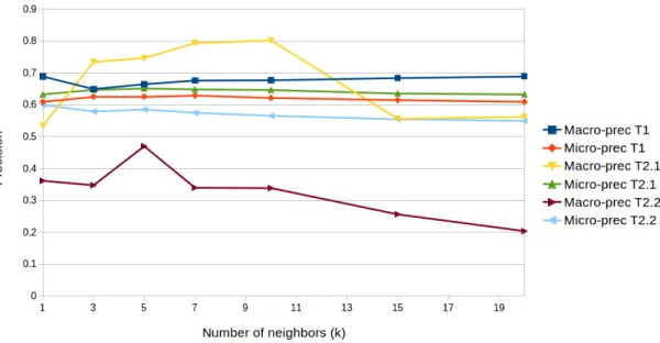
Figure 1: Macro and micro-precisions for Tasks 1, 2.1, 2.2 according to k

which has proven robust and efficient in many information retrieval or extraction tasks. The considered tweet is thus considered as a query q, containing words noted ti. A score is computed for each training tweet d, as follows (df gives the document frequency of a word, dl gives the document length, dlavgis the average document length in the collection, k1= 1, b = 0.75 and k3= 1000 are constants):

scoreBM 25(d) = X ti qT F (ti, q) ∗ T FBM 25(ti, d) ∗ IDFBM 25(ti) = X ti (k3+ 1) ∗ tf (ti, q) k3+ tf (ti, q) ∗ tf (ti, d) ∗ (k1+ 1) tf (ti, d) + k1∗ (1 − b + b ∗ dl(d)/dlavg) ∗ logN − df (ti) + 0.5 df (ti) + 0.5 (1)

From the k tweets with highest scores, we estimate the likelihood of the tweet for a given class as the proportion of tweets from this class in these k neighboring tweets.

3.2 Practical details and performance

For our experiments, the value for k was tuned on the training set through leave-one-out in order to maximize the macro-precision. The values found are k = 10 for task 1, k = 10 for task 2.1 and k = 3 for task 2.2.

The performance of our Bayesian learning approach is shown in table 2. It is computed with a 10-fold cross-validation over the training dataset.

In order to illustrate the influence of the number of neighbors considered when computing the likelihood, Figure 1 presents the macro and micro-precisions for each task, according to different values of k. One can notice that this value has only a limited influence on micro-precision (about 0.05 between maximum and minimum micro-precision values. Concerning macro-precisions, the situation is contrasted: for Task 1, k has a small influence. It is easily explained by the fact that there many tweets for each class, and thus it does not influe on the kNN process. Conversely, for Task 2.1 and 2.2, macro-precisions varies a lot. This is due to the fact that for some classes with very few training data, if k gets higher

(7)

than the population of the class, the kNN will necessarily includes tweets from other classes. This fact is made worse by the instability of the macro-precision score (see Section 5.3), since tweets from these less populated classes will tend to be misclassified, even if the number of misclassified tweets do not vary so much globally.

4 Convolutional Neural Networks

Deep learning methods have been shown to produce state-of-the-art results in various tasks and different modalities (vision, speech, etc.). Convolutional Neural Networks (LeCun & Bengio, 1995) represent one of the most used deep learning method in visual recognition. Recent works have shown that CNNs are also well suited for sentence classification problems and can produce state-of-the-art results (Kim, 2014; Johnson & Zhang, 2014). These studies have analyzed the performance of CNNs in datasets like movie reviews, the Stanford sentiment treebank, customer reviews and similar datasets that usually consists of positive/negative labels (either binary or with fine-grained intensities). In this section, we explore the feasibility and measure the performance of similar CNN models in multi-class emotion classification of short sentences (tweets).

CNNs consist of a series of interchanged convolutional and pooling layers, followed by a simple classifier (usually a MLP or an RBF). CNNs have two interesting properties that make them valuable and robust classifiers in computer vision: i) autonomous learning of meaningful features and ii) robustness to spatial variations (translational invariance).

Convolutional layers scan the inputs of the previous layer with learned kernels. The kernels are learned by backpropa-gation and become filters that respond to features relevant for the classification task. By applying multiply convolutional layers, the network learns meaningful features at different levels.

Pooling layers reduce the dimensionalites of their respective previous layers either by different downsampling methods or by more complex pooling methods that use different metrics. The most common pooling method in CNNs i s max-pooling. Max-pooling have been shown to provide good results while also being very computationally inexpensive (Boureau et al., 2010).

A typical approach in machine learning for improving generalization consists of combining different architectures. How-ever, that can be computationally expensive. The dropout method suggest randomly disabling some hidden units during the training part, thus generating a big set of combined of virtual classifiers without the computational overhead (Hinton et al., 2012). For a simple multilayer perceptron with N neurons in one hidden layer, an equivalent of 2N virtual ar-chitectures would be generated by applying dropout. Dropout has been shown to significantly improve generalization of CNNs.

CNNs have recently been shown to be useful and perform well in NLP classification problems (Kim, 2014). The difference between CNNs applied to computer vision and their equivalent in NLP lies in the input dimensionality and format. In computer vision, inputs are usually single-channel (eg. grayscale) or multi-channel (eg. BGR) matrices (2D), usually of constant dimensions. In sentence classification, each input consist of a sequence of words of non-constant length. Each word w is represented with a numerical vector (embedding) ~ewof a constant size. Word embeddings can be learned jointly, with the classifier, in a supervised manner or separately, usually in a unsupervised manner (eg. word2vec (Mikolov et al., 2013)). All the word representations are then concatenated (in their respective order) and padded with zero-vectors to a fixed length (maximum possible length of the sentence). Eg. the phrase "Que la force soit avec toi #4mai" would be represented to the CNN input as ~x = ~eque⊕ ~ela⊕ ~ef orce⊕ ~esoit⊕ ~eavec⊕ ~etoi⊕ ~eT AG⊕ ~eU N KN OW N⊕ ~0 ⊕ . . .~0 with |~xi| = const., ∀i, where the ⊕ operator represents concatenation. Although this representation may look counter-intuitive from a more classical NLP viewpoint, it is a perfectly good representation for a CNN, due to their translational invariance property that enables them to be robust to changes in position within sentences, while still being able to grasp relevant features from the words and their context.

4.1 Model description

The model used in this work shares the same architecture as the simple model in (Kim, 2014): a single convolutional layer, followed by a max-over-time (Collobert et al., 2011) pooling layer and a standard soft-max fully connected layer at the end. A standard dropout of 0.5 (50% of the neurons are disabled in each iteration) is used.

(8)

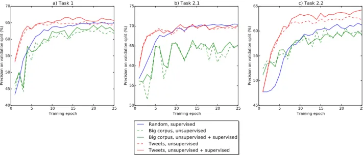
training set of a 5-folds validation) is first randomly split into a smaller training set (90%) and a validation set (10%). Figure 2 shows the errors of the validation sets for different variations that will be described in the following subsections. Prior to converting words to their numerical representation (word embedding), all the sentences were preprocessed in the following manner: all the words were converted to their lowercase equivalent; punctuation marks were isolated into separate elements; URLs and references were converted to respective tags ("<url>" and "<ref>"); finally, hashtags were converted to two separate elements: a tag and the original hashtag string (eg. "#nowplaying" → "<tag> nowplaying").

0 5 10 15 20 25 Training epoch 40 45 50 55 60 65 70

Precision on validation split (%)

a) Task 1 0 5 10 15 20 25 Training epoch 50 55 60 65 70 75

b) Task 2.1

Random, supervised Big corpus, unsupervised

Big corpus, unsupervised + supervised Tweets, unsupervised

Tweets, unsupervised + supervised

0 5 10 15 20 25 Training epoch 45 50 55 60 65

c) Task 2.2

Figure 2: Performance comparison of various text embedding methods with CNNs

4.2 Randomly initialized word embeddings

In these experiments, word embeddings were initialized randomly from a uniform distribution U (−0.25, 0.25). After-wards, the embeddings were trained in a supervised manner together with the CNN. This works by simply by extending backpropagation to the layer before the first convolutional layer (the lookup table). As seen is in figure 2, this method takes a significant number of epochs more to converge to a stable precision, but does perform quite well. It can be noticed that in Task 2.2 (figure 2 c.), due to the biggest number of classes and the least number of examples, it converged slower and with less good precision on the validation sets.

4.3 Word embeddings learned on a big corpus

These six experiments used external big corpuses to train embeddings for the French language in an unsupervised manner. It is important to note that obviously these embeddings had no special knowledge (an appropriate representation) of Twitter specifics (hashtags, references, URLs, etc.). Embeddings of unknown words are initialized randomly and are later either fine-tuned in a supervised manner or not. For each task, two variations were analyzed: one in which the embeddings learned in an unsupervised manner were kept static and one in which they were updated (fine-tuned) while learning the CNNs. The latter has been shown to perform slightly better but with no significant differences.

Compared to random embeddings, these embeddings trained on large corpora have a slight initial advantage but do not perform as well after more training epochs. Our explanation for this phenomena is that in such tasks, having a notion of the twitter specifics within the embeddings is advantageous and the method lacks that advantage.

4.4 Word embeddings learned on DeFT tweets

Here, we describe six experiments with embeddings learned directly from the tweets (the training set of the current fold) in an unsupervised manner, with word2vec (Mikolov et al., 2013): three with static embeddings and three with furtherly

(9)

Emb. initialization Fine-tuning Macro-precision Micro-precision Task 1

Random Supervised (CNN backpropagation) 0.651662928327043 0.653123802223074

Big corpus (unsupervised) Supervised (CNN backpropagation) 0.624707901585991 0.626038073335889

Big corpus (unsupervised) - 0.615873905343281 0.614283889101827

Tweets (unsupervised) Supervised (CNN backpropagation) 0.657463685838549 0.66002299731698

Tweets (unsupervised) - 0.651445850997478 0.652484987862527

Task 2.1

Task 2.2

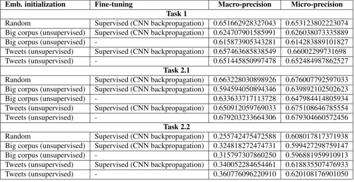
Table 3: Performance analysis of various embedding methods and CNNs in a 5-fold cross-validation

fine-tuned embeddings (in a supervised manner, while performing backpropagation on the CNNs).

These methods seem to perform the best. The unsupervised representation learning brought initial advantage (faster convergence). Fine-tuning the embeddings contributed to a very small advantage, except for task 2.2 where the supervised fine-tuning brought a significant advantage.

Combining embeddings learned in an unsupervised manner directly on the tweets (thus enabling them to have notions of Tweeter specifics) and fine tuning them in a supervised manner while training the CNNs is the best choice for this kind of tasks, especially if there is a significantly small number of training samples and a bigger number of classes, like in task 2.2.

4.5 Performance

Table 3 shows the results of the various methods with CNNs described in this section. Macro and micro precisions are computed with the official DeFT 2015 evaluation tool. Only macro-precision is evaluated during for the challenge, but here, we report also micro-precision as it might provide a better performance measure for this type of multiclass classification problems.

All the methods were evaluated with a 5-folds cross-validation (80% training and 20% test for each fold). It is clear that the best methods consists of training word embeddings in an unsupervised manner directly on tweets. Additionally supervised fine-tuning improves the performance, but just slightly.

Training embeddings in generic big corpus for specific classification tasks (like short tweets) does not seem to be a feasible method.

Random initialization of embeddings and supervised learning seems to also be feasible. One could think that this method is faster than training unsupervised embeddings first, but unsupervised word representation methods like word2vec (Mikolov et al., 2013) are very fast (especially in small datasets like this one) and significantly improves the speed of convergence and precision.

(10)

Method Macro-precision Micro-precision Task 1

Bonzaiboost 0.6723841209 0.5995856762

Bayesian learning 0.6985095279 0.6898490678

CNN, word2vec on tweets + supervised fine tuning 0.6580527369 0.6531518201 Task 2.1

Bonzaiboost 0.4779050332 0.52352767091

CNN, word2vec on tweets + supervised fine tuning 0.5020312287 0.57147084937 Task 2.2

Bonzaiboost 0.2577236629 0.5157972079

CNN, word2vec on tweets + supervised fine tuning 0.3159632639 0.5525349008

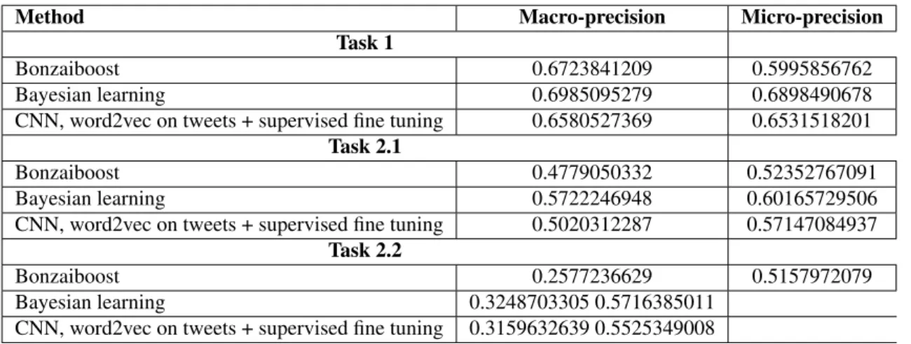
Table 4: Performance of the three proposed methods on the official DeFT 2015 test set

5 Performance comparison and discussion

5.1 Official results

The DeFT 2015 accepted three submissions (runs) per team. We opted to submit one run from Bayesian learning, one with Bonzaiboost and a last one from the CNN method with embeddings learned on tweets and fine tuned. It is important to notice that cross-validations differ in the experiments described in this paper prior to the final official evaluation (eg. CNNs use a 5-fold cross-validation while Naive Bayes was evaluated with a 10-fold cross-validation). The most indicative performance evaluation is thus given on the official DeFT 2015 test set and is shown in table 4.

Bayesian learning performed best in tasks 1 and 2.1. CNNs performed best in Task 2.2. This improvement of CNNs performances in multiclass data with less samples is due to gain brought by the directly learned embeddings. It is important to note that there should be room for improvement in CNNs to close the gap in simpler datasets (task 1 and 2.1) and probably improve upon the other results. We think that it would be valuable to research applying the same embeddings to a deeper CNN (more than one convolutional and one pooling layer) thus enabling the network to grasp concepts at greater distances within a sentence.

The difference observed between these values and the one estimated on the training set (10 points in macro-precision), especially for task 2.2, is left unexplained. A technical problem or the choice of wrong parameters may explain that, as well as a difference when building the training and the test sets. But we also give additional thoughts on the fact that the macro-precision was not a reliable choice in order to chose the best parameters (see below).

5.2 Data inconsistencies and its consequences

The training data contains many tweets whose provided label, whatever the tagset (ie. task 1, 2.1 or 2.2), is hard to explain. For instance, consider the following tweets:

INFORMATION @ONPCofficiel Sortir du nucléaire oui, à condition

d’avoir des nouvelles énergies plus écologiques, Cécile Duflot!

POSITIVE_SURPRISE @LoireBretagne On s’étonne qu’elle soit ouverte, cette

pêche à l’anguille. Sauf si pêcher une espèce menacée

est une forme de protection...

This even more problematic with less-populated classes; here are three of the eight tweets labeled as AMOUR (task 2.2) in the training data.

(11)

AMOUR . @RoyalSegolene "Les Français souhaitent à 90% le développement des énergies renouvelables" http://t.co/TYyr2jFR81

AMOUR j’ai envie d’autres paysages que le vide et les cinq

pauvres éoliennes de l’aube

AMOUR Les sénateurs écologistes fans de @RoyalSegolene »

http://t.co/kSP3l2cv5s

Most striking, very similar tweets may receive different annotations (here, labels for tasks 1 and 2.1):

+/NONE @fanph94 3/4: Lorsque la combustion est optimum, les

particules fines émises sont composées de sels alcalins peu nocifs

=/INFORMATION @fanph94 4/4: Combustion de qualité + combustible

sec et propre = quantités de particules fines émises réduites et moins nocives

This inconsistencies are even more obvious with quasi-identical tweets:

=/INFORMATION #TribunedeGenève . L’Etat s’est trouvé face à un

Diogène industriel: Trois cents tonnes de déchets

toxiques à ... http://t.co/b4lJ9UsBrS

+/NONE L’Etat s’est trouvé face à un Diogène industriel: Trois

cents tonnes de déchets toxiques à assainir. ...

http://t.co/m8MeDGAvRg #Genève

=/INFORMATION Développement durable : 20 ans après le Caire, l’ONU

réaffirme le rôle central des gens: A l’ouver...

http://t.co/q9gD1sMXOQ RT @Mediaterre

+/OPINION Développement durable : 20 ans après le Caire,

l’ONU réaffirme le rôle central des gens http://t.co/XCaVGb16F6

+/OPINION Développement durable : 20 ans après le Caire,

l’ONU réaffirme le rôle central des gens http://t.co/LUelHU4flR #ecologie Mediaterre

Of course, such inconsistencies question the validity of the evaluation since the test set certainly contains identical flaws. They are also harmful for any machine learning technique during the training step. Unfortunately, this is more specifically the case for our Bayesian learning, to some extent, and for boosting. Concerning The former, one can easily understand that the kNN used to compute the likelihood will make its decision based on very close or similar examples. A similar example with a wrong label will chiefly biase the decision, especially when k is small. Thus, these inconsistencies are more particularly harmful for task 2.2, where the small number of examples for certain class requires us to set k to such small values. The boosting is also known to sensible to low quality training data. Since more weight is given to misclassified examples at each iteration, the inconsistent examples presented above will receive more and more weight and thus biased the final combination of weak learners (Philipp M. Long, 2010)

5.3 Discussion about the stability of macro-precision

The choice of macro-precision as the main evaluation score raise several issues. As it was explained before (cf. Sec. 3.2), this choice, combined with the fact that classes are strongly unbalanced (especially for task 2.2), is not well taken into

(12)

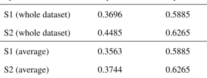
System macro-precision micro-precision

S1 (whole dataset) 0.3696 0.5885

S2 (whole dataset) 0.4485 0.6265

S1 (average) 0.3563 0.5885

S2 (average) 0.3744 0.6265

Table 5: Macro and Micro-precisions computed over the dataset as a whole or divided into 30 subsets

account by our simple machine learning frameworks.

The other problem we want to stress here is the instability of this score. As said earlier the correct or incorrect classification of a single tweet, in a less-populated class, may have a strong impact on the final result. It means that the difference between two systems’ macro-precisions, is not necessarily statistically significant, even if the difference itself may appear as important. In order to illustrate that point, we consider two systems S1 and S2 based on on our boosting approach with sligthly different settings. S1 and S2 uses n = 100 iterations, but S1 builds decision stumps (d = 1) while the maximal depths for S2 is d = 10. These two systems are trained and evaluated on the training dataset (through 10-fold cross-validation) on task 2.2. The micro and macro-precisions for the whole dataset (concatenation of the 10 test folds) are given in Table 5. It is worth noting S2 performs better than S1; the difference between the two systems’ macro-precision is high, and also important in a smaller extent in terms of micro-precisions. In order to study the stability of these scores, we also divide the dataset into 30 equal parts and compute for each of them and for each system the two scores. Thus, we have 30 macro-precisions and 30 micro-precisions for S1 and the same for S2. We indicate the average precisions over these 30 subsets in the Table 5. It appears that the average macro-precision for S2 is in fact much lower than when considering the dataset as a whole. In order confirm that, we compute a paired Student t-test between these two systems with the 30 pairs of scores. The p-value for the macro-precision is p = 0.2582, and the micro-precision’s one is p = 0.00045. It means that the difference of macro-precision between S1 and S2 is not statistically significant, while the micro-precision difference can be considered as statistically significant.

This tends to demonstrate that macro-precision computed over a whole dataset of tweets is not a reliable score to evaluate the systems, especially when some classes only contains a few tweets, as it is the case for several classes of Task 2.2. Another side-effect is that using macro-precision to chose the final parameters of our machine learning techniques has certainly led us to pick up sub-optimal solutions.

6 Conclusion

For this participation of IRISA to Tasks 1, 2.1 and 2.2 of DeFT2015, we focused on Machine learning approaches ex-ploiting only the texts of the tweets, with no external knowledge sources or metadata. Our goal was mainly to examine the interest of embeddings over traditional bag-of-words approach. We showed that traditional methods outperform sim-ple deep methods (CNNs) in tasks with less classes and a sufficient number data samsim-ples for each class. Yet, for more complex tasks, deep learning has been shown to be a competitive approach, especially when combined with embeddings previously learned in an unsupervised manner and fine tuned during classification. Yet, the added-value is not proven and simple bags-of-words still appear as competitive.

The question of whether a deeper CNN architecture would be able match standard methods or even outperform them on all datasets is open for further future experimentation. Another point to investigate is the difference of results between train set (with cross-validation) and the test-set.

From the point of view of the tasks itself, we have pointed some inconsistencies in the ground-truth and explained how they challenged our machine learning techniques. More importantly, we have shown that the macro-precision is a too unstable score to evaluate the systems directly, at least for Task 2.2 in which some classes contains only a few tweets. As a result, the rankings of the participants based on this sole score, is unfortunately not reliable. On the contrary, micro-precision appears much more stable score and is more naturally optimized by usual machine learning frameworks.

(13)

Acknowledgement

This work was partly funded via the CominLabs excellence laboratory financed by the National Research Agency under reference ANR-10-LABX-07-01.

7 Bibliography

ANTOINELAURENTN. C. & RAYMONDC. (2014). Boosting bonsai trees for efficient features combination : applica-tion to speaker role identificaapplica-tion. In Proc. of InterSpeech.

BOUREAUY., PONCEJ. & LECUNY. (2010). A theoretical analysis of feature pooling in vision algorithms. In Proc. International Conference on Machine learning (ICML’10).

COLLOBERTR., WESTONJ., BOTTOUL., KARLENM., KAVUKCUOGLUK. & KUKSAP. (2011). Natural language processing (almost) from scratch. The Journal of Machine Learning Research, 12, 2493–2537.

HINTON G. E., SRIVASTAVA N., KRIZHEVSKYA., SUTSKEVERI. & SALAKHUTDINOV R. R. (2012). Improving neural networks by preventing co-adaptation of feature detectors. arXiv preprint arXiv:1207.0580.

JOHNSON R. & ZHANGT. (2014). Effective use of word order for text categorization with convolutional neural net-works. arXiv preprint arXiv:1412.1058.

KIMY. (2014). Convolutional neural networks for sentence classification. arXiv preprint arXiv:1408.5882.

LECUNY. & BENGIOY. (1995). Convolutional networks for images, speech, and time series. The handbook of brain theory and neural networks, 3361.

MIKOLOVT., CHEN K., CORRADO G. & DEANJ. (2013). Efficient Estimation of Word Representations in Vector Space. In International Conference on Learning Representations.

PHILIPPM. LONGR. A. S. (2010). Random classification noise defeats all convex potential boosters. Machine Learning Journal, 78(3).

ROBERTSONS. E., WALKERS. & HANCOCK-BEAULIEUM. (1998). Okapi at TREC-7: Automatic Ad Hoc, Filtering, VLC and Interactive. In Proc. of the 7th_{Text Retrieval Conference, TREC-7, p. 199–210.}

SCHAPIRER. E. & SINGER Y. (2000). Boostexter: A boosting-based system for text categorization. Mach. Learn., 39(2-3), 135–168.