HAL Id: hal-01023550
https://hal.archives-ouvertes.fr/hal-01023550
Submitted on 14 Jul 2014
HAL is a multi-disciplinary open access
archive for the deposit and dissemination of
sci-entific research documents, whether they are
pub-lished or not. The documents may come from
teaching and research institutions in France or
abroad, or from public or private research centers.
L’archive ouverte pluridisciplinaire HAL, est
destinée au dépôt et à la diffusion de documents
scientifiques de niveau recherche, publiés ou non,
émanant des établissements d’enseignement et de
recherche français ou étrangers, des laboratoires
publics ou privés.
of uncertainties
Sami Daouk, François Louf, Olivier Dorival, Laurent Champaney
To cite this version:
Sami Daouk, François Louf, Olivier Dorival, Laurent Champaney. On the lack-of-knowledge theory
for low and high values of uncertainties. 2nd International Symposium on Uncertainty Quantification
and Stochastic Modeling, Uncertainties 2014, 2014, Rouen, France. pp.1. �hal-01023550�
On the lack-of-knowledge theory for low and high values of uncertainties
Sami Daouk1, Franc¸ois Louf1, Olivier Dorival2, Laurent Champaney3
1LMT-Cachan, (ENS Cachan / Universit´e Paris 6 / C.N.R.S.), 61, avenue du Pr´esident Wilson, 94230 Cachan, France
sami.daouk@lmt.ens-cachan.fr, francois.louf@lmt.ens-cachan.fr
2Universit´e de Toulouse; Institut Cl´ement Ader (ICA); INSA, UPS, Mines Albi, ISAE, 135 av. de Rangueil, 31077 Toulouse Cedex
Olivier.Dorival@ens-cachan.fr
3Ecole Nationale Sup´erieure d’Arts et M´etiers, 151 Bd de l’Hˆopital, 75013 Paris, France
laurent.champaney@ensam.eu
Abstract. Model validation of real structures remains a major issue, not only because of their complexity but also due
to their uncertain behavior. Over the past decades, the development of computational tools improved the modeling of the behavior of these structures, in statics and dynamics, at low cost. Thus, in order to build accurate models and take uncertainties into account, many numerical stochastic and non-stochastic methods have been developed. This paper deals with the Lack-Of-Knowledge (LOK) theory, that intends to model “the unknown” in a conservative way. Data uncertainties and modeling errors are taken into account through a scalar internal variable, defined on the substructure level and located in a stochastic interval.
The first part of this article presents a description of the mathematical background of the theory in the case of low and high values of uncertainties. A simple academic model is used to validate the implementation of the method through a comparison with the results obtained by Monte Carlo simulation. The study of a case representative of a complex industrial structure shows the ability of the LOK theory to evaluate the propagation of numerous large uncertainties through numerical models.
Keywords. Uncertainty propagation, Structural dynamics, Lack of knowledge, Large uncertainties, Vibrations 1 INTRODUCTION
Industrial structures are mainly assemblies of many parts with complex geometries and non-linear characteristics. Friction and prestress in joints added to fabrication imperfections lead to a substantial gap between numerical models and real structures. Mechanical systems are commonly analyzed assuming that the mathematical models are deterministic and the input data is precisely defined. Nevertheless, in most cases, parameters of the mathematical-mechanical model linked to geometry, boundary conditions and material properties can neither be identified nor modeled accurately. The need to address data uncertainties is now clearly recognized, and over the past three decades there has been a growing interest in stochastic modeling and application of probabilistic methods (Matthies et al. (1997), Schu¨eller (2001)).
In order to evaluate the random response of a model with uncertain parameters, a first approach is based on the study of the deterministic problem. The Monte Carlo method is the simplest method to calculate the response variability of a structure but its convergence is time-consuming. Therefore, alternative methods yielding faster and accurate results were developed. The combination of finite elements with probabilities resulted in the development of the stochastic finite element method (SFEM). This approach considers randomness as one of the problem dimension and adds it to the spatial variables resulting from the FE discretization. A first variant is the “perturbation method”, accurate in the case of small uncertainties (≤ 10%), where random fields are expanded using a Taylor series around their mean value (Yamazaki and Shinozuka (1988), Kleiber and Hien (1992)). Another variant, called “spectral stochastic finite element method”, aims to discretize directly the random field through a spectral representation of the uncertainty that uses polynomial chaos (PC) expansions (Ghanem and Spanos (1991)). These variants have shown a great potential in various applications ranging from diffusion and thermal problems (Xiu and Karniadakis (2003)) to computational fluid dynamics (Le Maˆıtre and Knio (2010)).
Accurate representation of real structures usually leads to a huge number of degrees of freedom. For the purpose of reducing computation costs, an interesting numerical approach is to simplify or reduce the studied model itself. Model reduction techniques aim to approximate the response of a complex model by the response of a surrogate model that is built through the projection of the initial complex model on a low-dimensional reduced-order basis. The differences between reduction methods are in the way the reduced basis is defined. Techniques referred to as a posteriori require a first evaluation of the solution of the reference problem in order to build the basis up, such as Proper Orthogonal Decom-position (Chatterjee (2000)). The problem under study is firstly solved for few values of the uncertain parameters. These solutions, called “snapshots”, constitute the basis vectors on which the original problem will be projected. A statistical approximation of the solution can be then obtained by solving the reduced problem for many values of the uncertain parameters. Otherwise the technique is referred to as a priori, where the solution is built through the resolution of a set of separated problems, dependent of the uncertain parameters and the spatial variables, such as Proper Generalized
Decomposition (Ryckelynck et al. (2006), Nouy (2010), Louf and Champaney (2013)).
All these techniques are used to analyze uncertainty propagation in the case of system parameters that can be treated as random variables following known probability laws. Nevertheless, uncertainties are sometimes due to imprecise infor-mation, and that is why non-stochastic approaches were developed (Moens and Hanss (2011)). In fact, several industrial assemblies may have a strong nonlinear behavior or contain information that is vague, qualitative, subjective or incom-plete. Data needed for statistical calculation can also be insufficient or even missing. In this context, where crucial information is missing, stochastic modeling will certainly not be adequate. As a result of that lack of credibility of probabilistic analysis when it is based on limited information arose an interest for non-probabilistic methods to achieve non-deterministic numerical analysis.
The first intuitive non-stochastic method describes uncertainties with their range of variation, and is well known as the interval theory (Muhanna and Mullen (2001)). Even though this description is less precise than a stochastic approach, it is sufficient in many cases where the engineer’s interest lies in identifying the bounds of the interval in which the output of interest varies. However, the major drawback of the interval theory is that it does not take into account the dependency of occurrences of each random variable. The interval propagation could be very pessimistic, which leads to an overesti-mation of the bounds.
During the last years, efforts have been made to develop a method taking into account different sources of uncertainties. The “Lack-Of-Knowledge” (LOK) theory has been proposed in Ladev`eze (2002) to address the structural uncertainties in an ingenious way, by combining the advantages of stochastic and non-stochastic methods. The concept of lack-of-knowledge is based on the idea of globalizing all sources of uncertainty for each substructure through scalar parameters that belong to an interval whose boundaries are random variables. This approach can be seen as an extension of the interval theory where the endpoints are random variables, which reduces the overestimation of the uncertainty propagation. It does not only qualify, but also quantifies the difference between numerical models and real structures. In this paper, only uncertainties related to structural stiffness are considered. Interesting applications in statics are presented in Louf et al. (2010), along with LOK updating using experimental data. Comparisons of the LOK theory with other methods in the case of small uncertainties can be found in Daouk et al. (2013).
2 MONTE-CARLO METHOD
In order to evaluate the random response of a model containing uncertain parameters, a first approach is based on the study of the deterministic problem. The Monte Carlo (MC) method, whose theory is detailed in Fishman (1996), is the simplest method to calculate the response variability of a structure and often serves as a reference with which other methods are compared. The idea is to solve the equations describing the behavior of the structure a very large number of times giving each time deterministic values to the uncertain parameters. Thus, samples (i.e. runs) of the uncertain parameters are generated randomly in a given range, following the laws of probability chosen to model their behavior. For each run, a deterministic calculation of the system’s response can be done in the framework of the FE method. This approach is one of the most versatile and widely used numerical methods, but its convergence is slow. A sufficiently large number of deterministic calculations should be made for the statistical study of the response to converge. However, the convergence rate is independent of the stochastic dimension, which makes it possible to use the MC method in very high stochastic dimension problems.
3 THE LACK-OF-KNOWLEDGE THEORY
The concept of lack-of-knowledge (Ladev`eze et al. (2006a,b)) is based on the idea of globalizing all sources of uncer-tainty for each substructure through scalar parameters that belong to an interval whose boundaries are random variables. The LOK theory can be considered as an extension of the interval theory where the endpoints are random variables, which reduces the output uncertainties overestimation. In that way, this method seeks to quantify the difference between an accurate deterministic model and a family of real structures containing uncertainties. This stochastic vision approach represents physical reality. Indeed the production of a structure is always imperfect, consequently the transition from theoretical model to a real one is always followed by uncertainties. The available data in the real world differs, some-times significantly, from theoretical information, which is deterministic. Therefore, instead of taking into account these uncertainties through safety factors, this modeling approach is a practical tool that would be of great use to engineers. This method does not only qualify, but also quantifies the difference between a numerical model and a real structure. All sources of uncertainties, including modeling errors, can be taken into account through the concept of basic lack-of-knowledge.
3.1 Basic lack-of-knowledge
As a framework of the methods described in the following sections, we consider a family of real and quasi-identical structures Ω, each being modeled as an assembly of several substructures E. The starting point of the LOK theory is to consider a theoretical deterministic model, to which a lack-of-knowledge model is added. All quantities related to this model are overlined. With each substructure E two positive scalar random variables m−E(θ ) and m+E(θ ) are associated (θ denotes randomness), called basic LOKs and defined as follows:
where KE and KE are the stiffness matrices of E, for the real structure and the theoretical deterministic model
respec-tively. This definition is linked to the fact that the presence of uncertain parameters in a structure, or substructure, most often results in a modification of its stiffness. All uncertainties found in the substructure E are contained in a LOK that lies within the interval[−m−E(θ ); m+E(θ )] without any additional information. The basic LOKs are stochastic variables characterized by probability laws defined using the deterministic interval[−m−E; m+E]. In the case of a substructure for which no probability law is supposed, this deterministic interval can be considered and combined with the LOK inter-vals of the other substructures. The quantities m−Eand m+E are given by the user, subjectively or based on experimental data. Inequation (1) may seem sometimes difficult to use because of the usual size of the stiffness matrix of an industrial structure. That is why the basic LOKs are expressed in practice using scalar quantities related to the stiffness, namely the strain energies:
−m−E(θ ) eE(U) ≤ eE(U,θ) − eE(U) ≤ m+E(θ ) eE(U) (2)
where
• eE(U,θ) =
1
2UTKE(θ )U is the strain energy of a real structure taken from the family of structures Ω, and
• eE(U) = 12UTKEU is the strain energy of the theoretical deterministic model.
Inequation (2), that is totally equivalent to Ineq. (1), must be satisfied for any displacement field U. 3.2 Effective LOK of an output
From the basic LOKs, one seeks to establish a general procedure that leads to the evaluation of the dispersion of any variable of interestα, such as displacements or eigenfrequencies. Considering basic LOKs(m−E(θ ),m+E(θ ))E∈Ωon each
substructure E, the difference: ∆α = αLOK− α
between the valueαLOKof the variable of interest given by the LOK model, andα the one from the theoretical
deter-ministic model. ∆α can then be expressed as a function of the stiffness or the strain energy. Using Ineq. (1) or Ineq. (2) leads to the propagation of the intervals([m−E(θ ); m+E(θ )])E∈Ωthroughout the stochastic model. In the LOK model, one
associates to each generated sample of the basic LOKs two bounds ∆αLOK− et ∆αLOK+ satisfying: −
∑
E
∆αE−(θ ) = ∆αLOK− (θ ) ≤ ∆α ≤ ∆αLOK+ (θ ) =
∑
E
∆αE+(θ )
As long as the probability laws of the basic LOKs are known, the dispersion of these bounds can be determined since they are expressed as a linear combination of the basic LOKs. In case basic LOKs are generated using a Monte Carlo approach or a numerical calculation of the characteristic functions, one finds indirectly in the first case, and directly in the second case, the probability density functions of ∆αLOK− (θ ) and ∆αLOK+ (θ ) that bound ∆α.
In order to compare with experimental results, one would seek to extract from all the values ofαLOKsome representative
quantities of the dispersion of the quantity of interest. Two quantities are therefore associated with the family of real structures, namely ∆αLOK− (P) and ∆αLOK+ (P), called effective LOKs on the output of interest αLOK. These quantities are
the bounds that define the smallest interval containing P% of the values of ∆α. Unlike the stochastic methods already presented, where the probability density function of the response can be assessed, the LOK theory only provides an interval that bounds the response without any additional information.
4 EFFECTIVE LOK IN STRUCTURAL DYNAMICS
For many physical problems studied by engineers, the conceptual model can be written in terms of stochastic partial differential equations. Uncertainties are then modeled in a suitable probability space and the response of the model is considered as a random variable.
The focus of this work was on the use of the LOK theory to model uncertainties in structural dynamics. The eigen-value problem characterizing free vibrations of a structure without damping can be written using a finite element (FE) discretization as follows:
[ K − ωi2M] ΦΦΦi= 0 (3)
where K= ∑E∈ΩKEis the random global stiffness matrix, M= ∑E∈ΩMEis the random global mass matrix,ωi(in rad/s)
are the angular eigenfrequencies and ΦΦΦithe eigenmodes. 4.1 Small uncertainties
At first, the uncertain parameters are modeled with random variables that vary little around their reference values (≤ 10%). This enables the use of first-order approximations and linearization procedures to simplify equations. In this
case, the basic LOKs take low values, and the difference on the square of the i-th angular eigenfrequencyωiwrites: ∆ω2 i = ωi2− ω2i = ΦΦΦT iKΦΦΦi− ΦΦΦ T iKΦΦΦi � ΦΦΦTi �K− K�ΦΦΦi = 2
∑
E∈Ω � eE(ΦΦΦi,θ) − eE(ΦΦΦi) � (4) where the modes are normalized with respect to the mass matrix. Through Eq. (4), the Ineq. (2) enables the propagation of the LOK intervals([m−E(θ ); m+E(θ )])E∈Ω. Therefore the lower and upper bounds are found as:−∆ωi2−LOK(θ ) ≤ ∆ωi2≤ ∆ωi2+LOK(θ ) with ∆ωi2−LOK(θ ) = 2
∑
E∈Ω m−E(θ ) eE(ΦΦΦi) ∆ωi2+LOK(θ ) = 2∑
E∈Ω m+E(θ ) eE(ΦΦΦi)When the probability laws of m−E(θ ) and m+E(θ ) are known, the probability density functions of the bounds of ∆ω2
i can
be easily obtained and thus, for a given probability P, the effective LOKs ∆ωi2−LOK(P) and ∆ωi2+LOK(P) on the angular eigenfrequency are determined.
4.2 Example
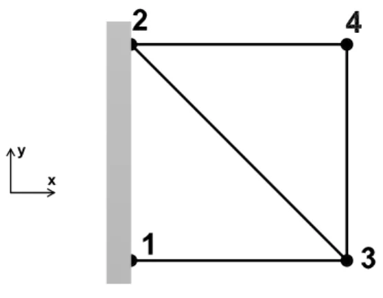
The academic structure that was considered is a planar truss formed of four pin-jointed bars shown in Fig. 1. It is supposed that the external forces and reactions act only on the nodes and result in forces in the bars that are either tensile or compressive. The connections between the structure and the base are assumed to be perfectly rigid. All bars are made of aluminum (E = 72 GPa,ρ = 2700 kg/m3) with a cross-section of 10−4m2.
Figure 1: The 2D truss studied
The only sources of uncertainty that were considered are the ones related to the material stiffness. Therefore, the Young’s modulus of the material of each substructure was assumed to be a random homogeneous quantity such as:
E= E (1 + 0.08η)
withη a uniform random variable defined in the interval [-1;+1]. Table 1 shows the intervals obtained for a probability
P= 99% for the Monte Carlo method and the Lack-Of-Knowledge theory, with 20000 samples generated for the statistical study. The results show great accuracy. It can be noticed that intervals given by the LOK theory are included in the ones
Table 1: 99%-intervals for all the eigenfrequencies of the planar truss for a common uncertainty of 8%
i fi(Hz) Monte Carlo LOK 1 276.42 [266.56 ; 285.82] [266.81 ; 285.63] 2 861.97 [834.27 ; 887.98] [835.85 ; 886.96] 3 1072.5 [1034.40 ; 1108.50] [1035.40 ; 1107.90] 4 1452.4 [1397.10 ; 1506.00] [1398.20 ; 1504.90]
resulting from the Monte Carlo simulations. Recently, Daouk et al. (2013) compared this approach with other methods in the case of small uncertainties. The study of a complex assembly revealed that the LOK theory is accurate and conservative with a significantly low computation cost.
4.3 The need for an extension to large uncertainties
While relations presented in paragraph 4.1 show accurate results in the case of low values of uncertainties, an important question can then be asked whether these relations take into account the presence of large uncertainties. The example shown in Fig. 1 is considered, where the deterministic model has the same characteristics. Nevertheless, the Young’s modulus of the material of each substructure was assumed to be a random homogeneous quantity such as:
E= E (1 + δ η) withδ= �
0.08 for bars 1-3 and 2-3 0.4 for bars 2-4 and 3-4
withη a uniform random variable defined in the interval [-1;+1]. Table 2 shows the intervals for a probability P= 99% for the Monte Carlo method and the LOK theory, where 20000 samples were generated for the statistical study. These
Table 2: 99%-intervals for all the eigenfrequencies of the 2D truss for small and large uncertainties
i fi(Hz) MC LOK
1 276.42 [265.00 ; 287.03] [266.26 ; 286.99] 2 861.97 [752.61 ; 906.16] [807.23 ; 916.14] 3 1072.5 [932.48 ; 1237.80] [893.98 ; 1223.80] 4 1452.4 [1174.50 ; 1700.40] [1165.00 ; 1691.80]
results lead to the conclusion that the approximation in Eq. 4 can not be used to model high values of basic LOKs. The discrepancy seen for some frequencies shows that, in order to accurately consider many large uncertainties in the case of complex industrial assemblies, an extension of the LOK theory is necessary.
5 HIGH VALUES OF UNCERTAINTIES
The uncertain behavior of real industrial structures can seldom be modeled by uncertain parameters with low values. Due to lack of knowledge and the presence of many nonlinearities, high values of uncertainties (≥ 10%) should be consid-ered in order to increase the accuracy and precision of numerical models. Ladev`eze et al. (2006a) introduced an extension of the LOK theory to the case of one large basic LOK, not involving approximations while maintaining a low computation cost. In this paragraph, a generalization of this approach is presented, taking into account a mix of several small and large uncertainties.
Firstly, a family of real and quasi-identical structures is considered. Each structure Ω can be modeled as an assembly of two types of substructures as follows:
• L is the set of l substructures, each associated with small basic LOKs • H is the set of h substructures, each associated with large basic LOKs • Ω = L ∪ H
• /0 = L ∩ H
The approach is based on the consideration that a high value of uncertainty, related to structural stiffness, can be expressed as an addition or subtraction of stiffness to the total stiffness of the assembly, weighted by the value of the LOK. That would have an effect on the dynamical behavior of the assembly. In a practical way, let mH be a large basic
LOK associated with a substructure of H . The objective is to calculate the angular eigenfrequenciesω�i(mH) and the
eigenmodes �Φi(mH) of the whole assembly perturbed by the large uncertainties, where mH = [mH1mH2 . . .mHh]
T are
random samples which contain the random variables{mHk}hk=1, taken from the intervals{[−mH−k; m+Hk]}hk=1⊂ [−1; +1].
Then the actual problem to be solved is to findω�iand �Φisuch that
(K + h
∑
k=1 mHkKHk) �Φi=ω�i2M �Φi (5) where KHkis the contribution of substructure Hkto the stiffness matrix of the global theoretical model. Seeking to keep
the computational cost low, an approximated solution should be determined, instead of solving directly the problem for each value of the sample mH.
In order to reduce the size of the problem, a reduced modal basis is built. From the eigenmodes of the global deter-ministic FE dynamic model, n modesϕ
i are taken to build the basis, where n is the number of modes of interest. After
that, an improvement of the results with this reduced basis is accomplished. Some statical modesψk
i are introduced to the
basis, which are defined for each Hkby the relation:
Kψk
It is important then to eliminate collinear modes and proceed to a normalization of the static modes with respect to the mass matrix. For the sake of simplification, the same number m of static modesψk
i was considered for each substructure
Hk. Thus, the reduced basis of(n + m × h) vectors writes: B = �ϕ 1 . . .ϕ n ψ 1 1 . . .ψ 1 m ψ 2 1. . .ψ 2 m ψ h 1 . . .ψ h m �
The eigenmodes solution of the eigenvalue problem in Eq. 5 are sought as function of the reduced basis, which means:
� Φi= ΦΦΦx + h
∑
k=1 Ψ ΨΨky k= (ΦΦΦ | ΨΨΨ1ΨΨΨ2· · · ΨΨΨh) x y 1 y 2 .. . y h where ΦΦΦ =�ϕ 1. . .ϕ n � and ΨΨΨk=�ψk 1 . . .ψ k m �. The final step is premultiplying the perturbed problem in Eq. 5 by (ΦΦΦ | ΨΨΨ1ΨΨΨ2· · · ΨΨΨs)T, in order to obtain the following reduced problem of size(n + m × h) × (n + m × h):
ω2 1 0 . .. 0 0 ω2 n 0 B1 + h
∑
k=1 mHk � Φ ΦΦTKHkΦΦΦ B2 B3 B4 � x y 1 y 2 .. . y h =ω�i2 x y 1 y 2 .. . y h (6)where the size of blocks B1and B4is(m × h) × (m × h); the size of block B2is n× (m × h), and of B3is(m × h) × n.
They are defined as follows :
B1 = Ψ Ψ ΨT 1KΨΨΨ1 · · · ΨΨΨT1KΨΨΨh Ψ Ψ ΨT2KΨΨΨ1 · · · ΨΨΨT2KΨΨΨh .. . ... Ψ Ψ ΨThKΨΨΨ1 · · · ΨΨΨThKΨΨΨh B2 = � Φ ΦΦTK HkΨΨΨ1 ΦΦΦTKHkΨΨΨ2 · · · ΦΦΦTKHkΨΨΨh � B3 = Ψ Ψ ΨT1KHkΦΦΦ Ψ Ψ ΨT 2KHkΦΦΦ .. . Ψ Ψ ΨT hKHkΦΦΦ B4 = Ψ Ψ ΨT 1KHkΨΨΨ1 · · · ΨΨΨT1KHkΨΨΨh Ψ Ψ ΨT2KHkΨΨΨ1 · · · ΨΨΨT2KHkΨΨΨh .. . ... Ψ Ψ ΨThKHkΨΨΨ1 · · · ΨΨΨThKHkΨΨΨh
In the case of high values of uncertainties, the evaluation of the strain energies is only needed for substructures of L , namely ones associated with small basic LOKs. This is due to the approximation presented in Eq. 4 linking ∆ω2
i to the
strain energies. If L is a substructure of L , then its strain energy is defined as: � eL( �Φi(mH)) = 1 2Φ� T i(KL+ h
∑
k=1 mHkKHk) �ΦiThe evaluation of the effective LOKs on the angular eigenfrequencies is accomplished in the same way as for the case presented in section 4.1. The linearization of ∆ω2
iLOK= ωi2LOK− ω2i around the theoretical deterministic model remains
correct for the substructures of L , and this is done through the strain energies. For the substructures of H , namely the ones associated with large basic LOKs, the differenceω�i(mH)2− ω2i is considered as it is without any approximation.
The propagation of the LOK intervals is done by adding the contributions of both types of substructures. Thus, for the angular eigenfrequencies associated with the i-th eigenmode, the lower and upper bounds are given as follows:
−∆ωi2−LOK(θ ) ≤ ∆ω2 i ≤ ∆ωi2+LOK(θ ) with ∆ωi2−LOK(θ ) = 2
∑
L∈L m−L�eL( �Φi(mH)) − (ω�i(mH))2− ω2i) ∆ωi2+LOK(θ ) = 2∑
L∈L m+L�eL( �Φi(mH)) + (ω�i(mH))2− ω2i)After evaluating the probability density functions of the bounds, the effective LOKs ∆ωi2−LOK(P) and ∆ωi2+LOK(P) on the angular eigenfrequency are determined for a given probability P.
Due to the size of this reduced system, the computation time is low. However, it remains costly to find the eigenfrequencies and eigenmodes and evaluate the strain energies for each sample of large basic LOKs mH. For this reason, the values of
�
ωi(mH) and �Φi(mH) are estimated by interpolation, using polynomials or collocation methods.
6 APPLICATIONS AND RESULTS
In case of large uncertainties, the Monte Carlo method and the LOK theory were implemented and used to solve the eigenvalue problem in Eq. (3) for two different assemblies. The only sources of uncertainty that were considered are the ones related to the material stiffness. Therefore, in both following studies, the Young’s modulus of the material of each substructure was assumed to be a random homogeneous quantity such as:
E= E (1 + δ η) withδ= �
0.05 for the substructures of L
0.5 for the substructures of H (7) andη is a uniform random variable defined in the interval [-1;+1]. In the case of the LOK theory, it is then considered that m−E= m+E= δ , which means that the basic LOK mE(θ ) is taken as a uniform random variable in the interval [-δ ;+δ ].
For the statistical studies, 10000 samples were generated once and then used by each method. For each generated sample of Young’s moduli or LOKs, a value of the eigenfrequency of the assembly is calculated. Then the probability density function (PDF) is drawn, except for the LOK theory where only bounds are found. As a common representation enabling a homogeneous comparison, the bounds for the probability P= 0.99 were extracted from the PDFs of the Monte Carlo approach. The results shown in the next paragraphs are presented in the form of intervals that contain 99% of the values of the eigenfrequency related to the studied family of structures.
6.1 Beam assembly
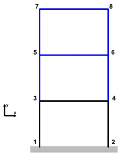
The academic structure that was considered is a planar assembly formed of 9 beams shown in Fig. 2. The connections between the structure and the base are assumed to be perfectly rigid (i.e. nodes 1 and 2 are clamped). The length of the 3 horizontal beams is 1.5 times bigger than the vertical ones. All beams are made of steel (E = 210 GPa,ρ = 7800 kg/m3)
with a circular cross-section of 10−2m2.
Figure 2: The 2D beam assembly used for validation of implementation
Considering the boundary conditions already mentioned, a dynamical analysis without damping was performed in the presence of small and large uncertainties. The focus was on the first three eigenfrequencies of the assembly. Figure 3 shows the shapes of the eigenmodes associated with the considered eigenfrequencies for the deterministic reference struc-ture. All are bending modes. As presented in Fig. 2, the beams colored in blue were associated with large uncertainties
(a) Mode 1: 18.06 Hz (b) Mode 2: 61.27 Hz (c) Mode 3: 114.75 Hz
Figure 3: The shapes of the first three eigenmodes of the deterministic 2D beam assembly Table 3: 99%-intervals for the first three eigenfrequencies of the 2D beam assembly
i fi(Hz) Monte Carlo LOK 1 18.06 [15.93 ; 19.11] [16.74 ; 18.87] 2 61.27 [53.25 ; 66.41] [55.03 ; 65.83] 3 114.75 [98.16 ; 125.43] [101.71 ; 124.08]
(∈ H ), and the others are associated with low values of uncertainties. Thus the corresponding values of uncertainties are given by Eq. (7). Table 3 shows the intervals for a probability P= 99% for the Monte Carlo method and the LOK theory. This academic example was used to validate the implementation of the LOK theory in case of multiple large basic LOKs. The 99%-intervals presented in Tab. 1 are nearly identical, which might be expected given the simplicity of the structure. However, it is interesting to notice that intervals given by the LOK theory are included in the ones resulting from the Monte Carlo simulations. This induces higher precision at a much lower computation cost. An important question can then be asked whether the same accuracy can be obtained when considering a larger assembly, representative of a real industrial structure. The next study aims to provide an answer in this matter.
6.2 Complex 3D assembly
In order to assess the accuracy of the extension of the LOK theory presented previously, it is necessary to study a case representative of a real complex structure. Figure 4 shows the model that was inspired from the geometry of the booster pump studied in the framework of the international benchmark SICODYN (Audebert (2010), Audebert and Fall-Lo (2013)). The main goal of this benchmark was to measure the effective variability on structural dynamics computations and then quantify the confidence in numerical models used either in design purpose or in expertise purpose and finally to ensure robust predictions, that is with a difference between prediction and actual response which is within an accept-able range including all uncertainties. The studied structure is an assembly of a cone and a tube with a wedge between these two elements. The whole set is made of steel (E = 210 GPa,ρ = 7800 kg/m3). The largest side of the cone is clamped.
Figure 4: Mesh of the studied 3D assembly
The characteristics of the different parts of this assembly are presented in Tab. 4 in terms of geometry and FE discretiza-tion. Considering the boundary conditions already mentioned, a dynamical analysis without damping was performed in
Table 4: Characteristics of each part of the 3D assembly
Part Length (m) Interior Radius (m) Thickness (m) Number of FE DOFs Cone 0.4 0.1 / 0.2 0.002 1620 9936
Tube 0.4 0.1 0.01 1584 9720
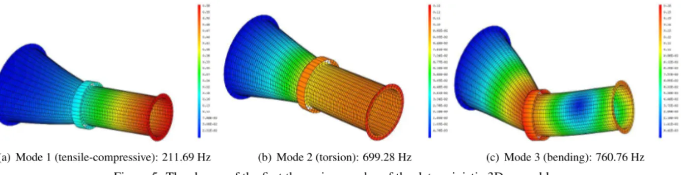
the presence of low and high values of uncertainties on the Young’s moduli of the substructures. As for the previous assembly studied, only the first three eigenfrequencies of the assembly were evaluated in the deterministic and stochastic cases. Figure 5 shows the shapes of the eigenmodes associated with the considered eigenfrequencies for the deterministic reference structure.
(a) Mode 1 (tensile-compressive): 211.69 Hz (b) Mode 2 (torsion): 699.28 Hz (c) Mode 3 (bending): 760.76 Hz
Figure 5: The shapes of the first three eigenmodes of the deterministic 3D assembly
In this case, the cone was the only structure associated with low uncertainties (∈ L ) and the tube and the wedge were the substructures forming H . Thus the corresponding values of uncertainties are given by Eq. (7). Table 5 shows the intervals for a probability P= 99% for the Monte Carlo method and the LOK theory.
Table 5: 99%-intervals for the first three eigenfrequencies of the 3D assembly
i fi(Hz) Monte Carlo LOK 1 211.69 [201.66 ; 219.52] [202.46 ; 217.57] 2 699.28 [658.61 ; 722.94] [662.44 ; 720.19] 3 760.76 [715.42 ; 789.43] [717.11 ; 785.69]
The 99%-intervals given by the LOK theory show little discrepancy compared to the ones given by Monte Carlo simulations. Nevertheless, the LOK theory remains conservative, even in the presence of high values of uncertainties. In addition, simulations that need days with the Monte Carlo method are performed in minutes using this approach. The more the degrees of freedom of the studied model are numerous, the greater this gap will be. However, as defined previously, probability density functions of the response can not be assessed using the LOK theory. Despite that and its intrusiveness, this modeling technique might seem of great interest to engineers. The LOK theory presents some challenges in the implementation because the evaluation of the strain energies is necessary to obtain the effective LOKs of the output of interest. This is added to the construction of the basis, the projection phase necessary to build the reduced problem, and the interpolation of the eigenfrequencies and the eigenmodes. The low computational cost of this technique remains one major advantage.
7 CONCLUSION
Uncertainty quantification is more and more getting the attention of engineers that wish to improve the predictability and robustness of numerical models. This paper aimed to present an interesting modeling technique, called the LOK the-ory, and assess its ability to evaluate the propagation of low and high values of uncertainties through dynamical models. In fact, the Monte Carlo method is non-intrusive and can easily take into account large uncertainties but the computation cost is significantly expensive. That is why modeling techniques The study of an academic planar truss of four bars showed that accurate results can be obtained in the case of small uncertainties, while an extension of the approach is needed in order to take into account large uncertainties. A first comparison with the Monte Carlo method was accomplished in the case of a simple planar beam assembly. The results lead to the validation of the implementation of the technique, consid-ering numerous small and large uncertainties related to structural stiffness. Another comparison was done on a complex assembly representative of a real industrial structure. For this structure too, the Lack-Of-Knowledge theory seems to be conservative, meaning that the resulting intervals are always included in the intervals given by the Monte Carlo simula-tions, which induces higher precision. Unlike the other uncertainty propagation methods, this modeling technique only provides a stochastic interval that bounds the response without any further information about it. Probability density func-tions of the response can not be assessed using the LOK theory. The main advantage of this method is the globalization of all sources of uncertainties, related to data and model, which reveals to be very handy for modeling real industrial assemblies, for low and high values of uncertainties.
In the framework of the SICODYN Project (Audebert and Fall-Lo (2013)), initiated in 2012 and to be carried out till 2015, the LOK theory considered in this paper will be evaluated in the case of a one-stage booster pump of thermal units studied within its industrial environment. Comparisons with other methods will be accomplished, in addition to comparisons with results of the total numerical variability observed in the framework of the benchmark SICODYN. One of the main goals is to evaluate the ability of the LOK theory, to quantify, not only data (parameter) uncertainties, but also model uncertainties, in the cases of low and high values of uncertainties.
8 ACKNOWLEDGEMENTS
This work has been carried out in the context of the FUI 2012-2015 SICODYN Project (pour des Simulations cr´edibles via la COrr´elation calculs-essais et l’estimation d’incertitudes en DYNamique des structures). The authors would like to gratefully acknowledge the support of the FUI (Fonds Unique Interminist´eriel).
REFERENCES
Audebert, S. (2010). SICODYN international benchmark on dynamic analysis of structure assemblies: variability and numerical-experimental correlation on an industrial pump. Mechanics & Industry, 11(6):439–451.
Audebert, S. and Fall-Lo, F. (2013). Uncertainty Analysis on a Pump Assembly using Component Mode Synthesis. In
Proceedings of 4th ECCOMAS Thematic Conference on Computational Methods in Structural Dynamics and Earth-quake Engineering, COMPDYN, Kos Island, Greece.
Chatterjee, A. (2000). An introduction to the proper orthogonal decomposition. Current science, 78(7):808–817. Daouk, S., Louf, F., Dorival, O., Champaney, L., and Audebert, S. (Submitted in 2013). Modelling of uncertainties on
industrial structures : a review of basic stochastic and other methods, and application to simple and complex structures.
Mechanics& Industry.
Fishman, G. S. (1996). Monte Carlo: Concepts, Algorithms and Applications. Springer-Verlag.
Ghanem, R. G. and Spanos, P. D. (1991). Stochastic Finite Elements: A Spectral Approach. Springer-Verlag.
Kleiber, M. and Hien, T. D. (1992). The stochastic finite element method : basic perturbation technique and computer
implementation.John Wiley & Sons, England.
Ladev`eze, P. (2002). On a Theory of the Lack of Knowledge in Structural Computation. Technical Note SY/XS 136 127,
EADS Launch Vehicles, in French.
Ladev`eze, P., Puel, G., and Romeuf, T. (2006a). Lack of knowledge in structural model validation. Computer Methods in
Applied Mechanics and Engineering, 195:4697–4710.
Ladev`eze, P., Puel, G., and Romeuf, T. (2006b). On a strategy for the reduction of the lack of knowledge (LOK) in model validation. Reliability Engineering & System safety, 91:1452–1460.
Le Maˆıtre, O. P. and Knio, O. M. (2010). Spectral methods for uncertainty quantification: with applications to
computa-tional fluid dynamics. Springer.
Louf, F. and Champaney, L. (2013). Fast validation of stochastic structural models using a PGD reduction scheme. Finite
Elements in Analysis and Design, 70–71:44–56.
Louf, F., Enjalbert, P., Ladev`eze, P., and Romeuf, T. (2010). On lack-of-knowledge theory in structural mechanics.
Comptes Rendus M´ecanique, 338(7-8):424–433.
Matthies, H. G., Brenner, C. E., Bucher, C. G., and Guedes Soares, C. (1997). Uncertainties in probabilistic numerical analysis of structures and solids-Stochastic finite elements. Structural safety, 19(3):283–336.
Moens, D. and Hanss, M. (2011). Non-probabilistic finite element analysis for parametric uncertainty treatment in applied mechanics: Recent advances. Finite Elements in Analysis and Design, 47(1):4–16.
Muhanna, R. L. and Mullen, R. L. (2001). Uncertainty in mechanics problems-interval-based approach. Journal of
Engineering Mechanics, 127(6):557–566.
Nouy, A. (2010). A priori model reduction through proper generalized decomposition for solving time-dependent partial differential equations. Computer Methods in Applied Mechanics and Engineering, 199(23):1603–1626.
Ryckelynck, D., Chinesta, F., Cueto, E., and Ammar, A. (2006). On the a priori model reduction: Overview and recent developments. Archives of Computational Methods in Engineering, 13(1):91–128.
Schu¨eller, G. (2001). Computational stochastic mechanics – recent advances. Computers & Structures, 79:2225–2234. Xiu, D. and Karniadakis, G. E. (2003). A new stochastic approach to transient heat conduction modeling with uncertainty.
International Journal of Heat and Mass Transfer, 46(24):4681–4693.
Yamazaki, F. and Shinozuka, M. (1988). Stochastic finite element analysis: an introduction. In Ariaratnam, S., Schu¨eller, G., and Elishakoff, I., editors, Stochastic Structural Dynamics: Progress in Theory and Applications, pages 241–291. Elsevier Applied Science, England.
RESPONSIBILITY NOTICE