HAL Id: hal-01663967
https://hal.archives-ouvertes.fr/hal-01663967
Submitted on 13 Mar 2018
HAL is a multi-disciplinary open access
archive for the deposit and dissemination of
sci-entific research documents, whether they are
pub-lished or not. The documents may come from
teaching and research institutions in France or
abroad, or from public or private research centers.
L’archive ouverte pluridisciplinaire HAL, est
destinée au dépôt et à la diffusion de documents
scientifiques de niveau recherche, publiés ou non,
émanant des établissements d’enseignement et de
recherche français ou étrangers, des laboratoires
publics ou privés.
PIERRE BONNAL
1*, DIDIER GOURC
2, ARI-PEKKA HAMERI
3and GERMAIN LACOSTE
41
CERN, CH1211 Geneva 23, Switzerland 2
ENSTIMAC, F81013 Albi, France 3
UNIL-HEC, CH1015 Lausanne, Switzerland 4
ENIT, F65016 Tarbes, France
Received 16 July 2003; accepted 26 November 2004
For some specific types of construction projects, the classical CPM or PDM scheduling techniques are not the most suitable. Few specific scheduling approaches have been developed to cope with construction projects that are made of either repetitive activities or activities with linear developments. But real-world construction projects do not consist only of such activities. They are generally made of a mixture of linear and/or repetitive activities and of more conventional activities. To allow this, the linear scheduling problem is reformulated, so classical schedule calculation approaches can be used. The implementation of some Allen’s algebra features to avoid adverse discontinuities and to allow crew/work continuity, together with a resource-driven and space-constrained scheduling are among the key features of the proposed approach. It is also a spin-off of off-the-field practices used for scheduling real projects in the particle accelerator construction domain; an excerpt from such a construction project is provided for illustrating the methodology.
Keywords: Construction scheduling, linear scheduling, optimization
Introduction
Over the last two decades, several articles (Selinger, 1980; Johnston, 1981; Chrzanowski and Johnston, 1986; Handa and Barcia, 1986; Russell and Caselton, 1988; Eldin and Senouci, 1994, 2000; Harmelink and
Rowings, 1998; Harmelink, 2001; Moselhi and
Hassanein, 2003) have been published to address the scheduling problem of construction or installation projects which typically have a linear development. Most of these papers refer to the so-called Linear Scheduling Model (LSM) that is an alternate metho-dology to the 40-year-old Critical Path Method (CPM). The linear scheduling methods that are presented in these papers do not allow considering systematically resources except the spatial one. In the present article, we have reformulated the problem so it can be treated as a resource-constrained project scheduling problem. Repetitive construction schedul-ing problems are a class of problems similar to those that can benefit from the LSM approach; the approach
presented in the present article can also be seen as a generalization of the repetitive construction scheduling to the linear scheduling.
The projects concerned by the LSM methodology are projects that consist of a majority of linear activities. Harmelink and Rowings (1998) give the following definition to the latter: linear activities are those activities that are completed as they progress along a path. For instance, the digging of a railway tunnel, the repaving of a motorway or the installation and interconnection works of a particle accelerator, are typically projects that belong to the family of linear development projects.
The implementations of LSM-like approaches on real life projects have demonstrated their efficiency. From a practitioner point of view, the benefits of using the approach stem from:
N
a smaller breakdown of activities is sufficient to perform the activity network analysis; andN
the schedules issued are more concise, whichimprove communication.
Among the scheduling approaches suited to a particular class of construction project, one should also mention
*Author for correspondence. E-mail: [email protected]
Construction Management and Economics
ISSN 0144-6193 print/ISSN 1466-433X online # 2005 Taylor & Francis http://www.tandf.co.uk/journals
In terms of development, repetitive scheduling approaches have certainly reached a higher level of maturity. Several successful attempts have been made to make schedule analyses systematic: CPM-like
calculation with forward and backward passes,
resource-driven scheduling (Moselhi and El-Rayes, 1993; Russell and Wong, 1993; Suhail and Neale, 1994; El-Rayes and Moselhi, 1998; El-Rayes, 2001; Leu and Hwang, 2001; El-Rayes et al., 2002). LSM approaches have not yet benefited of such functional-ities; LSM schedule calculations are often limited to graphical analyses.
As mentioned by El-Rayes (2001), scheduling of repetitive construction projects can be significantly improved by considering three main practical require-ments. These requirements are (1) the application of resource-driven scheduling that enable crew/work continuity, (2) the minimization of the project duration by an optimized utilization of the resources available, and (3) the integration in a single activity network of activities on different types: repetitive and non-repetitive activities for instance.
The aim of the present article is to describe a scheduling methodology that is suitable to projects that have activities with linear developments, and that integrates the three practical requirements mentioned here before. To do so, the problem has been formulated in such a way resource-constrained scheduling metho-dologies can be implemented. Several types of activities are supported: activities that are space-constrained can be mixed with activities that are not; activities with a linear development can be mixed with discrete activi-ties. Some Allen’s algebra features (Allen, 1983) are implemented for addressing the crew/work continuity issue that is also mentioned here before.
The scheduling methodology presented in this article is henceforth called LDSM (Linear-Discrete Scheduling Model) for distinguishing it among the many scheduling techniques that are available for addressing this type of construction problem.
The rest of the article is organized in the following way: definitions are given in section 2. Then an
constrained activities are activities for which spatial resources do not need to be considered to have them scheduled, and then executed. In the framework of such construction project, space-constrained activities are in general the construction/installation activities carried out on the construction site (excavation works, digging works, pipe works, cable pulling, etc.) while non-space-constrained activities are those performed offsite (engineering works, etc.) or at supplier or contractor premises (prefabrication, etc.).
Linear vs. discrete-space-constrained activities Linear space-constrained activities have been defined here before: these are activities that progress along a path; they generally use this ‘path’ a renewable resource, e.g. the digging of a railway tunnel, the paving of a motorway, etc. Discrete-space-constrained activities are activities that also use a spatial renewable resource, but that do not progress along a path, e.g. the digging of a small alcove in a railway tunnel, the earthwork for a junction at the crossing of two motorways, etc.
Linear-discrete schedule diagramming
Above all, schedules are communication media even if the underlying optimization mechanisms are of prime importance. Gantt charts are known to be the best means for communicating the temporal information of a project made of non-space-constrained activities. On these charts, the time goes along the horizontal axis from left to right, while the Work Breakdown Structure (WBS) depicting in a hierarchical way all the activities to perform to complete the project is viewed vertically. Authors of LSM have preferred the one-dimensional space resource viewed over the horizontal axis, while the time runs along the vertical one.
For convenience, and especially for facilitating the communication of LDSM schedules among people certainly more familiar with Gantt charts, the Gantt’s scheme is preferred: the time running along the
horizontal axis and the one-dimensional space stations spread along the vertical axis.
For compactness and for complying with LSM principles, also shared by the critical chain approach
(Newbold, 1998), several non-overlapping activities can be merged on a same row. Both space-constrained activities and non-space-constrained activities are segregated into distinct horizontal strips.
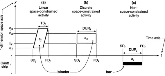
Figure 1 The three types of activities LDSM incl. naming conventions
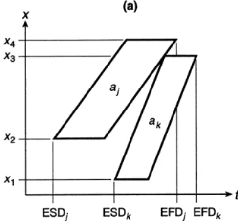
Figure 2 Optimally calculated vs. CPM calculated LDS diagram – example no. 1
The typology of LDSM activities
Basically, LDSM supports three types of activities:
N
linear space-constrained activities,resource-constrained or not;
N
discrete space-constrained activities,resource-constrained or not; and
N
and other activities, discrete, non-space-constrained, resource-constrained or not.In the LDSM vocabulary, all space-constrained activ-ities are called blocks, while others are called bars, in reference to bar charts, a name used for Gantt charts (cf. Figure 1). Blocks can be of two types: parallelo-gram-shaped blocks referring to linear activities and
Figure 4 CPM calculated LDS diagram – example no. 2
rectangle-shaped blocks that correspond to discrete activities.
Linear space-constrained activities (cf. Figure 1a) Let ajbe a linear space-constrained activity, in addition
to precedence and resource constraints, such an activity is characterized by a 6-tuple (xj1, xj2,hj, TSj,Cj21, rj)
with:
xj1: start station of activity aj xj2: finish station of activity aj hj: production rate of activity aj
TSj: temporal span associated with activity aj Cj21: set of predecessors of activity aj; andCj215Ø if ajhas no predecessor
rj: vector of the resources required for completing activity aj.
The production ratehjis the spatial progress foreseen
per unit of time: typically, production rates can be
expressed in feet/hour, km/week, units/day… hj is
positive if ajprogresses along x ascending, i.e. if xj1,xj2;
otherwise hj is negative. The true production rate
capacity is based on |hj| and not onhj.
If the start date SDj of activity aj is known, the
finish date FDj of this activity can be obtained as
follows:
FDj~SDjz xj2{xj1
! "#
hjzTSj: ð1Þ
It is also important to remark that the definition to predecessor activity in the LDS context differs to the one of predecessors in a CPM context. To illustrate this, let aj and ak be two discrete activities, such as
Cj215{aj}. In a CPM context, this means that ak
cannot start until aj has ended. In the LDS
environ-ment, precedence constraints generally means that an activity can start, as soon as its predecessor activities has ended in the vicinity of its start station.
Figure 6 Forward pass DG of example no. 1
Figure 7 Backward pass DG of example no. 1
Discrete space-constrained activities (cf. Figure 1b)
Such an activity is also characterized by a 6-tuple (xj1,
xj2, ‘, DURj, Cj21, rj) with:
xj1: start station of activity aj xj2: finish station of activity aj
DURj: duration of activity aj: DURj5FDj2SDj Cj21: set of predecessors of activity aj; andCj215Ø if ajhas no predecessor
rj: vector of the resources required for completing activity aj.
A discrete constrained activity is a linear space-constrained activity to whichhj5‘ and TSj5DURj. In
the remaining of this article, we won’t make any distinction anymore between linear and discrete space-constrained activities. They will be simply called block activities.
Non-space-constrained activities (cf. Figure 1c) In addition to precedence and resource constraints, the duration is sufficient to describe a non-space-con-strained activity, henceforth called as bar activity. Calculated dates
The aim of a critical path analysis is to determine for all the activities of a network the earliest and latest start and finish dates: ESDj, EFDj, LSDj and LFDj. The
critical activities are those for which earliest and latest dates are identical, i.e. ESDj5LSDj or EFDj5LFDj.
CPM, LSM and LDSM do share the same objective.
An approach for solving a LDS problem
Several approaches can be found to solve a LDS problem. We take two examples to find out where the solving difficulties are located.
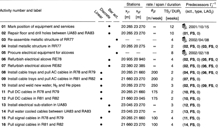
Figure 10 Example-description of the activities
Example no. 1
Let aj and ak be two block activities such as aj5(x4,x2,hj,TSj,Ø,Ø) and ak5(x1,x3,hk,TSk,{aj}, Ø),
with x1,x2,x3,x4, i.e. hj,0 and hk.0. Figure 2a
shows how these two activities should be scheduled optimally, i.e. as soon as possible. It can be observed that the early finish date EFDjof activity ajis scheduled
later than the early start date ESDk of activity ak.
Figure 2b shows how CPM would have scheduled these two activities.
The approach we are proposing in this article for solving such a problem requires a systematic fragmen-tation of the space-constrained activities along the space axis. This means for instance that activities aj and ak would be broken down into four sub-activities aj9,
aj0, ak9 and ak0 such as: aj95(x4, x3,hj, TSj, Ø, Ø),
aj05(x3, x2,hj, TSj, {aj9} Ø), ak95(x1, x2,hk, TSk, Ø, Ø), ak05(x2, x3,hk, TSk, {ak9,aj0}, Ø) (see Figure 3a).
The precedence constraints of this set of sub-activities are the following: aj9 $ aj0, ak9 $ ak0 and
aj0$ ak0 (the ‘x $ y’ stands for ‘x precedes y’). The
results of a CPM calculation are given in Figure 3b. In some situations, such schedule can be acceptable. But in most real-world situations, project management practitioners would prefer a continuity in the perform-ing of activity ak, i.e. baselining LSDk9 and LFDk9
instead of ESDk9 and EFDk9. Implementation of
features of Allen’s temporal logic relation leads to a calculation procedure that fulfills real-world require-ments, especially the possibility of mixing earliest and latest dates when needed, and by the way responding to the crew/work continuity requirement.
Example no. 2
Let ajand akbe two activities such as aj5(x2, x4,hj, TSj,
Ø, Ø) and ak5(x1, x3, hk, TSk, {aj}, Ø), with
x1,x2,x3,x4, i.e.hj.0 and hk.0.
Three cases shall be distinguished: hj,hk (cf.
Figure 4a),hj.hk(cf. Figure 4b) or hj5hk. In all cases,
akmust be scheduled so it just does not interfere with
if hj>hk:
SDk00~SDj0zTSj ð4Þ
FDk00~FDj0zTSkz xð 3{x2Þ#hk{ xð 3{x2Þ#hj ð5Þ
Extended set of precedence constraints
In his temporal algebra, Allen (1983) has proposed eight relations (and 13 if their inverses are considered) for describing all the possible configurations of two temporal intervals. These 13 relations are presented in Figure 5.
The four types of precedence constraints of the precedence method can be defined using Allen’s formalism as follows (let aj and ak be two activities;
symbol~ stands for ‘or’):
Let aj and ak be two space-constrained activities, the
Allen’s temporal logic relations that best describe the precedence constraints featured in a fragmented LDS diagram are:
Equivalent date graph
The use of a date graph (DG) – or point graph (Zaidi, 2001) – is convenient to solve an activity network that involves Allen’s temporal logic relations. A date diagram is a valued digraph in which nodes (vertices) feature the dates to calculate – also called time stamps in some textbooks and articles – and arcs (edges) the time intervals that separate dates that are directly dependent.
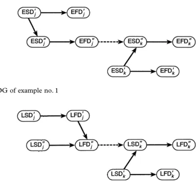
negative intervals, i.e. the arcs that correspond to basic constraints of the precedence method. Two types of DGs are required to solve this problem: a forward pass DG that is used for calculating early start dates, and a backward pass DG for calculating latest dates. Figure 6 gives the forward pass DG that corresponds to example no. 1, and Figure 7 gives the backward pass DG of the same DS diagram. On both DGs, the dashed arc between FDj0 and SDk0 depicts a
weak interval, while all other arcs are representing strong intervals.
Date calculations
The calculations of the dates of such a date graph are straightforward. This can be performed in three steps. Step 1
The graph is broken down into sub-graphs by eliminating temporarily all weak arcs (cf. Figure 8). All the resulting sub-graphs should be irreflexive (self-loop free) and acyclic. A sub-graph G is said to be antecedent to a sub-graph G’, if a weak interval, mapping from G to G’ has been removed.
Step 2
Early date calculation (forward pass) starts in the sub-graphs that have no antecedent sub-graph, and within these sub-graphs, on the node that has no incoming arc. The early start date of the project (ESDproject) is
assigned to these very first nodes. Formulas such as (1) are then used for propagating calculations in a given sub-graph.
Step 3
When all the dates are calculated in a given sub-graph, propagation can continue over weak intervals. To do that, CPM principles are applied. This is repeated until all the dates are calculated.
In a given sub-graph, backward calculations may sometimes be required for time stamping some of its nodes. This is the case for instance of ESDk9 of example
given in the present section.
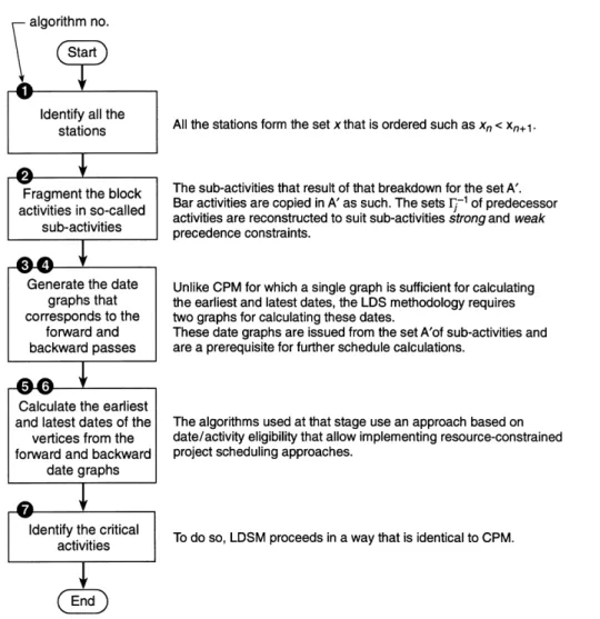
Seven algorithms need to be run successively to solve a LDS problem. A set of activities including their precedence and resources constraints is sufficient to describe the problem. Algorithm no. 1 aims at finding all the stations associated with the space-constrained activities. Algorithm no. 2 fragments the activity net-work into sub-activities. Algorithms nos. 3 and 4 generate the forward and backward pass DGs. Algorithms nos. 5 and 6 calculate, respectively, earliest and latest dates of sub-activities. Finally, algorithm no. 7 identifies the critical sub-activities.
For the sake of simplicity, these algorithms are
presented in a pseudo-code form. Symbols ‘ and ~
stand respectively for ‘and’ and ‘or’; statement ‘arb’ means ‘assign b to a’.
Let A be the set of all the activities of the project; each activity aj is defined as in section 2. Let
X be the set of all the stations xj associated with this
problem.
Algorithm no. 1: identification of the stations
Algorithm no. 2 provides a tool for fragmenting all the block activities into sub-activities. Bar activities are just duplicated into this new set. Let A’ be the set of all the sub-activities of the project.
Note: The set Cj21of the predecessors of an activity aj
is made of 3-tuples made of:
Explanations
Line 30 scans all the activities of A in an ordered way given by line 20. For block activities, two cases are
considered: either h.0 (line 40) or h,0 (line 110).
Lines 50 and 120 scan in an ordered way all the stations spread all along the block activity that is being processed. This means that such an activity is broken down into as many sub-activities as there are inter-mediate stations between the activity’s start and finish stations. P and Q are temporary sets that are used for identifying all the predecessors of the sub-activity that is scrutinized. The following rule is used for
block type is looked at through their corresponding sub-activities. A precedence constraint is set up between possible predecessor sub-activities and the sub-activity that is being processed if the start and end stations are matching. This is the purpose of the last statement of (lines 70 and 140). The first two lines of these statements aim at addressing the problem presented with example no. 2.
Once the predecessors of a sub-activity are defined, they are appended to the set A’.
Algorithms nos. 3 and 4 are used for generating the
forward and backward pass DGs. Let GF be the
forward pass DG; GF5<DF; IF> where DF is the set
of the earliest dates to be calculated and IFis the set of
4-tuples featuring intervals. These 4-tuples are made of four data items: the extremity nodes/dates, the delay that separates these two dates and the type of interval that can be either strong or weak. Because precedence constraints can be of several types, the predecessor set Cj21of an activity ajis made of triplets (as already seen)
(ak,skj, LAGkj), where akis an immediate predecessor
of aj, skj denotes the type of precedence relation
between akand aj, and LAGkjwhich is used to separate
the finish of akand the start of aj.
Algorithm no. 3: generation of the forward pass DG
strong constraint, it is assigned to IFas from line 150.
Let GBbe the backward pass DG; GB5<DB; IB>. The
generation of this backward pass DG is identical to the one of the forward pass DG given by algorithm no. 3, except the replacement of F indices by B indices,Cj21
byCjand the replacement of lines 140 and 150 by:
Algorithms 5 and 6 provide a way for calculating a date, earliest dates (EDj) for the vertices of the forward pass
DG; latest dates (LDj) for the vertices of the backward
pass DG. Let be the set of the activities that are
scheduled at a given date, and the set of the
activities that are eligible for being scheduled (mainly because their predecessor activities have been sche-duled) at that same date.
calculations within a given activity.
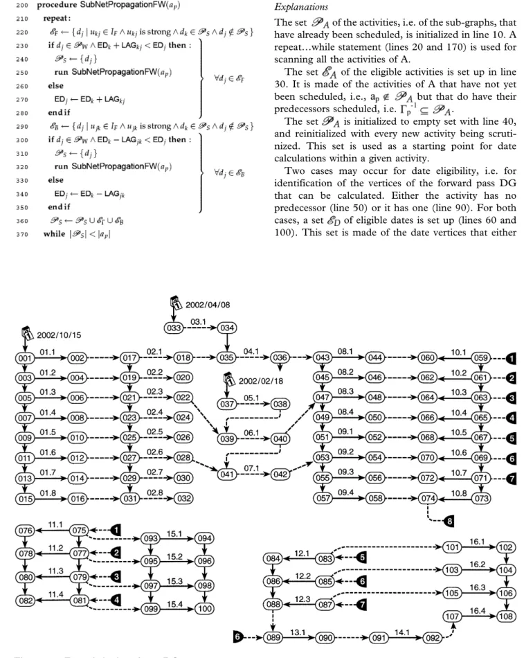
Two cases may occur for date eligibility, i.e. for identification of the vertices of the forward pass DG that can be calculated. Either the activity has no predecessor (line 50) or it has one (line 90). For both cases, a set of eligible dates is set up (lines 60 and 100). This set is made of the date vertices that either
have no in-coming edge (case Cp215Ø) or that have
weak type in-coming edges (caseCp21?Ø). The project
start date is assigned to the earliest date EDj if the
parent activity has no predecessor (line 70); otherwise, it is the latest date among those associated to the date vertices ofCj21that is assigned to EDj(line 110). The
vertex djis then appended to the set (lines 80 and
120).
The date propagation within a given activity/sub-graph requires a unique starting point; this is the
purpose of line 140. When is made of more than
one date, it is the earliest one that is preferred and
appended to .
The procedure SubNetPropagationFW is called for propagating the dates of a given activity/sub-graph (line
150). The sets and are used for identifying
eligible dates (lines 220 and 290), i.e. the dates that are
not yet scheduled ( ) but have adjacent
vertices dk already scheduled ( ). It may
happen that such a date has already been
sche-duled: but . If the newly
calcu-lated EDjis greater than the previously calculated (lines
230 and 300), this latter is superseded by the new one (lines 240 and 310). Otherwise, the procedure SubNetPropagationFW is run again with a new starting point.
Algorithm no. 6: calculation of the latest dates
Finally, algorithm no. 7 calculates the critical activities of the project. The critical activities of an activity network are defined as activities for which earliest dates and latest dates coincide. This means that one cannot delay one of these activities without delaying propor-tionally the completion date of the project.
Explanations
Line 10 picks up a date dp, the earliest, among all the
dates of an activity ap. The total float TFpis calculated
as the difference between the latest and the earliest
near Geneva, Switzerland, uses at co-ordination level a scheduling approach that is very similar to the LDSM. The one used for that project is slightly more complex because it also integrates a line-of-balance mechanism. The LHC will provide particle physics community with a tool to reach the energy frontier above 1 TeV. To deliver 14 TeV proton-proton collisions, it will operate with about 1700 cryo-magnets using NbTi super-conductors cooled at 1.8 K. These cryo-magnets will be installed in the 27-km long, 100-m underground ring tunnel that was excavated 15 years ago for housing the LEP (Large Electron-Positron) accelerator. After a decade of research and development, the LHC main components are being manufactured in industry.
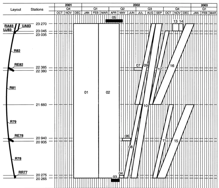
The installation works have started with the refur-bishing of the existing infrastructures. The installation schedule of the LHC project consists of about 2000 work units. The construction of new civil works has started in 1998. The particle physics community expects to have this new accelerator installed and fully commissioned by mid-2007. For the sake of simplicity, we have limited our example to a small sub-set of this large-scale project: the installation of the general services of sectors 7–8 (one-eighth of the main ring). The LHC co-ordination schedule can be seen from www.cern.ch. A summary of this schedule is provided in the Appendix of this paper.
The sub-set used as an example is made of 16 activities, or work units, as referred to in the LHC project jargon. These activities are described in Figure 10, including their duration and predecessors.
Activities 03 and 05 are carried out away from the installation site (i.e. the LHC tunnel). For that very reason, these activities are of bar type. Activities 01 and 02 are activities that require the whole tunnel for being performed; they are of discrete space-constrained type for featuring this characteristic. Activities 04, 06, 07, 13 and 14 are spot activities. They correspond to very specific works to be performed in punctual locations
in the LHC tunnel; few meter lengths of
space-constrained activities; all theirhjhave been set to
positive values in order to provide a pre-optimization of the schedule.
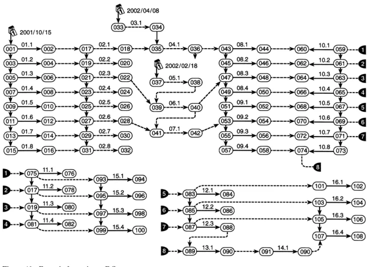
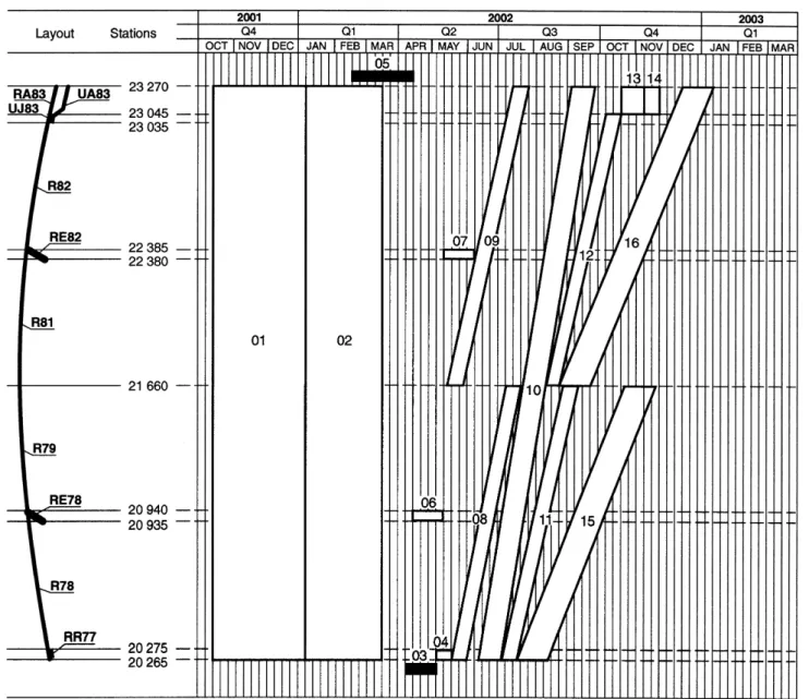
The seven algorithms presented in the previous section have been run on this sub-set of activities; the results of the computations are given in Figures 11–17. The result of algorithm no. 2, i.e. the corresponding sub-activities is given in Fig. 11. The forward and backward pass DGs, as generated using algorithms 3 and 4, are given in Figures 12 and 13. The results of the computations obtained using algorithms 5, 6 and 7 are given in Figures 14 and 15. Two Gantt charts are proposed, one featuring the earliest dates for these 16 activities (Figure 16), another with the latest dates (Figure 17).
Based on this case experience, this approach improves both the analysis of the activity net-work and, because of a better visualization, ease the communication of the schedule. Rescheduling and the dynamic impact of changes can be better understood.
Conclusion
For some specific types of construction projects, specifically the ones that require activities with linear development and/or repetitive activities, the classical project scheduling approaches, based on the CPM or PDM, are not the most suitable. Therefore, few specific approaches were developed to cope with these types of projects; but none of them addresses specifically the mixture of linear type activities together with non-space-constrained activities, in a single resource-driven scheduling system.
With the linear-discrete scheduling model, the linear problem is transformed into a standard resource-contrained project scheduling problem, onto which a wide range of algorithms can be applied, especially those for optimizing the allocation of resources (see, for example, Hartmann, 2001), including the critical chain approach (Newbold, 1998).
One of the key features of the methodology is the implementation of a sub-set of Allen’s temporal
logic relations, used to avoid adverse discontinuities. If we look at the past, activity-on-arrow diagrams were first proposed in the late 1950s, for finding solutions to project activity networks. These
net-works could model only finish–start precedence
constraints. Activity-on-node diagrams offer more flexibility from that point of view: in addition to FS precedence constraints, the project scheduler has the possibility to model SS, SF or FF constraints, with or without lag. The Allen’s temporal logic relations offer 13 additional configurations that can be very useful to project schedulers, especially to those who are in charge of large-scale speculative project schedules, and who have not the possibility to describe thousand of activities. The scheduling
of space-constrained projects are among the ones that can benefit from using precedence constraints mixed with Allen’s relations, but such a scheduling approach can be beneficial to many other project contexts.
Such an integrated method provides project manage-ment practitioners with better means to handle time variation in their tasks. In doing this, it enables project managers to better master overall time usage in the project while at the same time giving them better control to meet project milestones and, most impor-tantly, to reduce project lead-times. Lead-time
reduc-tion correlates with a better quality, a better
productivity, and by the way to projects with higher return on investment.
References
Allen, J.F. (1983) Maintaining knowledge about temporal intervals. Communications of the ACM, 26(11), 832–43.
Ashley, D.B. (1980) Simulation of repetitive-unit construc-tion. Journal of Construction Division, ASCE, 106(2), 185–94.
Chrzanowski, E.N. and Johnston, D.W. (1986) Application of linear scheduling. Journal of Construction Engineering and Management, ASCE, 112(4), 476–91.
Eldin, N.N. and Senouci, A.B. (1994) Scheduling and control of linear projects. Canadian Journal of Civil Engineering, 21(2), 219–30.
Eldin, N.N. and Senouci, A.B. (2000) Scheduling of linear projects with single loop structures. Advances in Engineering Software, 31, 803–14.
El-Rayes, K. (2001) Object oriented model for repetitive construction scheduling. Journal of Construction Engineering and Management, ASCE, 127(3), 199–205.
El-Rayes, K. and Moselhi, O. (1998) Resource-driven scheduling of repetitive activities. Construction Manage-ment and Economics, 16(4), 433–46.
El-Rayes, K. and Moselhi, O. (2001) Optimizing resource utilization for repetitive construction projects. Journal of Construction Engineering and Management, ASCE, 127(1), 18–27.
El-Rayes, K., Ramanathan, R. and Moselhi, O. (2002) An object-oriented model for planning and control of housing construction. Construction Management and Economics, 20(3), 201–10.
Handa, V. and Barcia, R. (1986) Linear scheduling using optimal control theory. Journal of Construction Engineering and Management, ASCE, 112(3), 387–93.
Management, ASCE, 111(3), 308–23.
Leu, S. and Hwang, S. (2001) Optimal repetitive scheduling model with shareable resource constraint. Journal of Construction Engineering and Management, ASCE, 127(4), 270–80.
Moselhi, O. and El-Rayes, K. (1993) Scheduling of repetitive projects with cost optimization. Journal of Construction Engineering and Management, ASCE, 119(4), 681–97. Moselhi, O. and Hassanein, A. (2003) Optimized scheduling
of linear projects. Journal of Construction Engineering and Management, ASCE, 129(6), 664–73.
Management, ASCE, 119(2), 196–214.
Selinger, S. (1980) Construction planning for linear projects. Journal of Construction Division, ASCE, 106(2), 195–205. Suhail, S.A. and Neale, R.H. (1994) CPM/LOB: new
methodology to integrate CPM and Line of Balance. Journal of Construction Engineering and Management, ASCE, 120(2), 667–84.
Zaidi, A.K. and Levis, A.H. (2001) TEMPER: a temporal programmer for time-sensitive control of discrete events. IEEE Transaction on Systems, Man & Cybernetics – Part A, 31(6), 485–96.