Visualization of Frequent Itemsets with Nested Circular Layout and Bundling Algorithm

O

pen

A

rchive

T

OULOUSE

A

rchive

O

uverte (

OATAO

)

OATAO is an open access repository that collects the work of Toulouse researchers and makes it freely available over the web where possible.

This is an author-deposited version published in : http://oatao.univ-toulouse.fr/

Eprints ID : 12929

To link to this article : DOI :10.1007/978-3-642-41939-3_38 URL : http://dx.doi.org/10.1007/978-3-642-41939-3_38

To cite this version : Bothorel, Gwenael and Serrurier, Mathieu and Hurter, Christophe Visualization of Frequent Itemsets with Nested Circular Layout and Bundling Algorithm. (2014) In: International Symposium on Visual Computing - ISVC 2014, 29 July 2013 - 31 July 2013 (Rethymnon, Greece).

Any correspondance concerning this service should be sent to the repository administrator: staff-oatao@listes-diff.inp-toulouse.fr

Visualization of Frequent Itemsets with Nested

Circular Layout and Bundling Algorithm

Gwenael Bothorel1,2_{, Mathieu Serrurier}2_{, and Christophe Hurter}2,3

1

DSNA/DTI, avenue du Docteur Maurice Grynfogel, 31100 Toulouse, France http://www.developpement-durable.gouv.fr/-navigation-aerienne-.html

2

IRIT, 118, route de Narbonne, 31062 Toulouse Cedex 9, France http://www.irit.fr

3

ENAC, 7 avenue Edouard Belin, BP 54005, 31055 Toulouse Cedex 4, France http://www.enac.fr

Abstract. Frequent itemset mining is one of the major data mining issues. Once generated by algorithms, the itemsets can be automati-cally processed, for instance to extract association rules. They can also be explored with visual tools, in order to analyze the emerging pat-terns. Graphical itemsets representation is a convenient way to obtain an overview of the global interaction structure. However, when the com-plexity of the database increases, the network may become unreadable. In this paper, we propose to display itemsets on concentric circles, each one being organized to lower the intricacy of the graph through an op-timization process. Thanks to a graph bundling algorithm, we finally obtain a compact representation of a large set of itemsets that is eas-ier to exploit. Colors accumulation and interaction operators facilitate the exploration of the new bundle graph and to illustrate how much an itemset is supported by the data.

Keywords: Data Mining, frequent itemsets, graph visualization, bundling, optimization.

1

Introduction

Frequent itemsets mining aims at finding links between data, which may not be easily detected. Among the varied fields of Data Mining, it is one of the most studied, because it is a key elements in mining pattern. This is why along two decades, it has been the subject of many studies and publications. For instance, in 1994, Agrawal and Srikant have presented Apriori algorithm which leans on frequent itemsets calculations [1]. Later, other algorithms and methods have been studied, like CAP [2] or DHP [3]. The frequent itemsets can be processed in a next step of automatic calculation, for instance in order to find associations rules. Representing and exploring data mining results is a challenging issue since the number of itemsets or rules can be very large when the complexity of the database increases. The association rules are displayed in systems like AViz, which is an interactive visualization system for discovering numerical association rules from

large data sets [4], or ARVis which shows the rules and associated measures values in a 3D information landscape [5]. But before visualizing association rules, it is also interesting to visualize the frequent itemsets. FIsViz proposes such an approach [6]. It displays the frequent itemsets in a 2D space, by linking the items thanks to connecting edges. Such a tool gives a global graph of the dataset. It illustrates that it is necessary to use a graph when the purpose is the representation of itemsets. Indeed we have to show at the same time the data and the links between the different elements. Moreover, an element is generally involved in many itemsets that can have different sizes. So a graph layout is much adapted to show frequent itemsets. Thus, trying to find frequent itemsets patterns with such a presentation, is trying to find patterns in graph mining. This issue has been recently studied in [7]. It shows that graph mining has become an active and important theme in data mining. One problem is the complexity of the representation, considering the tremendous quantity of connections between the nodes.

As the number of edges can be very large in a graph representation of data, in recent years, graph bundling methods have gained increased attention. They stem from studies on confluent drawing by reducing non-planar graphs to pla-nar ones [8]. The purpose was to allow groups of edges to be merged together and drawn as ’tracks’. Bundling starts with a set of nodes positions, given as input data or computed by a layout algorithm. Edges being close in terms of graph structure, position, data attributes or combinations, are drawn as tightly bundled curves. This trades clutter for overdraw and produces images which are easier to understand and/or better emphasize the graph structure. Blend-ing or shadBlend-ing can be used to add information or emphasize structure [9–11]. Bundling algorithms exist for both compound (hierarchy-and-association) [12] and general graphs [9, 13, 14]. However attractive, many bundling algorithms for general graphs are relatively complex and have high computational costs. A recent study has proposed a faster method based on density maps using kernel density estimations. It relies on graphic cards acceleration techniques [15].

In this paper, we propose to apply a bundling method to a new graph represen-tation of itemsets that takes advantage of their properties (Itemsets are described in Section 2). Itemsets are disposed on nested circles, each one corresponding to the number of items in the itemsets. Then an algorithm reorganizes the itemsets in order to have relevant proximities of the nodes. Finally the bundling algo-rithm is applied. As the proximity of the connections is a key factor indicating that they correspond to frequent itemsets, the bundling simplifies the clutter that becomes more readable (Section 3). Moreover, Infoviz techniques are used to enhance the visualization, particularly by using color and transparency accu-mulation, and interaction operators help the user to explore the bundle layout (Section 4).

2

Frequent Itemsets

Data mining consists in extracting knowledge from a vast volume of data. One purpose is to find relevant patterns that are underlied by this data. A database

is a set of vectors < ai1, ai2, ..., aim >, also known as tuples, over an attributes

space A = {A1, A2, ..., Am}. The attributes are qualitative (string, category,

enumeration) or quantitative items which can be discretized. We denote an item as a value of an attribute (e.g. ai2). An itemset or k-itemset is a subset of values

in the attributes space. k is the number of items concerned by the itemset: k∈ {1, 2, ..., m}.

The database used to illustrate the paper is the Mushroom data set from the UC Irvine Machine Learning Repository1. It includes descriptions of hypothetical samples corresponding to 23 species of gilled mushrooms. The database consists of 8416 tuples of 23 discrete attributes about the edibility, the cap shape, the odor, the ring, the habitat, etc. For instance the cap shape attribute may have curve, flat, bell values, and the odor may have almond, anise, none values. An example of 2-itemsets is {capshape = f lat, odor = anise}.

Itemsets are mainly characterized by the support which indicates the fre-quency they appear in the database (i.e. k-itemset with a frefre-quency equals to 0.3 appears in 30% of the tuples in the database). A frequent itemset is an item-set which has a support greater than a threshold. Obviously, the support of a k-itemset is greater or equal than the support of a (k + 1)-itemset that contains this k-itemset. This (k + 1)-itemset is then named a superset of the k-itemset. So, as the value of k is increased, the support is decreased. As explained in [1], the k-frequent itemsets are iteratively built thanks to the combinations of two (k − 1)-frequent itemsets that differ only on a single item. For instance, the 2-itemset {a, b} is the combination of the 1-itemsets {a} and {b}. The 4-itemset {a, b, c, d} is the combination of the 3-4-itemsets {a, b, c} and {a, b, d}, but it is also the combination of the 3-itemsets {a, b, d} and {b, c, d}, or {a, b, d} and {a, c, d}, etc. This type of approach ensures that all the k-frequent itemsets will be extracted given a support threshold and a maximal value of k.

One major challenge of data mining is the exploration and the analysis of the whole set of frequent itemsets which is usually very large.

3

Circular Graph Layout for Frequent Itemsets

Usually, frequent itemsets presentations are linear layouts as shown in Figure 1. This type of presentation becomes quickly unreadable as the number of nodes and frequent itemsets is increased, and the layout is horizontally stretched to show the whole graph. Moreover, to keep the unicity of each node in order not to clutter up the graph, several frequent itemsets are usually connected to the same nodes. Taking into account the construction of the itemsets, we propose a circular presentation shown in Figure 2. We build our representation in three steps:

1. Structure of the graph

2. Optimization of the itemsets positions 3. Graph bundling

1

Fig. 1.Examples of frequent itemsets linear layout. From [16] (left) and WiFIsViz [17] (right)

Fig. 2. Circular graph presentation of frequent itemsets: construction principle. {A, C, E} is built from {A, C} and {A, E}, which are built from {A} and {C} and from {A} and {E}. {A, C, E} if also built from {A, E} and {C, E}.

Structure of the Graph. The graph is built with concentric circles, separated from the same distance, each one corresponding to the cardinal of the frequent itemsets. The 1-itemsets are on the external circle, the 2-itemsets on the next smaller circle, and so on until the smallest circle corresponding to the frequent itemsets with the highest cardinal. On this circular graph layout, a node is a frequent itemset and the segments are the links between the frequent itemsets of two consecutive circles. An itemset is the combination of two previous itemsets. Note that it can stem from several pairs of previous itemsets (itemset {A, C, E} in Figure 2 for instance). In this case, all the combinations are represented. The distance between the nodes of a same circle is calculated in order to have an homogeneous repartition. Figure 4 shows examples of circular graphs.

Graph layouts with many nodes and edges have always to face the problem of readability due to the cluttering. A way to improve a circular graph layout, with one circle, has been studied in [18].

Optimization.In our study, to enhance the readability of the graph layout, we reorganize the itemsets on the circles, by minimizing the sum s of the segments length. In order to reduce s, we use a simple hill climbing algorithm which finds a local minimum. Two random itemsets are swapped on a random circle. If s is

decreased then this permutation is kept, otherwise it is cancelled. This operation is done a large number of times in order to find a minimum value of s.

Graph Bundling. Graph bundling algorithms aims at simplifying a graph by merging close edges in order to obtain main tracks. We have chosen Kernel Density Estimation-based Edge Bundling [15] for its simplicity and speed. It is simple because it requires only an input graph with nodes positions. It is efficient because GPU processing allows to make it parallelizable and much faster than comparable methods. Considering that each edge links two itemsets of two con-secutive circles, the begin and end points must not be moved. Thus the bundling algorithm must be applied to the partial graphs between two consecutive circles. So, with N circles, it must be applied N − 1 times. The final layout is the combination of the partial bundlings (See Figure 3).

Our representation has many advantages:

• With the optimization, there is a coherence between the itemsets proprieties and their positions. Indeed if the itemsets are linked then they are more likely to be close. Otherwise, they are further.

• Considering the way to build an itemset from previous ones, the combination complexity should always grow as the value of k increases, and become un-readable on a small circle. However, the constraints of the support limit this effect. Indeed the number of itemsets generally increases with the first values of k, and then decreases quickly. In Figure 4(a), there are 11 1-itemsets, then the number of itemsets increases and finally decreases to 8 5-itemsets. • The bundle layout is a way to simplify a complex graph. The optimization

ordering the itemsets, the bundling groups edges that have common item-sets upstream or downstream. Thus the graph is more clear and easier to exploit compared to the original graph. The graph layouts of Figure 4(b) are completely unreadable, as the bundle graph gives information about the itemsets. Indeed with the latter it is easier to discriminate the edges leading to itemsets or leaving them. The whole process of generating the visualiza-tion takes less than two minutes.

• The bundle representation is a way to detect many itemsets proprieties. Indeed it is easier to notice if an itemset has many connections or not, to have an idea of the relations between itemsets. Thus areas where there are many connections correspond to areas where there is much information. This is illustrated in Figures 4 and 5.

4

Itemset Visualization Enhancement

Having built the itemsets circles, given a support threshold, we propose to en-hance the visualization by three ways:

1. Alpha assignment 2. Color accumulation 3. Itemsets selection

Fig. 3. The final bundling is the result of successive partial bundlings between two consecutive circles. Example with four circles.

(a)

(b)

Fig. 4. (a) From left to right: original graph showing frequent itemsets (support=0.5 - number of segments=440 - segments length sum=112). Then the graph is optimized (segments length sum=72). Finally it is bundled. (b) The same sequence with a support equals to 0.45 and 6 circles. There are 1776 segments and the segments length sums are respectively 443 and 303.

Alpha Assignment. In order to emphasize the most relevant itemsets (i.e. the ones with greater support), we propose to use the support as the alpha trans-parency value. As the support concerns only the itemsets, that is to say the begin and end points of each edge, the value of the transparency gradients on the edges corresponds to the interpolation of the supports between these two points. It allows to have a continuous gradient of transparency, and that facili-tates the layout overview.

(a) (b)

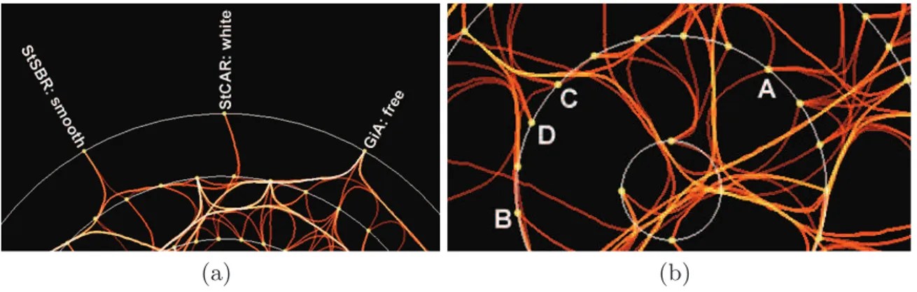
Fig. 5.(a) The accumulation of the color and the transparency is stronger on the right 1-itemset than on the others. It corresponds to a higher support. (b) Points C and D are maximal itemsets, whereas A and B are not.

Fig. 6. Different types of selections. Left: as a 1-itemset is selected, the propagation shows which itemsets stem from this itemset. Middle: the selection of a 1-itemset is disseminated to the supersets, and from these 2-itemsets to the 1-itemsets. It shows which attributes share the same itemsets than a chosen attribute. Right: brush selection of edges. It shows which itemsets are affected by this selection.

Color Accumulation. Another way to get information about the itemsets is to use accumulation. This technique is a consequence of edge bundling, because the bundling distorts the original segments to get bent overlaid edges. So, the more segments are involved in a bundle edge, the more accumulation there is, and it enhances the values of the color and the transparency. As a result the value of the support has a direct effect on the visibility and the color of the edges. Thus, a itemset with a high support appears with a high color level and a high opacity. This feature makes it easier to enhance the most itemsets that are involved in the database, and to reduce the others.

Figure 5(a) illustrates these points. The RGBA value of the color is (1.00, 0.31, 0.21, 0.66). The right itemset corresponds to the attribute Gill attachment = free. It appears 8200 times in the database (support=97.4%), and has 11 su-persets. As these values are large, the resulting accumulation of green and blue reaches 1.0, and it is the same for alpha. So the resulting color of the edges leaving this 1-itemset is (1.0, 1.0, 1.0, 1.0), which corresponds to white color

without transparency. Moreover, the edge leaving leftward is white, whereas the edge leaving rightward is yellow. It indicates the area of the second circle where the 2-itemsets are more concerned by this 1-itemset, and where they are less con-cerned. The left itemset of Figure 5(a) corresponds to the attribute Stalk surface below ring = smooth. It appears 5076 times in the database (support=60.3%), and has 4 supersets. The visual aspect of the edges leaving this itemset shows that its support is lower and that it has fewer supersets than the right itemset. Indeed, the green component is quite low and the blue value is lower. So the resulting edge is orange, with some transparency. In Figure 5(b) we can eas-ily remark that C and D have no supersets. This kind of remarkable itemset is known as maximal itemset. Such an itemset is especially valuable in data mining process. On the contrary, we can immediately deduce from the visualiza-tion that A and B are not maximal itemsets since they have at least one superset. Itemsets Selection. In order to focus on one or more itemset we propose a selection tool. Selecting an itemset shows only its backward and forward con-nections, thanks to a propagation effect, while the other connections are hidden. Thus selecting the itemset A on Figure 2 highlights its connections to AC and AE, and from AC and AE to ACE. Selecting AC highlights its connections to A, C and ACE, and selecting ACE highlights its connections to AC, AE, CE, and then to A, C and E. Figure 6 shows an examples of this selection. On the left picture, the selection of the itemset Gill spacing=close (support = 81.1%) shows that it has five supersets on level 2. The propagation to the next levels gives seven, four and finally one itemset. Note that, as the algorithm (see Section 3) gathers the itemsets in the same areas, they are not spread on the graph.

It is also interesting to know for instance which 1-itemsets share the same 2-itemsets than the 1-itemset that is selected. A backward feature proposes to highlight differently these 1-itemsets, with a simple green color coding. So, by selecting a 1-itemset, there is a propagation to the supersets, and then to the other 1-itemsets that are previous itemsets of these supersets. As a consequence, when a 1-itemset is selected, it is easy to detect the other 1-itemsets that are linked to it. Thus it is easy to represent which attributes are related with a selected attribute. It is also possible to do it for any circle. The middle picture of Figure 6 illustrates this concept. We can see that the attributes that share the same supersets than Gill size=broad are Gill attachment=free, Veil color=white and Veil type=partial.

A second type of selection is the edges selection. By brushing an edge, it selects every edges that are grouped with it thanks to the bundling. This selection highlights all the connections forward and backward linked to the selected edges. It is a way to have a quick overview of the itemsets that are linked thanks to these edges. The right picture of Figure 6 shows an example of such a selection. Finally, by considering the color properties of the edges, the proposed visu-alization gives a fast and relevant view of large set of itemsets. In addition to the advantages pointed out in the previous section, we enhance the visualization with the following properties:

• Identification of the relevant itemset. The itemsets with higher support are emphasized if the alpha value is associated with it. Moreover, the evolution of the transparency of an edge, from a larger circle to the lower one, gives information about the evolution of the support when the number of items increases.

• Relevant areas of the circular graph. The accumulation of color, together with the optimization of the position, automatically emphasizes the areas where there is relevant information. It corresponds to areas where itemsets have a high support and are heavily linked.

• Itemsets hierarchy identification. With selection, it is possible to focus on an itemset or a group of itemsets, by enhancing the other itemsets that are linked.

5

Conclusion

In this paper, we propose a new visualization of frequent itemsets based on a multi-circular graph which competes the state of the art visualizations in this do-main. The position of the itemsets is optimized in order to improve the quality of the visualization while respecting and emphazing the properties of the itemsets. Then a Kernel Density Estimation-based Edge Bundling is applied. The result is a more simple graph of the frequent itemsets that shows the main streams in the layout, even when the number of itemsets is high. It enhances the most involved itemsets and their links. In other words it shows the most supported attributes in the database and how they are combined. We have proposed selec-tion operators that can be used to focus on itemsets and on the way they take place in the graph. Thanks to color coding and accumulation, the importance of each itemset is highlighted or reduced. We have illustrated the effectiveness of our approach on the mushroom database from UCI Learning Repository.

In a future work, we plan to improve the optimization by using more efficient algorithms and allowing the itemsets to be placed more freely on the circles without keeping a constant distance between them. Moreover a view of the as-sociation rules stemming from enhanced or selected itemsets should be useful. Finally an evaluation will assess our visualization to verify that it is a good approach.

References

1. Agrawal, R., Srikant, R.: Fast algorithms for mining association rules in large databases. In: Bocca, J.B., Jarke, M., Zaniolo, C. (eds.) VLDB 1994, Proc. of 20th Int. Conf. on Very Large Data Bases, Chile, pp. 487–499. Morgan Kaufmann (1994) 2. Ng, R.T., Lakshmanan, L.V.S., Han, J., Pang, A.: Exploratory mining and pruning

optimizations of constrained associations rules. SIGMOD Rec. 27, 13–24 (1998) 3. Park, J.S., Chen, M.S., Yu, P.S.: Using a hash-based method with transaction

trimming for mining association rules. IEEE Trans. on Knowl. and Data Eng. 9, 813–825 (1997)

4. Han, J., Cercone, N.: Aviz: A visualization system for discovering numeric asso-ciation rules. In: Terano, T., Liu, H., Chen, A.L.P. (eds.) PAKDD 2000. LNCS, vol. 1805, pp. 269–280. Springer, Heidelberg (2000)

5. Blanchard, J., Guillet, F., Briand, H.: A user-driven and quality-oriented visualiza-tion for mining associavisualiza-tion rules. In: Proc. of the Third IEEE Int. Conf. on Data Mining, ICDM 2003, pp. 493–496. IEEE Computer Society, Washington (2003) 6. Leung, C.K.-S., Irani, P.P., Carmichael, C.L.: FIsViz: A frequent itemset visualizer.

In: Washio, T., Suzuki, E., Ting, K.M., Inokuchi, A. (eds.) PAKDD 2008. LNCS (LNAI), vol. 5012, pp. 644–652. Springer, Heidelberg (2008)

7. Singh, V., Garg, D.: Survey of finding frequent patterns in graph mining: Algo-rithms and techniques. Int. J. of Soft Computing and Engineering 1, 19–23 (2011) 8. Dickerson, M., Eppstein, D., Goodrich, M.T., Meng, J.Y.: Confluent drawings: Visualizing non-planar diagrams in a planar way. In: Liotta, G. (ed.) GD 2003. LNCS, vol. 2912, pp. 1–12. Springer, Heidelberg (2004)

9. Holten, D., van Wijk, J.J.: Force-directed edge bundling for graph visualization. Comput. Graph. Forum 28, 983–990 (2009)

10. Lambert, A., Bourqui, R., Auber, D.: Winding roads: Routing edges into bundles. Comput. Graph. Forum 29, 853–862 (2010)

11. Telea, A., Ersoy, O.: Image-based edge bundles: simplified visualization of large graphs. In: Proc. of the 12th Eurographics/IEEE - VGTC Conference on Visual-ization, EuroVis 2010, Aire-la-Ville, Switzerland, pp. 843–852. Eurographics Asso-ciation (2010)

12. Holten, D.: Hierarchical edge bundles: Visualization of adjacency relations in hi-erarchical data. IEEE Transactions on Visualization and Computer Graphics 12, 741–748 (2006)

13. Cui, W., Zhou, H., Qu, H., Wong, P.C., Li, X.: Geometry-based edge clustering for graph visualization. IEEE Transactions on Visualization and Computer Graph-ics 14, 1277–1284 (2008)

14. Gansner, E.R., Hu, Y., North, S., Scheidegger, C.: Multilevel agglomerative edge bundling for visualizing large graphs. In: Proc. of the 2011 IEEE Pacific Visual-ization Symposium, PacificVis 2011, USA, pp. 187–194. IEEE Computer Society (2011)

15. Hurter, C., Ersoy, O., Telea, A.: Graph bundling by kernel density estimation. Comp. Graph. Forum 31, 865–874 (2012)

16. Yang, L.: Visualizing frequent itemsets, association rules, and sequential patterns in parallel coordinates. In: Kumar, V., Gavrilova, M.L., Tan, C.J.K., L’Ecuyer, P. (eds.) ICCSA 2003, Part I. LNCS, vol. 2667, pp. 21–30. Springer, Heidelberg (2003)

17. Leung, C.K.S., Irani, P.P., Carmichael, C.L.: Wifisviz: Effective visualization of frequent itemsets. In: Proc. of the 2008 Eighth IEEE Int. Conf. on Data Mining, ICDM 2008, USA, pp. 875–880. IEEE Computer Society (2008)

18. Gansner, E.R., Koren, Y.: Improved circular layouts. In: Kaufmann, M., Wagner, D. (eds.) GD 2006. LNCS, vol. 4372, pp. 386–398. Springer, Heidelberg (2007)