Open Archive TOULOUSE Archive Ouverte (OATAO)
OATAO is an open access repository that collects the work of Toulouse researchers and
makes it freely available over the web where possible.
This is an author-deposited version published in :
http://oatao.univ-toulouse.fr/
Eprints ID : 7903
To link to this article : DOI: 10. 1088/0169-5983/44/2/025505
URL : http://dx.doi.org/10.1088/0169-5983/44/2/025505
To cite this version : Bouchet, Gilles and Climent, Eric Unsteady
behavior of a confined jet in a cavity at moderate Reynolds
numbers. (2012) Fluid Dynamics Research, vol. 44 (n° 2). pp.1-11.
ISSN 0169-5983
Any correspondence concerning this service should be sent to the repository
administrator:
[email protected]
Unsteady behavior of a confined jet in a cavity at
moderate Reynolds numbers
G Bouchet1and E Climent2
1Laboratoire IUSTI, UMR 7343 CNRS, Aix Marseille Universite, 5 rue Enrico Fermi,
13453 Marseille Cedex 13, France
2Institut de M´ecanique des Fluides de Toulouse, UMR 5502 Universit´e de
Toulouse—CNRS—INPT—UPS, 1 all´ee du Professeur Camille Soula, 31400 Toulouse, France E-mail:[email protected],[email protected]@imft.fr
Abstract
Self-sustained oscillations in the sinuous mode are observed when a jet impinges on a rigid surface. Confined jet instability is experimentally and numerically investigated here at moderate Reynolds numbers. When the Reynolds number is varied, the dynamic response of the jet is unusual in comparison with that of similar configurations (hole-tone, jet edge, etc). Modal transitions are clearly detected when the Reynolds number is varied. However, these transitions result in a reduction of the frequency, which means that the wavelength grows with Reynolds number. Moreover, the instability that sets in at low Reynolds number, as a subcritical Hopf bifurcation, disappears only 25% above the threshold. Then, the flow becomes steady again and symmetric. This atypical behavior is compared with our previous study on a submerged fountain (Bouchet et al 2002 Europhys. Lett. 59 826).
1. Introduction
Flows in cavity-type geometry are present in many everyday situations. They belong to the category of flows that can develop self-sustained oscillations. This is the case when a jet impinges on an obstacle: for example, the jet-edge that has been described extensively in the literature since Sondhauss (1854), the hole-tone or sudden expansion configurations and many wind instruments (a review is given by Rockwell and Naudasher (1979)). Unlike unconfined jets (Sato1959), which are associated with broadband spectra and behave as spatial amplifiers of incoming perturbations, jets in a cavity exhibit oscillation patterns characterized by well-defined spatial organization and frequency. Although the dynamics of impinging shear layers may be closely related to the geometric configuration, several universal features are observed.
d
L h
l Fluid arriving from a
constant level tank
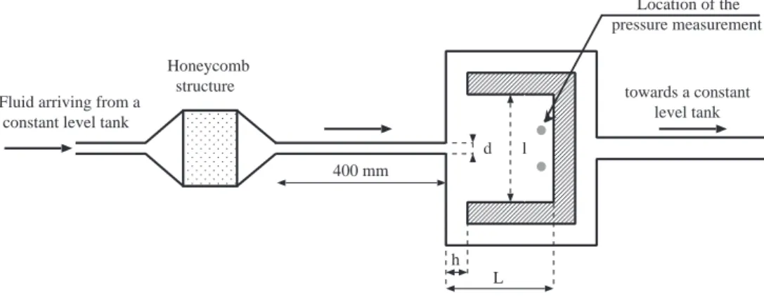
Honeycomb structure 400 mm towards a constant level tank Location of the pressure measurement
Figure 1. Experimental setup: d = 4 mm, L = 90 mm, l = 100 mm, h = 20 mm. The thickness H of the cavity is 20 mm.
The route toward high-Reynolds-number turbulence comprises successive stages related to oscillation frequency and spatial pattern modifications. In a fixed geometry (obstacle shape, impinging distance, etc), the flow oscillates with increasing frequency above the instability threshold while the Reynolds number increases. The increase is monotonic up to the first frequency discontinuity, characterized by a spatial modification of the flow pattern (modal transition). The frequency always jumps towards a higher value. This modal transition occurs with the observation of new frequencies in the temporal power spectra (peaks are clearly identified for fundamental and harmonic frequencies). Further increasing the Reynolds number leads to a similar behavior. The frequency related to the maximum amplitude in the spectra increases continuously up to a second discontinuity and so on, until the flow eventually reaches turbulence by nonlinear interactions of existing modes. Although the relation between frequency discontinuities and flow pattern transition is not yet clear, the overall behavior of impinging flows often follows this classic scenario of evolution (Rockwell and Naudasher 1979). For each frequency discontinuity, the system selects a flow pattern with a shorter wavelength, presumably based on energy budget differences and dissipation level. It is widely accepted in the literature that the onset of such a globally organized behavior in confined geometry is due to a feedback loop (Chanaud and Powell1965, Ho and Nosseir1981, Crighton1992). Inlet flow disturbances grow while being advected and interact with the impingement point. The feedback loop induces an unsteady forcing of the inlet flow, resulting in a periodic cycle. The physical nature of this feedback may be hydrodynamic or acoustic.
In this paper, we are interested in the geometric configuration of a confined jet impinging on a flat wall. In a previous study, we investigated the dynamics of the impingement of a water jet on a deformable free surface (Bouchet et al 2002). The water jet penetrated the cavity and impacted the water/air interface vertically from below. Resonant behavior set in when deformations of the free surface were dynamically coupled with large-scale meandering of the jet. The wavelength and frequency of the jet oscillation exhibited an unexpected evolution when the inlet Reynolds number was varied. We concluded that there was a strong coupling between the flexible nature of the free surface and the natural oscillation modes of the jet. In this paper, the configuration is similar to that of our previous study except that the impinged surface is a solid wall. We aim to understand the respective roles of the jet instability itself and the sloshing modes of the free surface. The geometric configuration (see figure1) is simple and can be seen as an idealized device for fluid injection into a confined chamber.
Usually, industrial applications deal with strongly turbulent flows (Varieras et al2001) but instabilities occurring at small Reynolds numbers have intrinsic dynamics comparable to large-scale coherent structures embedded in the turbulent flow. In the present study, the inlet Reynolds number is moderate (< 500) and turbulent effects are minor. The response of the flow is mainly controlled by large-scale self-sustained oscillations related to the geometric confinement.
2. Experimental setup
The experimental device was a cuboid cavity supplied with water. It was 20 mm high (denoted by H ), 90 mm long (streamwise confinement L) and 100 mm wide (spanwise confinement l). The fluid entered the cavity by a 400 mm long channel ending in a rectangular section 4 mm wide (d) and 20 mm thick. The fluid exited by two side channels of square section (20 mm side) located on each side upstream of the cavity (see figure1). Because of the small thickness of the cavity, we expected three-dimensional (3D) distortion of the flow to have negligible effect on instabilities. Spanwise modes of instability were undoubtedly damped by viscous dissipation due to the proximity of the walls. Visualizations with dyed water showed a sharp contour of the inlet jet until impingement. This confirmed that small-scale turbulence and 3D modes were absent. A honeycomb structure was inserted upstream of the cavity to reduce perturbations. We noted that, because of the long distance between the honeycomb structure and the cavity inlet, the channel flow was fully developed. Using a laser Doppler anemometer, we verified that, due to the long inlet channel, the velocity profile in the spanwise direction was perfectly parabolic. This was the case while the Reynolds number (based on the mean velocity
Uand the width of the injection channel d) was lower than 400. However, beyond Re = 400, the velocity profile was slightly flattened as observed by Wygnanski and Champagne (1973) for such square channels. The experimental configuration allowed jet velocities U lower than 0.125 m s−1(U is the mean velocity at the jet nozzle). Injection was gravity driven and water
flowed in a closed loop between constant level tanks located upstream and downstream of the device (keeping the flow rate constant). This setup prevented parasitic frequencies that could have perturbed the flow. The flow rate was regulated with a needle valve and measured by an electromagnetic flowmeter, with an accuracy of 0.4% full scale. The Reynolds number could be varied from 5 to 500 (the experimental error was lower than 1%). To characterize the behavior of flow instabilities, the velocity fluctuations in the cavity were probed by a differential pressure transducer (full scale range 56 Pa), along with a demodulator. The detection holes of the pressure transducer (high-precision variable reluctance) were located symmetrically with respect to the symmetry axis of the cavity (85 mm from the inlet, see figure1). Then, the signal of the demodulator was processed through an active low-pass filter and digitized on a computer. To measure the frequency of the oscillations, we used a sampling frequency of 10 Hz with 215 points, each measurement point corresponding to a recording
over almost 3300 s—nearly 1 h. This provided a resolution frequency of 3 × 10⁻⁴Hz.
3. Experimental results
When the Reynolds number Re =U dν was lower than 219, no oscillation was detected by the pressure sensor. Visualization by means of a dye (black Eriochrome) confirmed that, for such Reynolds numbers, the flow was steady and symmetric. The system was composed of a jet flowing along the symmetry axis of the cavity, presenting weak spreading and impacting the downstream wall of the cavity. It corresponded to the base flow obtained by
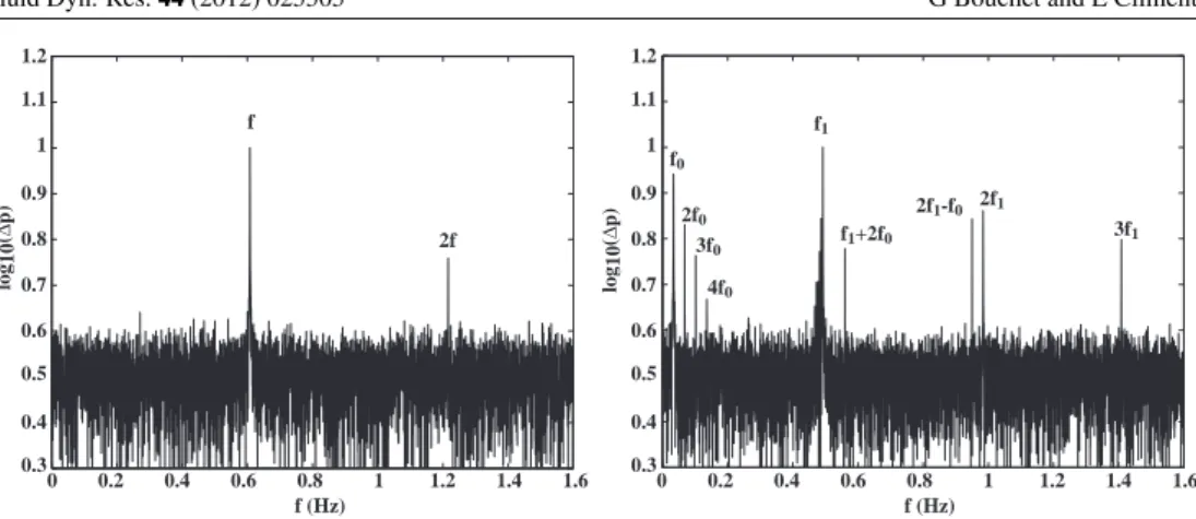
Fluid Dyn. Res. 44 (2012) 025505 G Bouchet and E Climent log 10 (Δ p) f 2f 0 0.2 0.4 0.6 0.8 1 1.2 1.4 1.6 0.3 0.4 0.5 0.6 0.7 0.8 0.9 1 1.1 1.2 0.3 0.4 0.5 0.6 0.7 0.8 0.9 1 1.1 1.2 f (Hz) 0 0.2 0.4 0.6 0.8 1 1.2 1.4 1.6 f (Hz) log 10 (Δ p) f0 f1 2f0 3f0 4f0 f1+2f0 2f1 3f1 2f1-f0
Figure 2. Power spectra of the differential pressure: (a) Re = 219 and (b) Re = 240.
0 10 20 30 40 50 60 -0.5 -0.4 -0.3 -0.2 -0.1 0 0.1 0.2 0.3 0.4 0.5 time (s)
Differential pressure (Pa)
0 0.2 0.4 0.6 0.8 1 1.2 1.4 1.6 0.3 0.4 0.5 0.6 0.7 0.8 0.9 1 1.1 1.2 f(Hz) log 10 (Δ p) f0 2f0 3f0 4f0 f1 f2 3f1-3f2 2f1 3f1 2f2 f1+2f0 f1+f2 2f1+f2
Figure 3. (a) Temporal evolution of the pressure for Re = 229 (beat between f0and f1); (b) power
spectrum for Re = 249.
the numerical simulations in the second part of our study (see figure7). The flow field was divided into two parts, revealing two symmetrical recirculations, one on either side of the jet axis. Lastly, the flow left the cavity by the two side channels. For Re = 219, the hydrodynamic system became unsteady and oscillated with a well-defined frequency f = 0.608 Hz (clearly identified on the power spectrum, figure2(a)). The visualization showed that the jet oscillated in a sinusoidal way although it was not possible to measure the wavelength of the oscillation precisely by image processing. The signal-to-noise ratio was high, so we could distinguish the presence of the first harmonic 2 f . We observed this mono-frequency behavior up to Re = 229, with a weak linear increase of the frequency f with U . Beyond Re = 229, the system became bi-periodic, associated with a limiting torus characterized by two basic frequencies
f0= 0.034 Hz and f1= 0.411 Hz. The frequency f1 dominated. Besides these two basic
frequencies, linear combinations of f0 and f1 were detected (see figure 2(b)). Depending
on the Reynolds number, the number of these combinations could vary. In figure3(a), the temporal signal of pressure is presented for Re = 229: it shows beating oscillations between the frequencies f0 and f1 (with low-amplitude noise superimposed). At Re = 249, a third
frequency f2= 0.341 Hz appears (which is not a linear combination of f0and f1). This new
0 0.1 0.2 0.3 0.4 0.5 0.6 0.7 0.8 Reynolds number f(Hz) 210 220 230 240 250 260 270 280 0 0.2 0.4 0.6 0.8 1 1.2 Reynolds number 210 220 230 240 250 260 270 280 Strouhal number f f1 f2 f0
Figure 4. (a) Frequency evolution versus Reynolds number: dominant frequencies are indicated by circles; (b) Strouhal number evolution versus Reynolds number (symbols as in (a)).
in figure3(b). We also noted that, inside each stage (219< Re < 229, 229 < Re < 249 and
Re> 249), the frequencies grew linearly with the Reynolds number, leading to constant
values of the Strouhal number St = f LU . We have brought all the experimental data together
on figure4(a) (for each Reynolds number, the dominant frequency is represented by a circle). We can see that, for the last stage, the signal-to-noise ratio decreased as the Reynolds number increased. The oscillation frequencies were undetectable beyond Re = 277. We varied the Reynolds number up to 500 without observing new features.
To summarize the experimental observations, we can say that, first of all, experiments showed that the system developed an instability which set in at a critical Reynolds number of Re = 219. The instability corresponded to a sinusoidal oscillation of the jet. The first atypical result was an apparent stability of the system beyond Re = 277. In addition, the dominant frequencies increased continuously with U . We observed discrete frequency jumps, leading to a decrease in frequency at each discontinuity (see figure4(a)). Such a behavior was unexpected for a confined jet instability. Usually, frequency jumps occur with an increase of the frequency at each modal transition (Rockwell and Naudasher1979). Using the dimensionless dominant frequency (Strouhal number St = f LU), all data can be collapsed
into a single diagram (see figure 4(b)). The nearly constant value of St indicates that the dependence f(U) is linear and that the slope is reduced at each jump. It is commonly accepted (Chanaud and Powell1965, Rockwell and Naudasher1979) that frequency discontinuities are related to modal transitions, i.e. the hydrodynamic system selecting a different oscillation frequency as the flow field pattern is modified. Theoretical evidence for such modal transitions is unavailable as yet and is probably connected to an energy budget of every possible coexisting flow. Also, it has been observed that the propagation celerity of all modes is constant around U/2 (Maurel et al 1996). Consequently, for a given mode, the frequency increases linearly with the jet velocity, as observed in our case. However, if the propagation celerity increases linearly with U whereas the Strouhal number decreases as U increases, this means that the wavelength increases with Reynolds number. Such a behavior is very unusual since the system selects a mode of oscillation with larger length scales as the velocity increases. To the best of our knowledge, this type of behavior has been observed only in the case of a submerged fountain (i.e. a jet impinging on a water/air free surface) (Bouchet
Figure 5. Definition of the characteristic lengths of the mesh.
4. Numerical simulations
To obtain more information on the spatial structure of the velocity field (pattern selection and wavelength) and on the response of the system to modifications of the geometric parameters (streamwise and spanwise confinements, width of the input and outflow channels), we performed numerical simulations over a range of Reynolds numbers from steady flow to the upper bound of the unsteady periodic regime. Based on our experimental results, all simulations were performed in a 2D domain.
We solved the equations of fluid motion for the unsteady flow of an incompressible fluid of densityρ and dynamic viscosity µ. The flow was injected into a cavity through a nozzle (see the geometry on figure5). We used the Cartesian coordinates (x, y), the x-axis being parallel to the inflow direction. Spatial coordinates and velocities were scaled by inflow parameters:
dthe width of the channel and U the injection velocity.
The velocity field was the solution of the unsteady dimensionless incompressible Navier–Stokes equations (equations (1) and (2)).
∂Ev
∂t +(Ev · E∇)Ev = − E∇ p + ν∇
2
Ev, (1)
∇ · Ev = 0, (2)
whereν = Re1 stands for the inverse of the Reynolds number.
To solve these equations, we used a numerical method based on a spectral decomposition of the equations within spatial finite elements. The x–y domain (figure 5) was broken up into K spectral elements (see Patera (1984) and Karniadakis (1990)), standard high-order Lagrangian finite elements, with a variable number, N , of the Gauss–Lobatto–Legendre collocation points in each direction within the spectral element. The discretized equations were integrated in time using a semi-implicit method.
The convergence to the exact solution using a spectral element method was achieved either by increasing the number of macro-elements, K , or by increasing the number of collocation points, N . In the first case, the error decreases algebraically like K−N, where N is
fixed. When the number of the spectral elements K is constant and the polynomial order, N , increases, the error decreases exponentially as e−δ N, whereδ is constant. The discretization
into spectral elements allowed the computational effort to be distributed in an optimal way within the domain. The final accuracy was achieved preferably by increasing the spectral element order.
Fluid Dyn. Res. 44 (2012) 025505 G Bouchet and E Climent Table 1. Critical Reynolds number for various inflow and outflow channel lengths.
Inflow channel length Outflow channel length Reynolds number
1 4 98.5 2 4 100.02 3 4 100.5 4 4 100.58 5 4 100.6 3 2 101.5 3 3 100.7 3 5 100.49 3 6 100.48
The dimensionless 2D geometry was identical to the experimental configuration presented in figure 1: a rectangular cavity (L × l), with a nozzle of width d = 1 and two outflow side channels of width h.
The boundary conditions simulated an inflow in the upstream direction of the channel entering the cavity and an outflow condition on the lateral outflow channels. A no-slip condition was applied along the cavity walls. The inflow boundary condition was a parabolic velocity profile u =32∗ (1 − (
2y
d )
2), v = 0. The outflow condition assumed that both the
pressure and the viscous stresses were zero. This outflow condition, imposed in a weak form, allowed the disturbances to leave the domain without reflection and avoided confinement effects of the lateral channels.
The spectral-element mesh discretizing the (x, y) domain was selected after a specific study of the dependence of the results on the following parameters (see figure5):
• length of the upstream inflow channel (lin),
• length of downstream outflow channels (lout),
• domain discretization into spectral elements (K ) and
• order of the polynomial interpolation (the number of collocation points per spatial direction) of the N spectral elements.
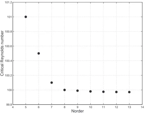
Numerical tests of the spectral-element decomposition consisted in checking that the threshold of the primary instability was independent of the mesh. We started by testing the effect of the inflow and outflow channel lengths. For these tests, we set the geometric parameters to L = 10d, l = 10d and h = 2d and the number of collocation points to N = 6 (N = 6 means a total number of 36 collocation points within each spectral element). The resulting thresholds are summarized in table 1. The following step consisted in splitting the domain into spectral elements. Lastly, we tested the effect of N order (the number of collocation points). The results are presented in figure6.
All these tests allowed us to select the optimal domain: lin= 3, lout= 4 and N = 8. The
final mesh contained about 2 × 10⁴nodes.
Before investigating the influence of the various geometric parameters, the reference case corresponded to L = 10, l = 10, h = 2 and d = 1. The simulations showed that, for
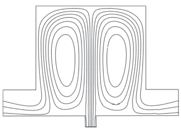
Re< 100, the flow was steady and symmetric. The streamlines of the base flow are
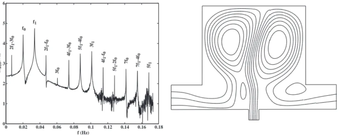
represented in figure7. Beyond Re = 100, a sinusoidal oscillation of the flow occurs. Then, the power spectrum of the velocity reveals two oscillation frequencies f0= 0.02 and f1=
0.0335, together with linear combinations of f0 and f1 (see figure8(a)); the wavelength is
approximately 1.3L (actually the wavenumber is not constant on the jet axis, and we give only an average value). Figure8(b) presents the streamlines of the disturbed flow. When the
0 0.02 0.04 0.06 0.08 0.1 0.12 0.14 0.16 0.18 0 1 2 3 4 5 6 f (Hz) log 10 (Vx) f0 f1 2f1 -3f 0 5f1 2f1 -f0 3f0 4f1 -3f 0 5f1 -4f 0 3f1 4f1 -f0 5f1 -2f 0 7f0 7f1 -4f 0
Figure 6. Convergence of the critical Reynolds number with the number of collocation points.
Re 91 100 118 0 1000 2000 3000 4000 5000 6000 7000 -0.5 -0.4 -0.3 -0.2 -0.1 0 0.1 0.2 0.3 0.4 0.5 time Spanwise velocity
V
Figure 7. Streamlines of the base flow for Re = 95 (numerical simulations).
Reynolds number increases, the frequencies f0and f1increase while the spectrum becomes
broadband. Lastly, with Re = 118, we observe a collapse of the oscillations, the amplitude of the temporal velocity signal decaying to a quasi-steady state (the amplitude is 100 times weaker: see figure9(a)). In addition, if the Reynolds number is decreased from the disturbed flow towards Re = 100, we note that the oscillation is maintained for Reynolds numbers lower than the critical value: the frequencies f0 and f1 decrease with Re. Below Re = 95,
the amplitude associated with frequency f0vanishes (only f1 appears on the spectrum, with
several harmonics). Lastly, at Re = 91, the oscillation stops; the system recovers its base flow. Finally, we tried to disturb the base flow for a Reynolds number ranging from 91 to 100. Depending on the initial amplitude of the disturbance, we found that the system could either damp or amplify the disturbance to bifurcate towards the oscillating solution found previously (starting at Re> 100). Consequently, we highlighted a jet instability presenting a subcritical bifurcation and disappearing beyond Re = 118 (see figure 9(b)). Thus, we varied all the geometric parameters. Varying the height of the outflow channels (changing h = 2 to h = 1) did not induce any noticeable modification of the thresholds and the oscillation frequencies. The confinement length was gradually varied from L = 9 to L = 12. Both the thresholds and the frequencies of oscillation were sensitive to this parameter. Concerning the thresholds, we noted that they decreased when L increased, which tends to show that L has a destabilizing effect. This is a common result for confined jets (Rockwell and Naudasher1979). In addition,
L lout l d h in l
Figure 8. (a) Power spectrum of the spanwise velocity on the centerline of the cavity (Re = 100); (b) streamlines of the oscillating flow (Re = 100).
4 5 6 7 8 9 10 11 12 13 14 99.8 100 100.2 100.4 100.6 100.8 101 101.2 Norder
Critical Reynolds number
Figure 9. (a) Collapse of oscillations for Re = 118; (b) stability diagram for the configuration (L = 10; l = 10; d = 1; h = 2): V represents the maximum spanwise velocity in the middle of the cavity, on the axis.
the gap between the lower threshold and the higher threshold of the subcritical bifurcation tended to decrease when L increased. The gap between the lowest and highest threshold Reynolds numbers was only 0.5 when L = 12. Scaling the frequencies by the streamwise confinement and the inlet velocity (i.e. the Strouhal number), all the data collapsed on to a single curve. Therefore, the relevant parameters for describing the instability are the Reynolds
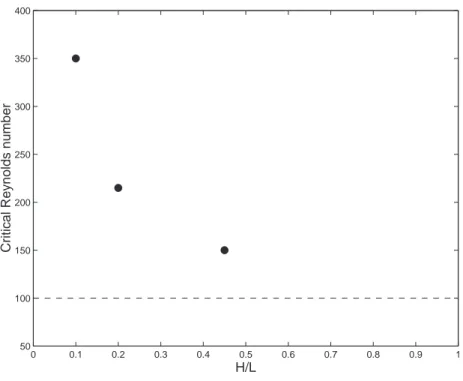
0 0.1 0.2 0.3 0.4 0.5 0.6 0.7 0.8 0.9 1 50 100 150 200 250 300 350 400 H/L
Critical Reynolds number
Figure 10. Effect of cavity thickness on the critical Reynolds number. Dashed line: threshold based on numerical simulations of 2D flow.
and Strouhal numbers. Note that for L> 12, we observed that a steady instability developed: the jet began to stick to one of the two sidewalls of the cavity according to the Coanda effect (Shapira et al1990). The selection of the sticking wall was random and depended only on the distribution of the numerical noise.
5. Conclusion and discussion
The numerical simulations showed a very similar behavior to those obtained in the experimental study. In both cases, we found that the jet instability appeared for moderate Reynolds numbers, and collapsed approximately 25% above the threshold. In both cases above the threshold, spectra contained a single characteristic frequency and its harmonics (characteristic of a limit cycle). When Re was increased further, these spectra showed two frequencies and linear combinations of these two frequencies (which is characteristic of a limiting torus). However, the numerical thresholds (approximately 100) were much lower than the experimental thresholds (close to 200). This quantitative disagreement is certainly related to 3D effects in the experimental cavity. To draw this conclusion, we performed an experimental study on a cavity with a variable thickness in order to determine the effect of the aspect ratio H/L (where H is the thickness of the cavity and L the streamwise confinement) on the threshold of the instability. Thus we used two new cavities, geometrically similar to the first one but with thicknesses H = 40 mm (H/L = 0.44) and H = 10 mm (H/L = 0.11). We represent the evolution of the critical Reynolds number for various aspect ratios H/L in figure10. The figure shows that the instability threshold decreases when the thickness of the cavity increases. This type of evolution has already been observed in other configurations (see, for example, wake instability Mathis et al (1984)). It was shown that the threshold of
instability was a decreasing function of the ratio between the width of the cylinder and its diameter. In our case, the evolution of the threshold of instability with the ratio H/L can be explained in the following way: when the thickness of the cavity is small, the influence of the walls, through the development of boundary layers, has a stabilizing effect on the flow. It is clear that the instability threshold will be higher when the thickness of the cavity is reduced. Figure10(dashed line) represents the value of the threshold obtained numerically. If we consider that the numerical cavity is purely two dimensional, this is equivalent to the thickness of the cavity being infinite (with a negligible effect of the viscous boundary layers). Then we find good agreement between the numerical and the experimental results. Although the thresholds and Strouhal numbers found are underestimated, we can conclude that the 2D numerical study is relevant and that the instability is actually a 2D instability. The numerical study clearly shows that the Hopf bifurcation is subcritical. The height of the output channels h has no influence, but the streamwise confinement has a significant effect on the frequency selection (interpreted as a constant Strouhal number) and on the thresholds (destabilizing effect). On the other hand, we did not obtain, numerically, a modal transition associated with a frequency jump. Therefore, it is impossible to clearly state that frequency jumps observed experimentally are related to the wavelength modification of the oscillation pattern.
Acknowledgment
The authors gratefully acknowledge Claude Veit for his technical collaboration in the design and building of the experimental device.
References
Bouchet G, Climent E and Maurel A 2002 Europhys. Lett.59 827–33 Chanaud R and Powell A 1965 J. Acoust. Soc. Am.37 902–12 Crighton D 1992 J. Fluid Mech.234 361–91
Ho C and Nosseir N 1981 J. Fluid Mech.105 119–42
Karniadakis G 1990 Comput. Methods Appl. Mech. Eng.80 367–80 Mathis C, Provansal M and Boyer L 1984 J. Phys. Lett.45 483–91 Maurel A, Ern P, Zielinska B and Weisfreid J 1996 Phys. Rev. E54 3643–51 Patera A 1984 J. Comput. Phys.54 468–88
Rockwell D and Naudasher E 1979 Annu. Rev. Fluid Mech.11 67–94 Sato H 1959 J. Fluid Mech.7 53–68
Shapira M, Degani D and Weihs D 1990 Comput. Fluids18 239–58 Sondhauss C 1854 Ann. Phys., Lpz. 91 214–40
Varieras D, Gervais P, Giovannini A and Breton J 2001 Congr`es fran¸cais de thermique, SFT (Lyon, France, 15–17 May 2000)pp 235–40