Pépite | Caractérisation des canaux massive MIMO et stratégies de sélection d'antenne : application pour la 5G et l'industrie 4.0
192
0
0
Texte intégral
(2) Thèse de Frédéric Challita, Université de Lille, 2019. © 2019 Tous droits réservés.. lilliad.univ-lille.fr.
(3) Thèse de Frédéric Challita, Université de Lille, 2019. Abstract. O. ver the past decade, mobile connectivity and wireless systems have become a necessity for many applications and use-cases. Faster, smarter, safer and environment-friendlier networks are sought. Continuous efforts have been made to boost wireless systems performance, from analog to digital systems, bulky handheld cellular phone and user equipments to ever-small sensors and smart phones, from mechanization and basic automation systems to the smart industry of the future or Industry 4.0. However, current wireless networks are not yet able to fulfill the many gaps from 4G and address the requirements of 5G, or the fifth generation of mobile networks. Thus, significant technological breakthroughs are still required to strengthen wireless networks. For instance, in order to provide higher data rates and accommodate many types of equipment, more spectrum resources are needed and the currently used spectrum requires to be efficiently utilized. 5G is initially being labeled as an evolution, made available through improvements in LTE (Long-Term Evolution), but it will not be long before it becomes a revolution and a major step-up from previous generations. Massive MIMO (Multiple-Input Multiple-Output) has emerged as one of the most promising physical-layer technologies for future 5G wireless systems. The main idea is to equip base stations with large arrays (100 antennas or more) to simultaneously communicate with many terminals or user equipments. Using smart pre-processing at the array, massive MIMO promises to deliver superior system improvement with improved spectral efficiency, achieved by spatial multiplexing and better energy efficiency, exploiting array gain and reducing the radiated power. Massive MIMO can fill the gap for many requirements in 5G use-cases notably industrial IoT (Internet of Things) in terms of data rates, spectral and energy efficiency, reliable communication, optimal beamforming, linear processing schemes and so on. Over the last 6 years, several scientific papers proved the theoretical aspects and promises of massive MIMO systems and many trials validated that this technology is not just an academic concept. However, the hardware and software complexity arising from the sheer number of radio frequency chains is a bottleneck and some challenges are still to be tackled before the full operational deployment of massive MIMO. For instance, reliable channel models, impact of polarization diversity, 3. © 2019 Tous droits réservés.. lilliad.univ-lille.fr.
(4) Thèse de Frédéric Challita, Université de Lille, 2019. optimal antenna selection strategies, mutual coupling and channel state information acquisition amongst other aspects, are all important questions worth exploring. Also, a good understanding of industrial channels is needed to bring the smart industry of the future ever closer. In this thesis, we try to address some of these questions based on radio channel data from a measurement campaign in an industrial scenario using a massive MIMO setup. The thesis main objectives are threefold: 1. Characterization of massive MIMO channels in Industry 4.0 (industrial IoT) with a focus on spatial correlation, classification and impact of cross-polarization at transmission side. The setup consists in multiple distributed user equipments in many propagation conditions. This study is based on propagationbased metrics such as Ricean factor, correlation, etc. and system-oriented metrics such as sum-rate capacity with linear precoding and power allocation strategies. Moreover, polarization diversity schemes are proposed and were shown to achieve very promising results with simple allocation strategies. This work provides comprehensive insights on radio channels in Industry 4.0 capable of filling the gap in channel models and efficient strategies to optimize massive MIMO setups are proposed. 2. Proposition of antenna selection strategies using the receiver spatial correlation, a propagation metric, as a figure of merit. The goal is to reduce the number of radio frequency chain and thus the system complexity by selecting a set of distributed antennas. The proposed strategy achieves near-optimal sum-rate capacity with less radio frequency chains. This is critical for massive MIMO systems if complexity and cost are to be reduced. 3. Proposition of an efficient strategy for overhead reduction in channel state information acquisition of FDD (frequency-division-duplex) systems. The strategy relies on spatial correlation at the transmitter and consists in solving a set of simple autoregressive equations (Yule-Walker equations). The results show that the proposed strategy achieves a large fraction of the performance of TDD (time-division-duplex) systems initially proposed for massive MIMO.. 4. © 2019 Tous droits réservés.. lilliad.univ-lille.fr.
(5) Thèse de Frédéric Challita, Université de Lille, 2019. Résumé. D. ans le domaine des télécommunications sans fil, des efforts importants se sont portés ces dix dernières années sur le développement de systèmes d’échange d’information rapides, intelligents, sûrs et respectueux de l’environnement. Les domaines applicatifs sont de plus en plus larges, s’étendant par exemple du grand public, à la voiture connectée, à l’internet des objets (IoT Internet of Things) et à l’industrie 4.0. Dans ce dernier cas, l’objectif est d’aboutir à une flexibilité et à une versatilité accrues des chaînes de production et à une maintenance prédictive des machines, pour ne citer que quelques exemples. Cependant, les réseaux sans fil actuels ne sont pas encore en mesure de répondre aux nombreuses lacunes de la quatrième génération des réseaux mobiles (4G) et aux exigences de la 5G quant à une connectivité massive, une ultra fiabilité et des temps de latence extrêmement faibles. L’optimisation des ressources spectrales est également un point très important. La 5G était initialement considérée comme une évolution, rendue possible grâce aux améliorations apportées à la LTE (Long-Term Evolution), mais elle ne tardera pas à devenir une révolution et une avancée majeure par rapport aux générations précédentes. Dans ce cadre, la technologie des réseaux massifs ou Massive MIMO (Multiple-Input Multiple-Output) s’est imposée comme l’une des technologies de couche physique les plus prometteuses. L’idée principale est d’équiper les stations de base de grands réseaux d’antennes (100 ou plus) pour communiquer simultanément avec de nombreux terminaux ou équipements d’utilisateurs. Grâce à un prétraitement intelligent au niveau des signaux d’émission, les systèmes massive MIMO promettent d’apporter une grande amélioration des performances, tout en assurant une excellente efficacité spectrale et énergétique. De nombreux articles scientifiques ont développé récemment les aspects théoriques de ces systèmes dont la faisabilité a été validée par des essais réalisés par des opérateurs. Cependant, certains défis doivent encore être relevés avant le déploiement complet des communications basées sur le massive MIMO. Par exemple, l’élaboration de modèles de canaux représentatifs de l’environnement réel, l’impact de la diversité de polarisation, les stratégies de sélection optimale d’antennes et l’acquisition d’informations d’état du canal, sont des sujets importants à explorer. En outre, une bonne compréhension des canaux de propagation en milieu industriel est nécessaire pour optimiser les 5. © 2019 Tous droits réservés.. lilliad.univ-lille.fr.
(6) Thèse de Frédéric Challita, Université de Lille, 2019. liens de communication de l’industrie intelligente du futur. Dans cette thèse, nous essayons de répondre à certaines de ces questions en nous concentrant sur trois axes principaux: 1. La caractérisation polarimétrique des canaux massive MIMO en environnement industriel. Pour cela, on étudie des scénarios correspondant à des canaux ayant ou non une visibilité directe entre émetteur et récepteur (Line-of-Sight – LOS) ou Non-LOS, et en présence de divers types d’obstacles. Les métriques associées sont soit celles utilisées en propagation telles que le facteur de Rice et la corrélation spatiale, soit orientées système comme la capacité totale du canal incluant des stratégies de précodage linéaire. De plus, les schémas de diversité de polarisation proposés montrent des résultats très prometteurs. 2. En massive MIMO, un objectif important est de réduire le nombre de chaînes de fréquences radio et donc la complexité du système, en sélectionnant un ensemble d’antennes distribuées. Cette stratégie de sélection utilisant la corrélation spatiale du récepteur, une métrique de propagation, comme facteur de mérite, permet d’obtenir une capacité totale quasi-optimale. 3. Une technique efficace de réduction des ressources temps-fréquence lors de l’acquisition d’informations du canal de propagation dans les systèmes FDD (frequency-division-duplex) est enfin proposée. Elle repose sur la corrélation spatiale au niveau de l’émetteur et consiste à résoudre un ensemble d’équations auto-régressives simples. Les résultats montrent que cette technique permet d’atteindre des performances qui ne sont pas trop éloignées de celles des systèmes TDD (time-division-duplex) initialement proposés pour le massive MIMO.. 6. © 2019 Tous droits réservés.. lilliad.univ-lille.fr.
(7) Thèse de Frédéric Challita, Université de Lille, 2019. Acknowledgements. F. irst of all, I would like to thank Mrs. Martine LIENARD, my thesis director, for accepting to guide me through these three years of thesis. Her patience, support, kindness and knowledge were most helpful during my thesis. I would like to thank her for her relevant remarks and support in writing this manuscript. I also learned a lot about gardening by listening to her passionately talk about the best ways to grow vegetables and fruits. Also, thanks for Mr. Lionel BUCHAILLOT, director of the IEMN laboratory and all the members of the IEMN for all the help during these 3 years. To my co-director Mr. Davy Gaillot, I am grateful and honored to have worked beside you. Lots of good moments were shared in these 3 years especially during conferences and presentations. I will never forget these times and I will never forget your patience, notes and help during the writing of this thesis and the different articles. I think it is important (I know you don’t like this word), to express my sincere appreciation to you on both the professional and personal aspect. Besides my advisor, I would like to thank the different members of my thesis committee, Mr. Jean-François Diouris, professor at Ecole Polytechnique de l’Université de Nantes, Mr. Pascal Pagani, research engineer HDR at CEA-CESTA, Mr. Alain Sibille , professor at TELECOM ParisTech and Mrs. Dinh-Thuy PHAN-HUY, research engineer at Orange Labs. Thank you for examining my work and for your insightful remarks that helped improve the quality of this manuscript. I am also very greatful to Mr. Joseph Wout and Mr. José-Maria Molina GarciaPardo, invited members with whom we cooperated on many subjects and research areas. Thank you both for your comments and help during these 3 years. I would also like to thank M. Degauque Pierre for his help, remarks and patience while processing measurement data for all the projects we worked on. His expertise and great mind were inspiring to me and helped me understand many concepts, especially in tunnel environments and wave propagation. To Mr. Pierre Laly, it has been a great honor to work with you on the great MIMOSA. It helped me understand electronic systems and appreciate the complexity of channel sounders. Also, I will never forget the different measurement campaigns we did together, le Havre, Gant, Anvers. Thank you for the good times we shared 7. © 2019 Tous droits réservés.. lilliad.univ-lille.fr.
(8) Thèse de Frédéric Challita, Université de Lille, 2019. together, thank you for teaching me lots and lots of things and thank you for your support. I would also like to thank Mrs. Dégardin Virginie for welcoming me in the electronic department of University of Lille and for her trust, kindness and great spirit. Thank you Mr. Eric Simon for all the good discussions we had about NOMA and research aspects of my thesis. I appreciated these good times amongst others. Last but not least, I would like to thank all my friends and colleagues who encouraged me and shared with me the good and the bad times: Ali, Navish, Grecia, Rose, Mauro, Gauthier, Shiqi, Mohammed C., Nicolas, Mahmoud, Elias, Rachel. I cannot mention them all, but I express my gratitude to you for making my stay in Lille a great one. A special thanks to my family and Lamya for always being here when I needed you. Finally, thanks again to all the people I mentioned above and to the people whom I couldn’t mention but helped me directly or indirectly during my study. Without you, I could not have achieved this success.. 8. © 2019 Tous droits réservés.. lilliad.univ-lille.fr.
(9) Thèse de Frédéric Challita, Université de Lille, 2019. Contents. List of figures. 14. List of tables. 18. List of publications. 20. 1 General Introduction and Motivations 1.1 Introduction: Overview of The 5th Generation . . . . . 1.1.1 5G: Evolution or Revolution ? . . . . . . . . . . 1.1.2 Initial Vision: Use-cases for 5G New Radio . . . 1.1.2.1 Use-Cases . . . . . . . . . . . . . . . . 1.1.2.2 Multi-Layer Spectrum . . . . . . . . . 1.1.3 Gaps and Challenges . . . . . . . . . . . . . . . 1.2 Impacting technologies of 5G . . . . . . . . . . . . . . 1.2.1 Massive MIMO: Why Now ? . . . . . . . . . . . 1.3 Multi-antenna System Communications . . . . . . . . . 1.3.1 MIMO Communications . . . . . . . . . . . . . 1.3.1.1 Fundamentals and system model . . . 1.3.2 Multi-User MIMO . . . . . . . . . . . . . . . . 1.3.2.1 Advantages of MU-MIMO . . . . . . . 1.3.3 Evolution of multi-antenna systems with 3GPP 1.4 Massive MIMO: Massive Breakthrough . . . . . . . . . 1.4.1 History and Brief Introduction . . . . . . . . . . 1.4.2 General Definitions . . . . . . . . . . . . . . . . 1.4.3 Key Features . . . . . . . . . . . . . . . . . . . 1.4.4 Main Advantages . . . . . . . . . . . . . . . . . 1.5 Massive MIMO System Architecture . . . . . . . . . . 1.5.1 Digital Beamforming (DBF) . . . . . . . . . . . 1.5.2 Analog Beamforming (ABF) . . . . . . . . . . . 1.5.3 No Compromise ? . . . . . . . . . . . . . . . . . 1.5.4 What is precoding then ? . . . . . . . . . . . .. 25 25 25 26 26 27 29 30 31 32 32 32 33 34 35 36 36 39 40 40 43 43 43 43 45. . . . . . . . . . . . . . . . . . . . . . . . .. . . . . . . . . . . . . . . . . . . . . . . . .. . . . . . . . . . . . . . . . . . . . . . . . .. . . . . . . . . . . . . . . . . . . . . . . . .. . . . . . . . . . . . . . . . . . . . . . . . .. . . . . . . . . . . . . . . . . . . . . . . . .. . . . . . . . . . . . . . . . . . . . . . . . .. . . . . . . . . . . . . . . . . . . . . . . . .. 9. © 2019 Tous droits réservés.. lilliad.univ-lille.fr.
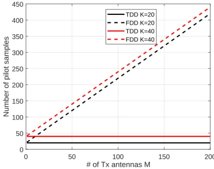
(10) Thèse de Frédéric Challita, Université de Lille, 2019. Contents. 1.6. Massive MIMO in practice . . . . . . . . . . . . . . . . . . . . . . . 1.6.1 Real-time Testbeds . . . . . . . . . . . . . . . . . . . . . . . 1.6.2 Trials and Deployments . . . . . . . . . . . . . . . . . . . . 1.6.3 Challenges . . . . . . . . . . . . . . . . . . . . . . . . . . . . 1.7 Channel Estimation . . . . . . . . . . . . . . . . . . . . . . . . . . . 1.7.1 Time Division Duplexing . . . . . . . . . . . . . . . . . . . . 1.7.2 Frequency Division Duplexing . . . . . . . . . . . . . . . . . 1.7.2.1 Coherence Interval . . . . . . . . . . . . . . . . . . 1.7.2.2 5G Frame Structure . . . . . . . . . . . . . . . . . 1.8 Motivations and Contributions . . . . . . . . . . . . . . . . . . . . . 1.8.1 Special Focus on Industry 4.0 . . . . . . . . . . . . . . . . . 1.8.2 Polarimetric Channel Characteristics and Propagation Conditions . . . . . . . . . . . . . . . . . . . . . . . . . . . . . . . 1.8.3 CSI Feedback Overhead Reduction . . . . . . . . . . . . . . 1.8.4 Antenna Selection Strategies . . . . . . . . . . . . . . . . . . 1.9 Thesis Organization . . . . . . . . . . . . . . . . . . . . . . . . . . . 1.10 Other Contributions . . . . . . . . . . . . . . . . . . . . . . . . . . 1.11 Summary of Key Points . . . . . . . . . . . . . . . . . . . . . . . . 2 Massive MIMO Channel and System Aspects 2.1 SISO Wireless Propagation Channel . . . . . . . . . . . 2.1.1 Characteristics of Propagation Channels . . . . 2.1.1.1 Large scale propagation . . . . . . . . 2.1.1.2 Small scale propagation . . . . . . . . 2.1.2 Time-Frequency Domain SISO Channel Model . 2.1.2.1 Delay Domain Analysis . . . . . . . . 2.1.2.2 Frequency domain analysis . . . . . . 2.2 Massive MIMO Channel Characteristics . . . . . . . . 2.2.1 Notations . . . . . . . . . . . . . . . . . . . . . 2.2.2 General Propagation Parameters . . . . . . . . 2.2.2.1 Average Channel Gain . . . . . . . . . 2.2.2.2 Cross-Polarization Discrimination . . . 2.2.2.3 Ricean Factor . . . . . . . . . . . . . . 2.2.2.4 Spatial Correlation . . . . . . . . . . . 2.2.3 The Two Characteristics of Massive MIMO . . . 2.2.3.1 Channel Hardening . . . . . . . . . . . 2.2.3.2 Favorable Propagation Condition . . . 2.2.4 The Gram Matrix . . . . . . . . . . . . . . . . . 2.2.4.1 Gram’s matrix Power Ratio . . . . . . 2.3 Massive MIMO Channel Model . . . . . . . . . . . . . 2.3.1 Review of Correlation-based Channel Models . . 2.3.2 Geometrical based Propagation Channel Model 2.3.2.1 Special Case: Rayleigh Channel Model. . . . . . . . . . . . . . . . . . . . . . .. . . . . . . . . . . . . . . . . . . . . . . .. . . . . . . . . . . . . . . . . . . . . . . .. . . . . . . . . . . . . . . . . . . . . . . .. . . . . . . . . . . . . . . . . . . . . . . .. . . . . . . . . . . . . . . . . . . . . . . .. . . . . . . . . . . . . . . . . . . . . . . .. . . . . . . . . . . .. 46 46 46 47 48 48 49 49 49 51 51. . . . . . .. 51 52 52 52 53 55. . . . . . . . . . . . . . . . . . . . . . . .. 57 58 58 58 59 60 60 61 61 61 63 63 64 64 65 67 68 69 69 69 70 71 71 73. 10. © 2019 Tous droits réservés.. lilliad.univ-lille.fr.
(11) Thèse de Frédéric Challita, Université de Lille, 2019. Contents. 2.4. 2.5. 2.6 2.7. 2.3.2.2 Improving Stochastic Models . . . . . . 2.3.3 Parametric Analysis . . . . . . . . . . . . . . . . 2.3.3.1 Channel Hardening . . . . . . . . . . . . 2.3.3.2 Gram’s Power Ratio . . . . . . . . . . . System Model for DL Massive MIMO . . . . . . . . . . . 2.4.1 System performance: Capacity of MIMO systems 2.4.1.1 Capacity of SU-MIMO . . . . . . . . . 2.4.2 Capacity of MU-MIMO . . . . . . . . . . . . . . 2.4.2.1 Power Allocation . . . . . . . . . . . . . 2.4.2.2 Precoding Strategies . . . . . . . . . . . 2.4.2.3 Maximum-Ratio-Transmission . . . . . . 2.4.2.4 Zero-Forcing . . . . . . . . . . . . . . . 2.4.2.5 Minimum Mean-Squared Error . . . . . 2.4.3 Performance Analysis: Simplified System Model . 2.4.3.1 Massive MIMO and Linear Processing . Sum-Rate Capacity Results . . . . . . . . . . . . . . . . 2.5.1 Performance in i.i.d. Channels . . . . . . . . . . . 2.5.2 Parametric Analysis with the Geometrical Model Conclusion . . . . . . . . . . . . . . . . . . . . . . . . . . Summary of Key Points . . . . . . . . . . . . . . . . . .. . . . . . . . . . . . . . . . . . . . .. . . . . . . . . . . . . . . . . . . . .. . . . . . . . . . . . . . . . . . . . .. 3 Polarimetric Massive MIMO Channel Measurements in an try 4.0 3.1 Introduction: Industry 4.0 . . . . . . . . . . . . . . . . . . . . 3.2 Review of Massive MIMO Channel Characterization . . . . . . 3.2.1 Sounding Techniques . . . . . . . . . . . . . . . . . . . 3.2.2 Review of Main Results . . . . . . . . . . . . . . . . . 3.3 Experimental Setup . . . . . . . . . . . . . . . . . . . . . . . . 3.3.1 Radio Channel Sounding . . . . . . . . . . . . . . . . . 3.3.2 Antennas . . . . . . . . . . . . . . . . . . . . . . . . . 3.4 Geometrical Configuration of the Experiments . . . . . . . . . 3.4.1 Multi-User Setup . . . . . . . . . . . . . . . . . . . . . 3.4.2 General Notations . . . . . . . . . . . . . . . . . . . . 3.4.2.1 Polarimetric Massive MIMO Channel Matrix 3.5 Propagation Channel Characteristics . . . . . . . . . . . . . . 3.5.1 Channel Transfer Function: Example . . . . . . . . . . 3.5.2 Average Received Gain . . . . . . . . . . . . . . . . . . 3.5.3 Coherence BW, Ricean factor and Tx Correlation . . . 3.5.4 Classification . . . . . . . . . . . . . . . . . . . . . . . 3.5.5 Selected Scenarios . . . . . . . . . . . . . . . . . . . . . 3.5.6 Parameter Cross-Correlation . . . . . . . . . . . . . . . 3.5.7 Polarimetric Channel Characteristics . . . . . . . . . . 3.6 Massive MIMO System Evaluation . . . . . . . . . . . . . . .. . . . . . . . . . . . . . . . . . . . .. . . . . . . . . . . . . . . . . . . . .. . . . . . . . . . . . . . . . . . . . .. . . . . . . . . . . . . . . . . . . . .. 73 74 74 75 76 77 78 78 79 80 81 81 82 82 83 83 83 85 88 88. Indus. . . . . . . . . . . . . . . . . . . .. . . . . . . . . . . . . . . . . . . . .. . . . . . . . . . . . . . . . . . . . .. . . . . . . . . . . . . . . . . . . . .. 89 89 90 91 91 93 93 94 96 96 96 96 99 99 99 100 102 104 104 105 106. 11. © 2019 Tous droits réservés.. lilliad.univ-lille.fr.
(12) Thèse de Frédéric Challita, Université de Lille, 2019. Contents. 3.6.1 3.6.2 3.6.3. 3.7. 3.8 3.9. Does Channel Hardening hold ? . . . . . . . . How Favorable is the Propagation ? . . . . . . Gram’s Power Ratio . . . . . . . . . . . . . . 3.6.3.1 Influence of the Scenario . . . . . . . 3.6.4 Sum-rate Capacity: . . . . . . . . . . . . . . Communication Strategy Using Polarization Diversity 3.7.1 UEs Allocation Algorithms . . . . . . . . . . . 3.7.2 Results . . . . . . . . . . . . . . . . . . . . . . Conclusion . . . . . . . . . . . . . . . . . . . . . . . . Summary of Key Points . . . . . . . . . . . . . . . .. . . . . . . . . . .. . . . . . . . . . .. . . . . . . . . . .. . . . . . . . . . .. . . . . . . . . . .. . . . . . . . . . .. 4 Propagation-Based Antenna Selection Strategies 4.1 CSI Feedback Reduction in FDD mode . . . . . . . . . . . . . . 4.1.1 Context and Methodologies . . . . . . . . . . . . . . . . 4.1.1.1 Related Work . . . . . . . . . . . . . . . . . . . 4.1.1.2 Preview of the Method . . . . . . . . . . . . . . 4.1.1.3 Framework For Channel Estimation . . . . . . 4.1.2 Estimation Procedure . . . . . . . . . . . . . . . . . . . 4.1.2.1 Tx Correlation . . . . . . . . . . . . . . . . . . 4.1.2.2 Principle of CSIT Estimation Procedure . . . . 4.1.2.3 Determination of the reduced correlation vector 4.1.2.4 Estimation of the channel matrix . . . . . . . . 4.1.3 Optimization of the Algorithm and Performances . . . . 4.1.3.1 Single-User Configuration . . . . . . . . . . . . 4.1.3.2 Multi-User Configuration . . . . . . . . . . . . 4.1.3.3 Quantifying Complexity Reduction . . . . . . . 4.1.4 Conclusion . . . . . . . . . . . . . . . . . . . . . . . . . . 4.2 Antenna Selection Strategies . . . . . . . . . . . . . . . . . . . 4.2.1 Context and Methodologies . . . . . . . . . . . . . . . . 4.2.1.1 Related Work . . . . . . . . . . . . . . . . . . . 4.2.1.2 Antenna selection Procedure . . . . . . . . . . . 4.2.1.3 Selection criterion . . . . . . . . . . . . . . . . 4.2.1.4 Evaluation Algorithm . . . . . . . . . . . . . . 4.2.1.5 Investigated Scenario . . . . . . . . . . . . . . . 4.2.2 Validation and Results . . . . . . . . . . . . . . . . . . . 4.2.2.1 Validation based on Rx correlation . . . . . . . 4.2.2.2 Strategy Performance Evaluation and Results . 4.2.2.3 Gram’s Power Ratio . . . . . . . . . . . . . . . 4.2.2.4 Parametric Analysis . . . . . . . . . . . . . . . 4.2.2.5 Sum-rate Capacity . . . . . . . . . . . . . . . . 4.2.3 Conclusion . . . . . . . . . . . . . . . . . . . . . . . . . . 4.3 General Conclusion . . . . . . . . . . . . . . . . . . . . . . . . . 5 Conclusion. . . . . . . . . . .. . . . . . . . . . . . . . . . . . . . . . . . . . . . . . .. . . . . . . . . . .. . . . . . . . . . .. 107 109 111 111 114 117 117 119 121 122. . . . . . . . . . . . . . . . . . . . . . . . . . . . . . .. 123 . 124 . 124 . 124 . 125 . 125 . 126 . 126 . 129 . 129 . 130 . 131 . 131 . 133 . 134 . 135 . 136 . 136 . 136 . 138 . 138 . 139 . 139 . 139 . 139 . 141 . 141 . 143 . 144 . 146 . 147 149. 12. © 2019 Tous droits réservés.. lilliad.univ-lille.fr.
(13) Thèse de Frédéric Challita, Université de Lille, 2019. Contents. 6 Future Research Directions. 153. Appendix. 156. A List of Notations, Symbols and Acronyms A.0.1 Mathematical Notations and Operators . . . . . . . . . . . . A.0.2 List of Specific Used Symbols . . . . . . . . . . . . . . . . . A.0.3 List of Acronyms . . . . . . . . . . . . . . . . . . . . . . . .. 157 . 157 . 158 . 160. B DPC and Waterfilling 163 B.1 Dirty Paper Coding . . . . . . . . . . . . . . . . . . . . . . . . . . . . 163 B.2 Waterfilling algorithm . . . . . . . . . . . . . . . . . . . . . . . . . . 163 C Ricean Factor Estimation. 165. D Geometrical Model: Charts and Validation. 167. E Antennas Characteristics. 171. F UE Allocation Strategies. 175. Bibliography. 176. 13. © 2019 Tous droits réservés.. lilliad.univ-lille.fr.
(14) Thèse de Frédéric Challita, Université de Lille, 2019. © 2019 Tous droits réservés.. lilliad.univ-lille.fr.
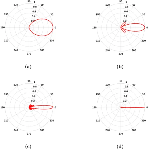
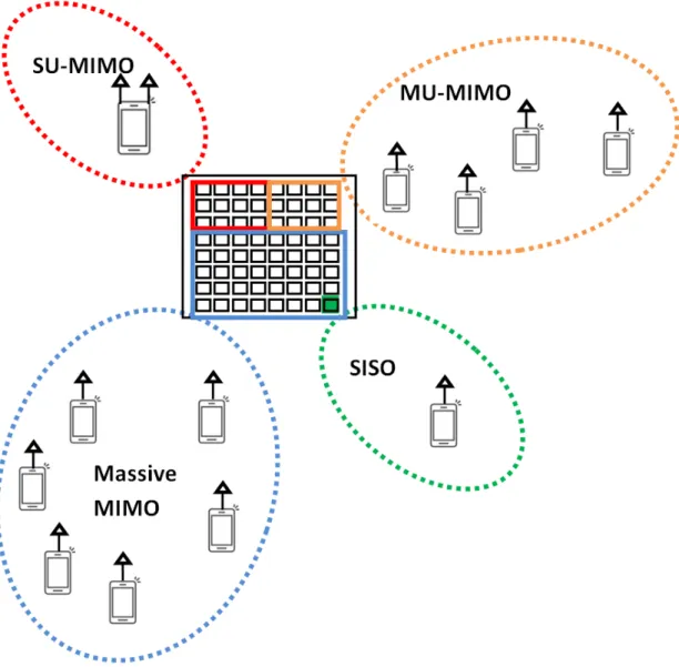
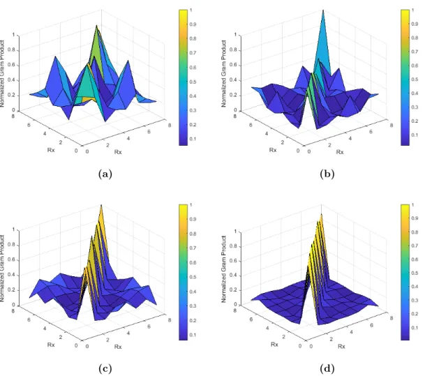
(15) Thèse de Frédéric Challita, Université de Lille, 2019. List of Figures. 1.1 1.2 1.3 1.4 1.5 1.6 1.7 1.8 1.9 1.10 1.11 1.12. 1.13 2.1 2.2 2.3 2.4 2.5 2.6 2.7. SU-MIMO system model. . . . . . . . . . . . . . . . . . . . . . . . . MU-MIMO scenario. . . . . . . . . . . . . . . . . . . . . . . . . . . 3GPP Releases-From MIMO to massive MIMO. This figure displays the evolution from Release 8 to the up-coming Release 16. . . . . . Overall Massive MIMO System. . . . . . . . . . . . . . . . . . . . . Different Array Configurations: a) Linear, b) Rectangular and c) Cylindrical (Lund University). . . . . . . . . . . . . . . . . . . . . . Massive MIMO in the elevation and azimuth domain. . . . . . . . . Radiation Pattern of multiple-antenna setups a) M = 2, b) M = 4, c) M = 8 and d) M = 64 radiating elements with normalized gain. Radiation Pattern for 6 users with different spatial signatures and M = 16 Tx antennas. . . . . . . . . . . . . . . . . . . . . . . . . . . . (a) Tx Analog Beamformer (b) Tx Full Digital Beamformer. . . . . Example of a Hybrid Beamforming Architecture. . . . . . . . . . . a) TDD Vs b) FDD frame structure inside a coherence interval τc . . Comparison between TDD and FDD : number of allocated pilots for channel estimation procedure with K =20, K=40 and M varying from 1 to 200. . . . . . . . . . . . . . . . . . . . . . . . . . . . . . . Structure of the thesis. . . . . . . . . . . . . . . . . . . . . . . . . . (a) Example of MPC propagation mechanisms and (b) Radio Signal Distortion (example from [1]). . . . . . . . . . . . . . . . . . . . . . Multiple Antennas Configurations: SISO, SU-MIMO, MU-MIMO and massive MIMO. . . . . . . . . . . . . . . . . . . . . . . . . . . . . . Massive MIMO channel matrix with hk,m ∈ C1×Mf . . . . . . . . . . t Massive MIMO Spatial Receiver Correlation Matrix RRx . . . . . . . Gram Product for K = 8 and a) M = 4, b)M = 16, c) M = 32, d) M = 64 and 1000 observations are considered for the averaging. . . Steering vector with elevation θ and azimuth angle φ. . . . . . . . . Influence of K Rice on Channel Hardening for (a) (∆θ, ∆φ) = (30o , 30o ) and (b) (∆θ, ∆φ) = (60o , 60o ). . . . . . . . . . . . . . . . . . . . . .. . 33 . 34 . 36 . 37 . 38 . 38 . 42 . . . .. 42 44 45 50. . 50 . 53 . 59 . 62 . 63 . 67 . 70 . 72 . 74. 15. © 2019 Tous droits réservés.. lilliad.univ-lille.fr.
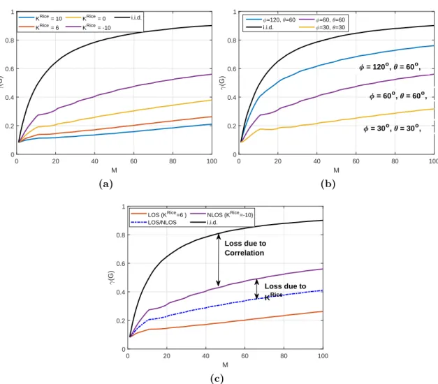
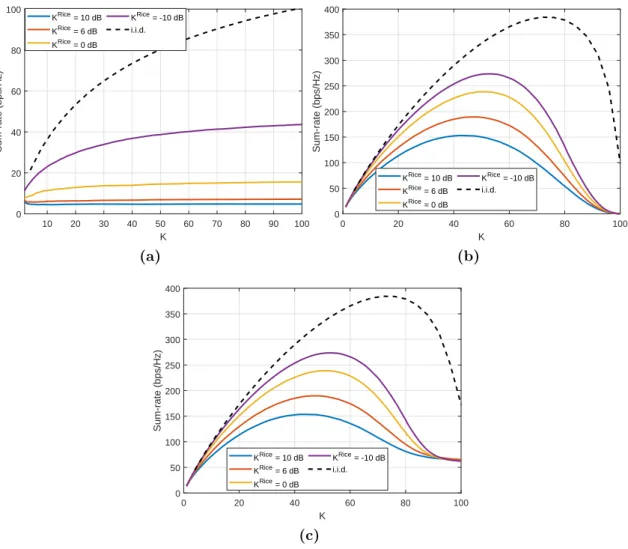
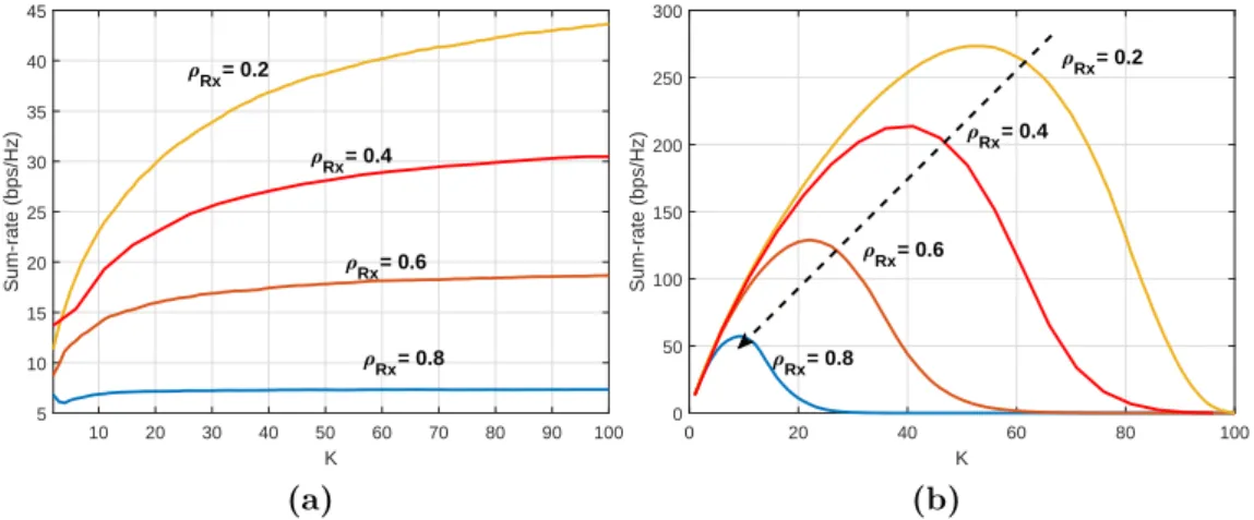
(16) Thèse de Frédéric Challita, Université de Lille, 2019. List of Figures. 2.8 2.9 2.10 2.11 2.12 2.13 2.14 2.15 2.16. 3.1 3.2 3.3 3.4 3.5. 3.6 3.7. 3.8 3.9 3.10 3.11 3.12. 3.13. Impact of (a) K Rice and (b) (∆θ,∆φ) on Gram’s power ratio. (c) Comparison between LOS, NLOS and LOS/NLOS scenarios. . . . . Block Diagram of the Massive MIMO DL System. . . . . . . . . . . (a) C(H) of SISO, MISO, SIMO, 4 × 4 MIMO and (b) C(H) for different MIMO configurations in i.i.d. channels. . . . . . . . . . . . Exemple of a transmission using ZF for two users. . . . . . . . . . . Comparison between MRT, ZF and MMSE for K = 12 and (a) M = 12 and (b) M = 32. . . . . . . . . . . . . . . . . . . . . . . . . . . . Massive MIMO SE for (a) MRT (b) ZF. . . . . . . . . . . . . . . . Massive MIMO SE for (a) 0 dB (b) 10 dB. . . . . . . . . . . . . . . The sum-rate capacity as a function of K: impact of K Rice . (a) MRT, (b) ZF and (c) MMSE. . . . . . . . . . . . . . . . . . . . . . . . . . Impact of correlation on the sum-rate capacity for K Rice = −10 dB as a function of K. 4 configurations of the geometrical model are considered giving correlation values ranging from 0.2 to 0.8. (a) for MRT and (b) for ZF. . . . . . . . . . . . . . . . . . . . . . . . . . Example of an Industry 4.0 automation cell. . . . . . . . . . . . . . Schematic of the created URA for 1.35, 3.5 and 6 GHz. . . . . . . . Schematic of the dual-polarized patch antenna at 1.35 GHz. . . . . a) Panoramic view of the industrial hall from the Tx point of view and b) Schematic from above of the distributed setup. . . . . . . . . Example of UE positions with metallic structures UE8 (a), totally obstructed UE11 (b), with concrete surroundings UE12 (c) and visible LOS UE5 (d). . . . . . . . . . . . . . . . . . . . . . . . . . . . . . . |h1,50,ψ (f )|2 and |h8,50,ψ (f )|2 for co- and cross-polarization links. . . The average received gain in co-polarization scheme for all UEs across the Tx array at (a) 1.35 GHz, (c) 3.5 GHz, (e) 6 GHz and the boxplot of average received gain in both polarizations displaying gain variations at (b) 1.35 GHz, (d) 3.5 GHz, (f) 6 GHz. . . . . . . . . . The median values of Bc,0.7 (a), K Rice (b) and ρT x (c) for the three studied frequency bands. . . . . . . . . . . . . . . . . . . . . . . . . Classification of UEs with a scatter plot of Bc and ρT x for (a) 1.35 GHz, (b) 3.5 GHz, (c) 6 GHz. . . . . . . . . . . . . . . . . . . . . . CDF of the XPD factor for LOS (UE 1), NLOS (UE 11) at (a) 1.35 GHz, (b) 3.5 GHz and (c) 6 GHz. . . . . . . . . . . . . . . . . . . . V{khk k2 } Channel hardening effect using (E{kh 2 2 for (a) LOS UE1, (b) OLOS k k }) UE 3 and (c) NLOS UE 11, as a function of M . . . . . . . . . . . . Receiver Spatial Correlation matrix RRx for all UEs averaged over frequencies: Co-polarization with (a) M = 32 and (c) M = 64, Crosspolarization with (b) M = 32 and (d) M = 64. . . . . . . . . . . . . Average spatial correlation ρRx evolution with M for (a) LOS scenario (b) NLOS and (c) total scenario. . . . . . . . . . . . . . . . . . . .. . 76 . 78 . 79 . 81 . 84 . 84 . 85 . 86. . 87 . 90 . 95 . 95 . 97. . 98 . 99. . 101 . 102 . 103 . 106 . 107. . 109 . 110. 16. © 2019 Tous droits réservés.. lilliad.univ-lille.fr.
(17) Thèse de Frédéric Challita, Université de Lille, 2019. List of Figures. 3.14 Gram’s Power Ratio γ(G) evolution with M for LOS and NLOS scenarios. The UE channels are normalized to remove the effect of channel gains imbalance. . . . . . . . . . . . . . . . . . . . . . . . 3.15 Gram’s Power Ratio γ(G) evolution with UE positions for (a) LOS, (b) NLOS scenarios and (c) Average γ(G) evolution in the total scenario. . . . . . . . . . . . . . . . . . . . . . . . . . . . . . . . . . . 3.16 Sum-rate capacity evolution with the SNR for (a) MRT, (c) ZF for M = 64 and the evolution with M for a SN R of 10 dB in (b) MRT and (d) ZF. The LOS and NLOS scenarios are compared. . . . . . 3.17 Sum-rate capacity evolution with the SNR for the total scenario with MRT, and ZF. The results are presented for M = 64. . . . . . . . . 3.18 Communication scheme with (a) Full co- or cross-polarized channel ˆ = 50. . . . . . . . with M = 100 and (b) Diversity scheme with M 3.19 Sum-rate capacity evolution with the SNR for (a) MRT, (c) ZF for NRF = 100 and the evolution with NRF for a SN R of 10 dB in (b) MRT and (d) ZF. . . . . . . . . . . . . . . . . . . . . . . . . . . . . Simplified preview of the method to estimate user channels with reduced feedback overhead. . . . . . . . . . . . . . . . . . . . . . . . 4.2 CDF of correlation values for any inter-element spacing in the array for LOS, NLOS and OLOS scenarios. . . . . . . . . . . . . . . . . 4.3 Colormap of the full CCM RT x for UE 1 (a), 3 (b) and 8 (c), respectively in LOS, OLOS and NLOS conditions. . . . . . . . . . . . . . 4.4 CDF of Tx correlation values in vertical plane (a) and horizontal plane (b) for different antenna spacing: 2d, 4d, 6d, 8d. In (c), the correlation values of the full correlation matrix is presented for all possible spacing d and in both directions x and z merged. . . . . . 4.5 Measured vs. Estimated transfer function for UE 8. . . . . . . . . . 4.6 Variation of β (in %) for different number of reference elements Mref - Impact of the number of reference antennas Mref on the computed channel capacity from estimated channels and for successive position of the UE. . . . . . . . . . . . . . . . . . . . . . . . . . . . . . . . 4.7 Number of pilot samples for TDD, FDD and the correlation-based approach for feedback overhead reduction. An example for K = 64 is considered and M varies from 64 to 256. . . . . . . . . . . . . . . 4.8 Switching architecture example S out of M . . . . . . . . . . . . . . 4.9 Investigated subset configurations from a URA. . . . . . . . . . . . 4.10 Antenna selection evaluation algorithm. . . . . . . . . . . . . . . . . 4.11 The average spatial correlation for the different configurations, showing all the draws, for S = 36. In (a) the total scenario and (b) LOS UEs as defined in Ch. 3. . . . . . . . . . . . . . . . . . . . . . . . .. . 112. . 113. . 115 . 116 . 118. . 120. 4.1. . 126 . 127 . 127. . 128 . 132. . 133. . . . .. 135 136 138 140. . 141. 17. © 2019 Tous droits réservés.. lilliad.univ-lille.fr.
(18) Thèse de Frédéric Challita, Université de Lille, 2019. List of Figures. 4.12 CDF of γ(G) for (a) LOS and (b) NLOS scenario. The 4 different configurations (S = 36) are presented as well as the i.i.d. curve for the sake of comparison. The evolution of γ(G) as a function of UE position is also presented in (c) and (d) for the LOS and NLOS scenario, respectively. . . . . . . . . . . . . . . . . . . . . . . . . . . . 142 4.13 Sum-rate capacity variation for ZF precoding with SN R for (a) LOS and (b) NLOS scenario. 3 values of S are considered: 9, 25 and 81, compared with the full-array performance. . . . . . . . . . . . . . . . 144 4.14 β (in %) variation with S for the LOS and NLOS scenarios with (a) MRT and (b) ZF. The BSS for different values of S is compared with the Sub-array. . . . . . . . . . . . . . . . . . . . . . . . . . . . . . . 145 6.1. NOMA associated to massive MIMO in highly correlated environments.154. B.1 Waterfilling algorithm principle. . . . . . . . . . . . . . . . . . . . . . 164 C.1 Convergence of the MLE estimator for different K Rice values. . . . . . 165 D.1 ρRx values for different elevation ∆θ and azimuth ∆φ angles (in o ) and different K Rice values: (a) -10 dB, (b) 0 dB, (c) 6 dB and (d) 10 dB. These parameters are set using the geometrical model. . . . . . D.2 ρT x,3λ/2 values for different elevation ∆θ and azimuth ∆φ angles (in o ) and different K Rice values: (a) -10 dB, (b) 0 dB, (c) 6 dB and (d) 10 dB. These parameters are set using the geometrical model. . . . D.3 CDF of the spatial correlation values ρi,j for all (i, j) combinations. The comparison is done for (a) LOS, NLOS scenarios of Ch. 3 and geometrical model for each case, (b) the total scenario with all UEs and (c) the correlation at Tx for inter-element spacing of 3λ/2 for LOS and NLOS UE. . . . . . . . . . . . . . . . . . . . . . . . . . . D.4 Comparison of the Gram’s power ratio dependence with M between measured and geometrical channels for the LOS and NLOS scenarios. The geometrical model was tuned using the parameters defined in the previous section. . . . . . . . . . . . . . . . . . . . . . . . . . . . .. . 167. . 168. . 169. . 170. E.1 Scattering parameter S11 in dB for the three frequencies (a) 1.35 GHz, (c) 3.5 GHz and (e) 6 GHz. Patch Gain in dB for the three frequencies (b) 1.35 GHz, (d) 3.5 GHz and (f) 6 GHz. . . . . . . . . . . . . . . . 172 E.2 Radiation pattern in azimuth cut for (a) 3.5 GHz, (b) 6 GHz and in elevation cut for (c) 3.5 GHz, (d) 6 GHz. . . . . . . . . . . . . . . . 173 E.3 Radiation pattern for co- and cross polarizations at (a) 3.5 GHz and (b) 6 GHz. . . . . . . . . . . . . . . . . . . . . . . . . . . . . . . . . . 174. 18. © 2019 Tous droits réservés.. lilliad.univ-lille.fr.
(19) Thèse de Frédéric Challita, Université de Lille, 2019. List of Tables. 1.1 1.2 1.3. Gaps and Challenges towards 5G. . . . . . . . . . . . . . . . . . . . . 29 Main Differences in PHY layer of LTE and 5G-NR. . . . . . . . . . . 30 Mobile Technologies for 5G. . . . . . . . . . . . . . . . . . . . . . . . 31. 2.1 2.2. Model parameters for channel hardening simulations. . . . . . . . . . 74 Model parameters for favorable propagation conditions simulation. . . 75. 3.1 3.2. . 92. Advances in massive MIMO Channel Measurements. . . . . . . . . Radio Channel Sounding Parameters and different Tx array dimensions. . . . . . . . . . . . . . . . . . . . . . . . . . . . . . . . . . . 3.3 Main Parameters of the antennas. . . . . . . . . . . . . . . . . . . . 3.4 Experimental Vs Theoretical Friis Gain and NLOS relative gain to UE 1 for the three frequencies. . . . . . . . . . . . . . . . . . . . . . 3.5 Statistics of key channel parameters over the Tx array at the studied frequencies for LOS UE 1, OLOS UE 3 and NLOS UE 11. . . . . . 3.6 Cross-correlation between channel parameters. . . . . . . . . . . . . 3.7 Median XPD value at the three frequencies for LOS and NLOS scenarios. . . . . . . . . . . . . . . . . . . . . . . . . . . . . . . . . . . 3.8 Minimum number of Tx antennas for ρt,Rx = 0.3. . . . . . . . . . . 3.9 Summary of Sum-rate capacity results with M = 64 and SN R = 20 dB. . . . . . . . . . . . . . . . . . . . . . . . . . . . . . . . . . . . . 3.10 UEs polarization maps using strategy 1 and 2. . . . . . . . . . . . . 3.11 Summary of sum-rate capacity results with the proposed diversity schemes. . . . . . . . . . . . . . . . . . . . . . . . . . . . . . . . . . 4.1 4.2. 4.3. . 94 . 95 . 100 . 104 . 104 . 105 . 111 . 116 . 119 . 120. β (in %) of the sum-rate capacity with MRT and ZF for different Mref .134 Variation of γ(G) with respect to the full-array (in %) with S for LOS and NLOS scenarios. Three configurations are compared: Full, Sub-Array and BSS. . . . . . . . . . . . . . . . . . . . . . . . . . . . 143 Variation of β (in %) with S for LOS and NLOS. Two configurations are compared: BSS with MRT and ZF. . . . . . . . . . . . . . . . . . 146 19. © 2019 Tous droits réservés.. lilliad.univ-lille.fr.
(20) Thèse de Frédéric Challita, Université de Lille, 2019. List of Tables. 4.4. Variation of β (in %) with S for the total scenario. Two configurations are compared: BSS with MRT and ZF and the corresponding sumrate capacity values are given. . . . . . . . . . . . . . . . . . . . . . . 146. 20. © 2019 Tous droits réservés.. lilliad.univ-lille.fr.
(21) Thèse de Frédéric Challita, Université de Lille, 2019. List of Publications Accepted Papers in Peer-Review Journals J1 F. Challita, M. Martinez-Ingles, M. Liénard, J. Molina-García-Pardo and D. P. Gaillot, “Line-of-Sight Massive MIMO Channel Characteristics in an Indoor Scenario at 94 GHz”, in: IEEE Access, vol. 6, pp. 62361-62370, 2018. J2 F. Challita, P. Laly, M. Liénard, E. Tanghe, W. Joseph and D. P. Gaillot, “Hybrid virtual polarimetric massive MIMO measurements at 1.35 GHz”, in: IET Microwaves, Antennas and Propagation- Special Session, 2019. J3 M. Yusuf, E. Tanghe, F. Challita, P. Laly, D. P. Gaillot, M. Liénard, L. Martens and W. Joseph, “Stationarity Analysis of V2I Radio Channel in a Suburban Environmen”, in: IEEE Transactions on Vehicular Technology. (Accepted) J4 F. Challita, VMR.Peñarrocha, L. Rubio, J. Reig, LJ. Llácer, JP. García, J. Molina-García-Pardo, M. Liénard and DP. Gaillot, “On the contribution of Dense Multipath Components in an intra-wagon environment for 5G mmW Massive MIMO channels”, in: IEEE Antennas and Wireless Propagation Letters. J5 F. Challita, P. Laly, M. Liénard, E. Tanghe, M. Yusuf, W. Joseph and D. P. Gaillot, “Channel Correlation-based approach for feedback overhead reduction in massive MIMO”, in: IEEE Antennas and Wireless Propagation Letters, 2019.. Papers Under Review J6 F. Challita, J. Molina-García-Pardo , M. Liénard, and D. P. Gaillot, “Evaluation of an antenna selection strategy for reduced massive MIMO complexity”, in: Radio Science. 21. © 2019 Tous droits réservés.. lilliad.univ-lille.fr.
(22) Thèse de Frédéric Challita, Université de Lille, 2019. List of Publications. Accepted Papers in Peer-Review International Conferences C1 F. Challita, P. Laly, M. Liénard, D. P. Gaillot, J. M. Molina-Garcia-Pardo and W. Joseph, “MIMO in Tunnel: Impact of Polarization and Array Orientation on the Channel Characteristics”, 2018 IEEE Radio and Antenna Days of the Indian Ocean (RADIO), Grand Port, 2018, pp. 1-2. C2 F. Challita, P. Laly, M. Liénard, D. P. Gaillot, P. Degauque, W. Joseph, “Experimental Study of Depolarization and Antenna Correlation in Tunnels in the 1.3 GHz Band”, 2019 26th International Conference on Telecommunications (ICT), Ha Noi, Vietnam, pp. 1-5. C3 M. Yusuf, E. Tanghe, F. Challita, P. Laly, D. P. Gaillot, M. Liénard, B. Lannoo, R. Berkvens, M. Weyn, L. Martens and W. Joseph, “Experimental Characterization of V2I Radio Channel in a Suburban Environment”, 2019 13th European Conference on Antennas and Propagation (EuCAP), Krakow, Poland, 2019, pp. 1-5. C4 F. Challita, M. Martinez-Ingles, M. Liénard, J. Molina-García-Pardo and D. P. Gaillot, “Evaluation of an Antenna Selection Strategy for Reduced Massive MIMO Complexity”, 2018 12th European Conference on Antennas and Propagation (EuCAP 2018) ,London, UK, pp.1-5. C5 F. Challita, M. Yusuf, E. Tanghe, P. Laly, M. Liénard, W. Joseph and D. P. Gaillot,“Impact of Polarization Diversity in Massive MIMO for Industry 4.0”, 2019 European Conference on Networks and Communications (EuCNC) 2019, Valencia, Spain, pp. 1-5.. IRACON-COST1 Conference P1 F. Challita, M. Martinez-Ingles, M. Liénard, J. Molina-García-Pardo and D. P. Gaillot, “Line-of-Sight Massive MIMO Channel Characteristics in an Indoor Scenario at 94 GHz”, 4th MCM and 4th Technical meeting, Lund, Sweden. P2 F. Challita, M. Martinez-Ingles, M. Liénard, J. Molina-García-Pardo and D. P. Gaillot, “Evaluation of an Antenna Selection Strategy for Reduced Massive MIMO Complexity”, 5th MCM and 5th Technical meeting, Cartagena, Spain. 1. The Inclusive Radio Communications (IRACON) COST ACTION CA15104 aims to introduce novel design and analysis methods for 5G and beyond-5G radio networks. The main goal of working group 1 is to develop accurate radio channel models for inclusive deployment scenarios at different frequencies and co-develop antenna systems that can cope with the the targeted deployments.. 22. © 2019 Tous droits réservés.. lilliad.univ-lille.fr.
(23) Thèse de Frédéric Challita, Université de Lille, 2019. List of Publications. P3 F. Challita, P. Laly, M. Liénard, E. Tanghe, W. Joseph and D. P. Gaillot, “Impact of polarization in hybrid virtual polarimetric massive MIMO measurements at 1.35 GHz”, 6th MCM and 6th Technical meeting, Cartagena, Spain. P4 F. Challita, E. Tanghe, , P. Laly, M. Liénard, W. Joseph and D. P. Gaillot, “Massive MIMO for Industrial Scenarios : Measurement-Based Polarimetric Analysis”, 9th MCM and 9th Technical meeting, Dublin, Ireland. P5 M. Yusuf, E. Tanghe, F. Challita, P. Laly, D. P. Gaillot, M. Liénard, B. Lannoo, R. Berkvens, M. Weyn, L. Martens and W. Joseph, “Experimental Characterization of V2I Radio Channel in a Suburban Environment”, 9th MCM and 9th Technical meeting, Dublin, Ireland. P6 M. Martinez-Ingles, F. Challita, D. P. Gaillot, JP. García, J. Molina-GarcíaPardo, “1-100 GHz Deterministic and Experimental Indoor Channel Modeling”, 9th MCM and 9th Technical meeting, Dublin, Ireland.. Other Participation in European School of Antennas (ESoA) 2017- Université Catholique de Louvain (Summer School) and ranked first in the final exam.. 23. © 2019 Tous droits réservés.. lilliad.univ-lille.fr.
(24) Thèse de Frédéric Challita, Université de Lille, 2019. © 2019 Tous droits réservés.. lilliad.univ-lille.fr.
(25) Thèse de Frédéric Challita, Université de Lille, 2019. Chapter. 1. General Introduction and Motivations Chapter Outline In this introductory chapter, a general overview of 5G is presented in Sec. 1.1 while Sec. 1.2 focuses on the main features, use-cases and enabling technologies. A brief introduction of multi-antenna systems is given in Sec. 1.3. Massive MIMO (multipleinput multiple-output) systems, their key features, systems architecture and channel estimation are detailed in Sections 1.4, 1.5 and 1.7. Section 1.6 gives a summary of massive MIMO testbeds, first trials and challenges published in the literature. Lastly, Sections 1.8 and 1.9 present the different contributions of this work as well as the thesis organization, respectively. Other contributions during these 3 years of Ph.D. are listed in Sec. 1.10.. 1.1 1.1.1. Introduction: Overview of The 5th Generation 5G: Evolution or Revolution ?. Mobile connectivity has become not only essential but a necessity for many network users. Technological advances and computer abilities are needed to provide faster, smarter and safer wireless networks [2]. The domain of application is wide and not limited to mobile devices and cellular networks [3] but also includes connected machines in industrial setups, vehicular communications (vehicle-to-everything or V2X) [4] and smart cities [5, 6]. Network architectures and generations have also evolved from the first digital generation (GSM or Global System for Mobile Communications) to the most recent generation network connectivity 4G (LTE or Long Term Evolution). The next 5 years are projected to supply unprecedented data rates and networks efficiency should follow along. The number of mobile subscribers is growing rapidly and the demand for more bandwidth (BW) and higher data rates continues to increase as reported by CISCO [7]. This explosion of mobile applica25. © 2019 Tous droits réservés.. lilliad.univ-lille.fr.
(26) Thèse de Frédéric Challita, Université de Lille, 2019. 1.1. Introduction: Overview of The 5th Generation. tions and adoption of mobile connectivity alongside the need for higher data rates, green energies and cutting-edge applications, is fueling the growth of 4G deployments, soon to be followed by 5G systems. All these points and many others lead to one conclusion: the need for cutting edge technologies [8] to support consumer usage trends and keep cost efficient solutions in terms of infrastructure. From this discussion, it appears that 5G would eventually be more of a revolution than an evolution of 4G, changing the way the world is perceived. However, although 5G is being marketed as a brand new technology, it will not be built from scratch [9, 10] and hybrid non-standalone configurations using both 5G and 4G technologies will co-exist.. 1.1.2. Initial Vision: Use-cases for 5G New Radio. With the increasing requirements upon the new 5G communication standards, a new radio (NR) interface and radio access network (RAN) are being developed. 5G NR is the name that the third generation partnership project (3GPP) chose for 5G when Release 15 was announced. NR is the equivalent of LTE for 4G or UMTS technology for 3G technology. 5G NR’s goal is to meet the performance requirements set by the international telecommunication union (ITU) for the year 2020. More specifically, recommendation ITU-T Y.3101 presents distinguishing features and requirements of the international mobile telecommunications 2020 (IMT-2020) for 5G networks. Promising technologies capable of fulfilling the gap from previous generations are sought. An overview of the NR interface standard under development by 3GPP is available in [11] with preliminary specifications for Release 15 approved in December 2017 [12]. Release 16 will provide further specifications for the second phase. The most central use-cases are not final and still being discussed both in ITU, 5G-PPP [13], the METIS project [14] and in 3GPP [12]. The main use cases to be supported span three different dimensions: enhanced mobile broadband (eMBB), massive machine type communications (mMTC) and ultra-reliable low latency communications (URLLC). Additional use-cases may naturally emerge in time with the evolution of the physical layer radio interface [15]. 1.1.2.1. Use-Cases. Enhanced Mobile Broadband (eMBB): Can be defined as the feature of 5G as the most relevant evolution of 4G. It is a datadriven use-case enabling new applications such as virtual reality (VR). Improved spectral efficiencies, cell-edge data rates and coverage, amongst other requirements, define the shape of eMBB in 5G networks. The relevant 5G requirements are: • Peak throughput: 20 Gbps in Downlink (DL), 10 Gbps in Uplink (UL). • Experienced data rates (5th percentile user throughput): 100 Mbps (DL), 50 Mbps (UL). 26. © 2019 Tous droits réservés.. lilliad.univ-lille.fr.
(27) Thèse de Frédéric Challita, Université de Lille, 2019. Chapter 1. General Introduction and Motivations • Area capacity (e.g. indoor hotspot): 10 Mbps/m2 . • User plane latency: 4 ms Massive Machine Type Communications (mMTC): Industry 4.0 IoT requires massive connectivity where tens of billions of interconnected low-cost devices and sensors communicate [16]. Recent advancements on machine-to-machine (M2M) communications in 4G networks are presented in [17]. This is being labeled as the fourth industrial revolution or Industry 4.0. There are many advantages brought by 5G cutting edge technologies for industrial automation scenarios in the drive for Industry 4.0 [18]. In [19], challenges and solutions for M2M communications are depicted. Relaxed data rates constraints are sought compared to eMBB but other strict requirements are still to be fulfilled: • Density: 1 Million devices/km2 . • Wide Coverage: 164 dB Maximum Coupling Loss (MCL). • Device battery life: 10-15 years. Ultra-Reliable Low Latency Communications (URLLC) Critical applications (e.g. Intelligent V2X, remote surgery, smart grids, etc.) define very stringent latency and reliability requirements. For this ultra-reliable and low latency area communications, specific requirements are needed [20, 21]: • Latency: less than 1 ms. • Reliability : 99.999%. • Control plane latency: tens of ms. • User plane latency: less than 0.5 ms (one-way UL and DL). • Mobility interruption time: 0 ms. 1.1.2.2. Multi-Layer Spectrum. Globally harmonized spectrum is needed for 5G systems to ensure the different requirements and satisfy future expectations and potential capabilities. 5G network deployments are converging to new frequency bands: 3.5 GHz (16% of total number of trials) and 24.25-27.5 GHz (19% of total number of trials) frequency ranges [22], two new frequencies to the cellular network industry. For instance, in France, Arcep (telecom regulator) announced it was planning to issue temporary frequency authorizations (in the 3.5 GHz band [3400 – 3800 MHz]) to develop 5G in France [23]. Also, it is expected that some applications of 5G networks will require very 27. © 2019 Tous droits réservés.. lilliad.univ-lille.fr.
(28) Thèse de Frédéric Challita, Université de Lille, 2019. 1.1. Introduction: Overview of The 5th Generation. wide contiguous blocks of bandwidths (up to several GHz) to support high overall system capacities. To this end, high carrier frequencies (> 6 GHz) need to be considered. Maintaining a sustainable spectrum management environment is also critical for long term investments even if new techniques are envisaged. In Release 15 of 5G NR, two frequency ranges are defined [24]: • 450 MHz - 6 GHz or the sub-6 GHz bands. • 24.25 GHz - 52.6 GHz or the millimetr wave (mmW). This multi-layer spectrum approach is vital to address the wide range of usage scenarios. The sub-6 GHz band is also divided into two parts as indicated below. According to Huawei in [25], 3 layers can be defined: • Below 2 GHz: delivers high coverage for wide areas and deep indoor scenarios, useful for mMTC [26] to help support IoT services. It is also needed to extend high speed mobile broadband coverage across urban, suburban and rural areas. Mobile spectrum in this range can be used in the future for some use-cases. The European Commission has already expressed its wish to use the 700 MHz band to support 5G services in Europe. Similarly, the FCC (Federal Communications Commission) indicated that the 600 MHz band could be used in the United States and several other countries. Furthermore, the ITU is considering additional spectrum for mobile broadband from in 2023 (470-694 MHz), a good timing for 5G services. • From 2 to 6 GHz (C-band): The 3.3-4.2 and 4.4-5 GHz ranges deliver the best compromise between wide coverage and spectral efficiency making them attractive for eMBB. The 3.3-3.8 GHz range is almost globally harmonized and used as the basis for initial commercial 5G services. A number of countries are exploring whether a portion of other bands could be used such as 3.8-4.2 GHz and spectrum in the 4-5 GHz range, in particular 4.8-4.99 GHz. The availability of at least 100 MHz BW per 5G network alongside the potential of massive MIMO will potentially boost throughputs (peak, average and celledge) with relatively affordable complexity. • Above 6 GHz: delivers extremely high data rates (super data layer), and is widely recognized as a key component for hotspot areas, fixed broadband and fiber-like connectivity. mmW frequencies have particular propagation characteristics and are more sensible to blockage than lower frequencies. Accurate channel models and characteristics are needed to understand the different mechanisms at these frequency ranges [27]. The targeted spectrum above 6 GHz is expected to handle a mixture of licensed and unlicensed mobile bands. 24.25-29.5 GHz, 31.8-33.4 GHz, 37-43.5 GHz, 45.5-50.2, GHz, 50.4-52.6 GHz, 66-76 GHz and 81-86 GHz bands should be agreed in WRC-19. Studies concerning mmW mobile communications for 5G cellular networks can be found in [28]. The authors presented some measurement results at 28 and 38 GHz 28. © 2019 Tous droits réservés.. lilliad.univ-lille.fr.
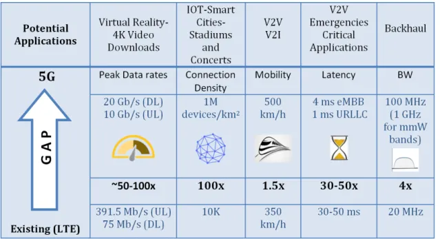
(29) Thèse de Frédéric Challita, Université de Lille, 2019. Chapter 1. General Introduction and Motivations. frequencies showing the possibility of employing steerable directional antennas at base stations (BS) and mobile devices. In [29], a theoretical feasibility study and prototype results on mmW beamforming are presented. In [30], the authors study the feasibility of spatial multiplexing and maximum ratio transmitter for mmW large MIMO. From a cell point of view, this classification can be further generalized [9]: • Macro-Cell : < 1 GHz: full coverage (rural scenarios and deep indoor). • Dense urban: from 2 to 6 GHz: high date rates. • Small cell 28/39 GHz (> 6 GHz generally): 10 Gbps hotspots. • Ultra small cell: future mmW options and very high data rates.. 1.1.3. Gaps and Challenges. The wireless industry has witnessed rapid growth in the last few decades. Nonetheless, many gaps and challenges should be addressed for the full development of 5G. Table 1.1 presents some differences between LTE and 5G, and the corresponding targeted applications and use-cases.. Table 1.1: Gaps and Challenges towards 5G. Other requirements related to technical performance for 5G radio interface such as energy efficiency (10 times longer battery life for low-power M2M), core network technologies, outage probability, interruption time, etc. can be found in [31, 26, 32, 33]. Spectrum policies and regulatory issues as already discussed need to be tackled 29. © 2019 Tous droits réservés.. lilliad.univ-lille.fr.
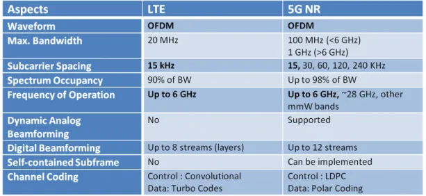
(30) Thèse de Frédéric Challita, Université de Lille, 2019. 1.2. Impacting technologies of 5G. before a worldwide deployment [34, 35]. NR Phase 1 and LTE share some common technical aspects such such as OFDM (orthogonal frequency-division multiplexing). However, PHY layer of NR phase 1 is scalable and supports new transmission modes in digital beamforming. This is illustrated in Table 1.2.. Table 1.2: Main Differences in PHY layer of LTE and 5G-NR.. 1.2. Impacting technologies of 5G. In order to satisfy the different requirements for 5G systems, improvements of existing technologies and emerging techniques should be evaluated [3, 36]. The 5 main impacting technologies of 5G are: • mmW: A gold mine of spectrum and contiguous blocs of bandwidths. • Cloud-based radio access network (C-RAN): centralized baseband units (BBU) are separated from remote radio heads (RRHs). Different RRHs are connected to a centralized cloud with all the signal processing [37, 38]. • M2M communications and Industry 4.0: support of a large number of low-rate devices at very low latency data-transfer. • Device-centric architectures: small-cells (micro, femto) in a heterogeneous network (HETNETs), traffic offload, better coverage, etc. • Massive MIMO: allowing the densification of BS or access points (AP) by deploying massive Tx arrays capable of multiplexing many user equipments (UEs) in the same time-frequency resource. It is a cutting-edge technology capable of filling the gap for many 5G systems requirements [32] by increasing system capacity of new wireless systems [39].. 30. © 2019 Tous droits réservés.. lilliad.univ-lille.fr.
(31) Thèse de Frédéric Challita, Université de Lille, 2019. Chapter 1. General Introduction and Motivations. Many demonstrations have already highlighted the effectiveness of massive MIMO systems implementation, mostly for cellular communications, indoor scenarios, etc. and will be discussed later. Table 1.3 lists the different technologies and aspects of 5G NR highlighting the emergence of massive MIMO .. Table 1.3: Mobile Technologies for 5G.. 1.2.1. Massive MIMO: Why Now ?. Multi-antenna systems are a must to address the different requirements of 5G-NR. Extra antennas used in massive MIMO help focusing energy into ever smaller regions of space to bring huge improvements in throughput and radiated energy efficiency [40]. Other benefits such as cheaper parts, lower latency, reliability, amongst others, make massive MIMO an interesting candidate for 5G. System throughput, defined as the sum of data rates delivered to all users in a given cell and measured in bits per second (bits/s or bps), is a key parameter for performance evaluation. Throughput is directly related to BW and spectral efficiency (SE) as illustrated in Eq. 1.1. The SE measured in bits/s/Hz (bps/Hz), is a deterministic number and gives direct insight into expected data rates for a given system: T hroughput(bits/s) = BW (Hz) × SE(bits/s/Hz).. (1.1). The maximum SE is determined by the channel capacity defined by Claude Shannon is his seminal paper from 1948 [41]. Clearly, in order to increase data rates, higher bandwidths are needed and/or better SE. Due to congestion in cellular frequencies (below 6 GHz), the second option is more adapted for this frequency range. For mmW bands, the first option can be easily applied because of large contiguous blocs of spectrum. In the following, some key points address the “Why Now ” question: 31. © 2019 Tous droits réservés.. lilliad.univ-lille.fr.
(32) Thèse de Frédéric Challita, Université de Lille, 2019. 1.3. Multi-antenna System Communications. • Congestion of macro networks, base sites will run out of capacity by 2020 for sub-6 GHz spectrum: capacity requirements fulfilled by spatial multiplexing in massive MIMO. • Large BW above 6 GHz but complicated propagation conditions : coverage requirements fulfilled by high gain adaptive arrays in massive MIMO. • Massive MIMO is now supported (primary versions) in release 13-14 for LTE and 15 for 5G-NR: 3GPP specifications support. • Low cost and high efficiency components for active antenna arrays are becoming technically and commercially feasible: Technology capability. • In Rel. 15-NR, diversity schemes are not explicitly supported: Spatial multiplexing is becoming more and more essential.. 1.3. Multi-antenna System Communications. Multiple antennas at either both ends or one end of the communication link have been widely used in wireless systems to address different challenges such as link reliability (diversity techniques) or SE (multiplexing techniques). In order to understand massive MIMO, MIMO and MU-MIMO are first introduced.. 1.3.1. MIMO Communications. MIMO systems gained considerate attention for the past decades [42, 43] and are now incorporated into most of the new generation wireless standards. Transmission with MIMO antennas is a well-known method to overcome fading and enhance link reliability: this is categorized as diversity. Also, simultaneous communication of multiple data streams over the same radio channel by exploiting the multipath nature of the radio channel started a considerate evolution in data rates and system capacity. This paves the way for a wide variety of use-cases and applications. More recently, MIMO has been applied to power line communications (PLC) [44, 45, 46]. 1.3.1.1. Fundamentals and system model. A simple system model with M transmitting antennas (Tx) and N receiving antennas (Rx) is presented in Fig. 1.1. The N ×M channel matrix H contains the channel coefficients linking each Tx antenna to each Rx antenna of a single-user (SU). For diversity schemes, each Rx antenna combines the Tx signals which coherently add up to provide signal-to-ratio (SNR) gains on one hand, or to increase reliability on the other hand. MIMO systems have the capability to multiply systems throughput by min(M, N ) in ideal rich multipath conditions: this is spatial multiplexing. The memoryless MIMO flat fading channel (narrowband model) is given by : y = Hx + n,. (1.2). 32. © 2019 Tous droits réservés.. lilliad.univ-lille.fr.
(33) Thèse de Frédéric Challita, Université de Lille, 2019. Chapter 1. General Introduction and Motivations. Figure 1.1: SU-MIMO system model. • H is the N × M complex channel matrix given by :. . h11 h21 . . .. h12 h22. ... hN 1 hN 2. . . . . h1M . . . h2M .. ... . . . . hN M. • hij is the complex channel gain between Tx and Rx elements with i = 1, ..., M and j = 1, , ..., N • x is the M × 1 complex transmitted signal vector • y is the N × 1 complex received signal vector • n is the N × 1 complex additive noise signal vector with variance σn2 .. 1.3.2. Multi-User MIMO. MU-MIMO have been attracting considerable interest [47]-[48] and is still a hot topic for wireless communication systems [49]-[50]. A BS or AP equipped with M antennas (up to 16) communicating with a number of distributed users K (equipped with N ≥ 1 antennas) falls into the MU-MIMO systems category. Generally, the transmitter should be equipped (as a minimum) with as many antennas as the total number of served users antennas. A sketch of the MU-MIMO (multi-user MIMO) scenario with K users equipped with N = 1 is illustrated in Fig. 1.2. 33. © 2019 Tous droits réservés.. lilliad.univ-lille.fr.
(34) Thèse de Frédéric Challita, Université de Lille, 2019. 1.3. Multi-antenna System Communications. Figure 1.2: MU-MIMO scenario. The research on MU-MIMO is not recent and have witnessed some impactful array processing papers [51, 52, 53, 54]. These systems can harmonize the high capacity achieved using standard MIMO processing techniques with the benefits of space-division multiple access (SDMA) for which the spatial degrees of freedom (DoF) are used as multiplexing dimension. This technique supports multiple connections on a single channel where different users are spotted by their spatial signatures inside the network. SDMA also helps mitigate the effects of adjacent cell interference. 1.3.2.1. Advantages of MU-MIMO. Traditionally, the time-frequency resources are divided into resource blocks (RB) and one user is active per RB for which the SISO (single-input single-output) SE is quantified as log2 (1 + SN R) with SN R an average signal-to-noise ratio. In a suitable and rich multipath environment, multiple users can be simultaneously assigned multiple parallel streams. The total SE is thus scaled up by a factor G, known as Multiplexing Gain, the number of potential parallel streams. The total SE becomes G log2 (1 + SN R) for an interference-free case. This is a general approach to quantify the SE, details on power allocation and other systems aspect are given in Ch. 2. The need to harvest multiplexing gains has motivated the effort to switch from MIMO systems to MU-MIMO. It is noteworthy that SDMA does not require multiple antenna at the UE [55]. The MU-MIMO main advantages are listed below: • Possibility of using one antenna at Rx for each user: less constraints on the physical size of UE and cost requirements. • MU-MIMO is better equipped than MIMO to overcome most of propagation limitations such as ill-conditioned channels or strong line-of-sight (LOS) by using advanced scheduling schemes. 34. © 2019 Tous droits réservés.. lilliad.univ-lille.fr.
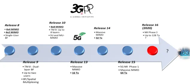
(35) Thèse de Frédéric Challita, Université de Lille, 2019. Chapter 1. General Introduction and Motivations. • Enhanced sum-rates inside a given cell: better use of spectrum resources. However, these advantages come at a price: • MU interference can be mitigated through precoding (widely discussed in Ch. 2) and cancellation techniques such as ML (Maximum Likelihood) detection for UL [56], dirty paper coding (DPC) [57, 58] for DL or interference alignment [59, 60]. Some approaches are based on beamforming techniques such as in [61, 62]. • Availability of channel state information at the transmitter (CSIT) is challenging especially in high mobility scenarios. • User scheduling and resource allocation schemes lead to an increase in implementation complexity.. 1.3.3. Evolution of multi-antenna systems with 3GPP. Multiple antennas can increase capacity and reliability but also provide spatial resolvability, spatial DoF for multiple users to share and higher SE. MIMO systems have evolved lately to include MU-MIMO systems (via the introduction of new transmission modes TM) before the arrival of massive MIMO [63]. This transition was motivated by many factors: • In the 1-6 GHz range of cellular communication, the number of antennas that can be deployed in compact user terminals is limited. • The wireless channel to a given terminal can have, in some configurations or scenarios, few contributing paths, limiting the ability to send parallel data streams. • Advanced signal processing schemes are sometimes needed in point to point MIMO to detect multiple streams. • For MU-MIMO, users should be spatially well-separated to avoid co-channel interference. • Small-scale fading can still affect the link reliability. • Massive MIMO can be a solution to focus, in an efficient manner, the energy towards the intended users. The following figure illustrates the evolution of multi-antenna systems under the scope of 3GPP standards and releases.. 35. © 2019 Tous droits réservés.. lilliad.univ-lille.fr.
(36) Thèse de Frédéric Challita, Université de Lille, 2019. 1.4. Massive MIMO: Massive Breakthrough. Figure 1.3: 3GPP Releases-From MIMO to massive MIMO. This figure displays the evolution from Release 8 to the up-coming Release 16.. 1.4 1.4.1. Massive MIMO: Massive Breakthrough History and Brief Introduction. The massive MIMO concept was first mentioned in the seminal paper: “Noncooperative Cellular Wireless with Unlimited Numbers of Base Station Antennas” [64] by Thomas Marzetta, published in 2010. This paper only talks about MU-MIMO systems with very large antenna arrays, but over the years, massive MIMO became a catchy term in all the published scientific papers. From this paper, it is understood that massive MIMO is a form of MU-MIMO, an asymptotic extension where M is very large and many UEs are simultaneously served (see Fig. 1.4). The transition from MIMO, MU-MIMO to massive MIMO, according to IEEE, is a clean break with current practice through the use of a large excess of service Tx antennas over active terminals. Generally speaking, the receivers (UEs, machines, industrial robots, etc.) in 5G use-cases are equipped with one antenna [9, 22, 25]. Transmission signals are adjusted by the physical layer using phase/gain control. The basic information, theoretical aspects and limits were presented in early works such as [65]-[66]. Massive MIMO is generally defined as “useful and scalable version of MU-MIMO” [67], or “a MU-MIMO system with M antennas and K users per BS. The system is characterized by M K and operates in time-division duplexing (TDD) mode (discussed later) using linear UL and DL processing” [68]. 36. © 2019 Tous droits réservés.. lilliad.univ-lille.fr.
(37) Thèse de Frédéric Challita, Université de Lille, 2019. Chapter 1. General Introduction and Motivations. Figure 1.4: Overall Massive MIMO System. These definitions cover most systems but are very general. In order to bring out the characteristics of such systems, some essential caracteristics covering the definition of massive MIMO are given hereafter. Massive MIMO:. • is an extensive raise in the number of transmitting antennas M packed into an array (see Fig. 1.5), • relies on the spatial dimension to form orthogonal sub-channels and simultaneously serve K users, • communicates over a channel with favorable propagation conditions, • benefits from channel hardening provided by the large number of antennas, • Uses TDD relying on channel reciprocity and UL pilots to obtain channel state information (CSI). Different antenna array geometries for the Tx are presented in Fig. 1.5 from [69]. Mostly recognized, the URA (uniform rectangular array) because of its horizontal and vertical aperture and the possibility of adjusting both elevation and azimuth angles. For instance, vertical alignment of the array elements is beneficial for users on different floors using elevation beamforming as shown in Fig. 1.6. 37. © 2019 Tous droits réservés.. lilliad.univ-lille.fr.
(38) Thèse de Frédéric Challita, Université de Lille, 2019. 1.4. Massive MIMO: Massive Breakthrough. Figure 1.5: Different Array Configurations: a) Linear, b) Rectangular and c) Cylindrical (Lund University).. Figure 1.6: Massive MIMO in the elevation and azimuth domain. 38. © 2019 Tous droits réservés.. lilliad.univ-lille.fr.
Figure
+7
Documents relatifs