Pépite | Lois stables généralisées et lois stables libres

Texte intégral

(1)Thèse de Min Wang, Université de Lille, 2019. École Doctorale Sciences Pour l’Ingénieur Laboratoire Paul Painlevé. Thèse présentée pour l’obtention du. Diplôme de doctorat de l’Université de Lille Spécialité: Mathématiques Generalized stable distributions and free stable distributions Lois stables généralisées et lois stables libres par Min Wang Soutenue le 7 juin 2019 devant le jury composé de: Nizar Demni. Université de Rennes. Nathalie Eisenbaum Sorbonne Université. Rapporteur Examinateur. Uwe Franz. Université de Franche-Comté Examinateur. Mylène Maïda. Université de Lille. Examinateur. Thomas Simon. Université de Lille. Directeur. Rapporteur absent à la soutenance: Alexey Kuznetsov York University. © 2019 Tous droits réservés.. lilliad.univ-lille.fr.

(2) Thèse de Min Wang, Université de Lille, 2019. Thèse préparée au Laboratoire Paul Painlevé (UMR CNRS 8524) Université de Lille Cité Scientifique 59 655 Villeneuve d’Ascq CEDEX grâce à un financement du Labex CEMPI. © 2019 Tous droits réservés.. lilliad.univ-lille.fr.

(3) Thèse de Min Wang, Université de Lille, 2019. In memory of my father, Tian-Shun.. © 2019 Tous droits réservés.. lilliad.univ-lille.fr.

(4) Thèse de Min Wang, Université de Lille, 2019. © 2019 Tous droits réservés.. lilliad.univ-lille.fr.

(5) Thèse de Min Wang, Université de Lille, 2019. Acknowledgment I am using this opportunity to express my gratitude to many people who helped me from different aspects. First of all, I would like to thank my supervisor, Professor Thomas Simon, for his guidance and constant help. During these years, Professor Simon has shared with me much of his deep knowledge in probability. He is always patient, smiling and kind to his students. I will forever cherish the memory of working with him. It is my honour that Professor Alexey Kuznetsov and Professor Nizar Demni have accepted to review my thesis. I would like to thank them for their careful reading and listing some corrections in the previous version. I would also like to thank Professor Uwe Franz, Professor Mylène Maïda and Professor Nathalie Eisenbaum for their acceptance to be members of the examining commission. I sincerely thank Professor Uwe Franz and Professor Mylène Maïda for their letters of recommendation which helped me get a postdoctoral position in Tsinghua University. I want to thank Mylène for answering my questions. I am also grateful for the kind invitations of Uwe and Dieter Mitsche to visit Université de Franche-Comté and Université Lyon 1, respectively. I warmly thank Professor Quanhua Xu, who has chatted with me several times for my future plan when I was an undergraduate, and thanks to him, I had the chance to study in France. The same gratitude should also be expressed to Professor Guoting Chen, who has helped me a lot during my studies in Lille. I thank many colleagues in my laboratory, such as Alexandre, Gaia, Stefana, Jimena, Clément, Ivan, Giulio, Duc-Nam, Angelo, Anto, Aya, Sheng-Chi, . . . , for the friendly and relaxing atmosphere we create together. I would like to thank Alexandre for correcting my french in daily conversations. I would also like to thank my Chinese friends, such as Enhui, Shuie, Bingyu, for many small talks we had which made me happy. I would like to express my thanks to the librarians, Omar and Hélène, for their kindly help of finding articles. I am especially grateful to my mother, for her selfless love and constant encouragement. Last but not least, I would like to thank my husband, Haowu, who understands all my tears and laughs. He is the best treasure that I discoverd during these years in Lille.. 5 © 2019 Tous droits réservés.. lilliad.univ-lille.fr.


(7) Thèse de Min Wang, Université de Lille, 2019. Résumé Cette thèse porte sur les lois stables réelles au sens large et comprend deux parties indépendantes. La première partie concerne les lois stables généralisées introduites par Schneider [81] dans un contexte physique et étudiées ensuite par Pakes [74]. Elles sont définies par une équation différentielle fractionnaire dont on caractérise ici l’existence et l’unicité des solutions densité à l’aide de deux paramètres positifs, l’un de stabilité et l’autre de biais. On montre ensuite diverses identités en loi pour les variables aléatoires sous-jacentes. On étudie le comportement asymptotique précis de la densité aux deux extrémités du support. Dans certains cas, on donne des représentations exactes de ces densités comme fonctions de Fox. Enfin, on résoud entièrement les questions ouvertes autour de l’infinie divisibilité des lois stables généralisées qui avaient été posées dans [74]. La seconde partie, plus longue, porte sur l’analyse classique des lois α-stables libres réelles. Introduites par Bercovici et Pata [13], ces lois ont ensuite étudiées par Biane [14], Demni [29] et Hasebe-Kuznetsov [44] sous divers points de vue. Nous montrons qu’elles sont classiquement infiniment divisibles pour α ≤ 1 et qu’elles appartiennent à la classe de Thorin étendue pour α ≤ 3/4. La mesure de Lévy est calculée explicitement pour α = 1 et ce calcul entraîne que les lois 1-stables libres n’appartiennent pas à la classe de Thorin, sauf dans le cas de la loi de Cauchy avec dérive. Dans le cas symétrique, nous montrons que les densités α−stables libres ne sont pas infiniment divisibles quand α > 1. Dans le cas de signe constant nous montrons que les densités stables libres ont une courbe en baleine, autrement dit que leurs dérivées successives ne s’annulent qu’une seule fois sur leurs supports, ce qui constitue un raffinement de l’unimodalité et fait écho à la courbe en cloche des densités stables classiques récemment montrée rigoureusement dans [83] et [58]. Nous établissons enfin plusieurs propriétés précises des densités stables libres spectralement de signe constant, parmi lesquelles une analyse détaillée de la variable aléatoire de Kanter, des expansions asymptotiques complètes en zéro, ainsi que plusieurs propriétés intrinsèques des courbes en baleine. Nous montrons enfin une nouvelle identité en loi pour l’algèbre Beta-Gamma, diverses propriétés d’ordre stochastique et nous étudions le problème classique de Van Dantzig pour la loi semi-circulaire généralisée. Mots-clés Algèbre bêta-gamma; Convolution gamma généralisée; Courbe en baleine; Courbe en cloche; Divisibilité infinie; Equation différentielle fractionnaire; Expansion asymptotique; Fonction double Gamma; Fonction de Fox; Fonction de Wright; Monotonie complète hyperbolique; Loi de Kanter; Loi stable généralisée; Loi stable libre; Ordre stochastique; Problème de Van Dantzig. 7 © 2019 Tous droits réservés.. lilliad.univ-lille.fr.


(9) Thèse de Min Wang, Université de Lille, 2019. Abstract This thesis deals with real stable laws in the broad sense and consists of two independent parts. The first part concerns the generalized stable laws introduced by Schneider [81] in a physical context and then studied by Pakes [74]. They are defined by a fractional differential equation, whose existence and uniqueness of the density solutions is here characterized via two positive parameters, a stability parameter and, a bias parameter. We then show various identities in law for the underlying random variables. The precise asymptotic behavior of the density at both ends of the support is investigated. In some cases, exact representations as Fox functions of these densities are given. Finally, we solve entirely the open questions on the infinite divisibility of the generalized stable laws which had been raised in [74]. The second and longer part deals with the classical analysis of the free α−stable laws. Introduced by Bercovici and Pata [13], these laws were then studied by Biane [14], Demni [29] and Hasebe-Kuznetsov [44], from various points of view. We show that they are classically infinitely divisible for α ≤ 1 and that they belong to the extended Thorin class extended for α ≤ 3/4. The Lévy measure is explicitly computed for α = 1, showing that free 1-stable distributions are not in the Thorin class except in the drifted Cauchy case. In the symmetric case, we show that free α-stable densities are not infinitely divisible when α > 1. In the one-sided case we prove, refining unimodality, that the densities are whale-shaped, that is their successive derivatives vanish exactly once on their support. This echoes the bell shape property of the classical stable densities recently rigorously shown in [83] and [58]. We also derive several fine properties of spectrally one-sided free stable densities, including a detailed analysis of the Kanter random variable, complete asymptotic expansions at zero, and several intrinsic features of whale-shaped functions. Finally, we display a new identity in law for the Beta-Gamma algebra, various stochastic order properties, and we study the classical Van Danzig problem for the generalized semi-circular law. Keywords Asymptotic expansion; Bell shape; Beta-gamma algebra; Double Gamma function; Fox function; Fractional differential equation; Free stable law; Generalized Gamma convolution; Generalized stable law; Infinite divisibility; Hyperbolic complete monotonicity; Kanter law; Stochastic order; Van Dantzig problem; Whale shape; Wright function.. 9 © 2019 Tous droits réservés.. lilliad.univ-lille.fr.


(11) Thèse de Min Wang, Université de Lille, 2019. Contents 1 Infinitely divisible distributions 1.1 A brief historical view . . . . . . . . . . . . . . . . . . . . . . . . . 1.2 Completely monotone functions and Bernstein functions . . . . 1.3 Infinite divisibility on the real line . . . . . . . . . . . . . . . . . 1.4 Self-decomposability . . . . . . . . . . . . . . . . . . . . . . . . . . 1.5 Generalized Gamma Convolution . . . . . . . . . . . . . . . . . . 1.6 Hyperbolic complete monotonicity . . . . . . . . . . . . . . . . . 1.7 Stable distributions . . . . . . . . . . . . . . . . . . . . . . . . . . 1.7.A Lévy-Khintchine representations of stable distributions . 1.7.B Asymptotic expansions for the positive stable densities . 1.7.C Kanter’s factorization . . . . . . . . . . . . . . . . . . . . . 1.7.D HCM property of positive stable distributions . . . . . . 1.7.E Shape of densities of stable distributions . . . . . . . . .. . . . . . . . . . . . .. . . . . . . . . . . . .. . . . . . . . . . . . .. . . . . . . . . . . . .. . . . . . . . . . . . .. . . . . . . . . . . . .. . . . . . . . . . . . .. 5 5 5 7 10 10 13 14 16 17 18 19 20. 2 Density solutions to a class of integro-differential equations 2.1 Introduction and statement of the results . . . . . . . . . . . . . 2.2 Proofs . . . . . . . . . . . . . . . . . . . . . . . . . . . . . . . . . . 2.2.A Proof of the theorem . . . . . . . . . . . . . . . . . . . . . 2.2.B Proof of the Corollary . . . . . . . . . . . . . . . . . . . . 2.2.C Proof of the Proposition . . . . . . . . . . . . . . . . . . . 2.3 Further remarks . . . . . . . . . . . . . . . . . . . . . . . . . . . . 2.3.A Some particular factorizations . . . . . . . . . . . . . . . . 2.3.B Some explicit Thorin measures . . . . . . . . . . . . . . . 2.3.C Some limit behaviors . . . . . . . . . . . . . . . . . . . . .. . . . . . . . . .. . . . . . . . . .. . . . . . . . . .. . . . . . . . . .. . . . . . . . . .. . . . . . . . . .. . . . . . . . . .. 23 23 28 28 29 31 34 34 37 39. 3 Some properties of the free stable distributions 3.1 Introduction . . . . . . . . . . . . . . . . . . . . . . . . . . . . . . . . . 3.2 Proofs of the main results . . . . . . . . . . . . . . . . . . . . . . . . . 3.2.A Preliminaries . . . . . . . . . . . . . . . . . . . . . . . . . . . . 3.2.B Proof of Theorem 1 . . . . . . . . . . . . . . . . . . . . . . . . 3.2.C Proof of Theorem 2 . . . . . . . . . . . . . . . . . . . . . . . . 3.2.D Proof of Theorem 3 . . . . . . . . . . . . . . . . . . . . . . . . 3.2.E Proof of Theorem 4 . . . . . . . . . . . . . . . . . . . . . . . . 3.3 Further results . . . . . . . . . . . . . . . . . . . . . . . . . . . . . . . 3.3.A Some properties of the function θα . . . . . . . . . . . . . . . 3.3.B An Airy-type function . . . . . . . . . . . . . . . . . . . . . . 3.3.C Asymptotic expansions for the free extreme stable densities 3.3.D Product representations for Kα and Xα with α rational . .. . . . . . . . . . . . .. . . . . . . . . . . . .. . . . . . . . . . . . .. . . . . . . . . . . . .. . . . . . . . . . . . .. 41 41 46 46 48 51 56 60 62 62 67 68 74. 1 © 2019 Tous droits réservés.. lilliad.univ-lille.fr.

(12) Thèse de Min Wang, Université de Lille, 2019. 3.3.E 3.3.F 3.3.G 3.3.H. An identity for the Beta-Gamma algebra . . . . . . . . . . . . Stochastic orderings . . . . . . . . . . . . . . . . . . . . . . . . . The power semicircle distribution and van Dantzig’s problem Further properties of whale-shaped functions . . . . . . . . . .. . . . .. . . . .. . . . .. . . . .. 76 78 80 81. . . . . . .. . . . . . .. . . . . . .. . . . . . .. 85 85 86 86 88 89 89. B Special functions B.1 Gamma function and double gamma function . . . . . . . . . . . . . . . . . . B.2 Wright function . . . . . . . . . . . . . . . . . . . . . . . . . . . . . . . . . . . .. 93 93 95. Bibliography. 96. A Admissible domain of classical stable distributions A.1 Strictly stable distributions . . . . . . . . . . . . . . . . A.1.A α = 1. . . . . . . . . . . . . . . . . . . . . . . . . A.1.B 0 < α < 1. . . . . . . . . . . . . . . . . . . . . . . A.1.C 1 < α < 2. . . . . . . . . . . . . . . . . . . . . . . A.1.D Conclusion . . . . . . . . . . . . . . . . . . . . . A.2 Non-strictly 1-stable distributions: cn = n and dn ≢ 0.. . . . . . .. . . . . . .. . . . . . .. . . . . . .. . . . . . .. . . . . . .. . . . . . .. . . . . . .. . . . . . .. 2 © 2019 Tous droits réservés.. lilliad.univ-lille.fr.

(13) Thèse de Min Wang, Université de Lille, 2019. Symbols and abbreviations Various N N∗ r.v. R R+ C Z d = iff. set of nonnegtive integers set of strictly positive integers random variable set of real numbers set of nonnegtive real numbers set of complex numbers set of integers equality in distribution if and only if. Random variables U L Ba,b Γt Kα Zα,ρ Zα Wα,ρ Sβ S Xm,α Ym,α Xα,ρ Xα Ca,b T W Yα. uniformly distributed r.v. on (0, 1) unit exponential r.v. standard Beta(a, b) r.v. standard Gamma(t, 1) r.v. with rate parameter Kanter random variable classical strictly stable r.v. Zα,1 Zα,ρ ∣Zα,ρ > 0 classical non-strictly stable r.v. exceptional classical 1-stable r.v. satisfying E[esS ] = ss , s > 0. generalized stable r.v. −1 Xm,α free strictly stable r.v. Xα,1 free non-strictly 1-stable r.v. exceptional free 1-stable r.v. having Voiculescu transform − log z sin(πU) πU cot(πU) πU e ⎧ Xα − bα if α ∈ (0, 1) ⎪ ⎪ ⎪ ⎪ ⎨1 − T if α = 1 ⎪ ⎪ −1/α ⎪ ⎪ ⎩b1/α − Xα,1/α if α ∈ (1, 2]. 3 © 2019 Tous droits réservés.. lilliad.univ-lille.fr.

(14) Thèse de Min Wang, Université de Lille, 2019. Abbreviations BF BS BSn CM EGGC FID GGC Gst HCM ID ME rGst SD TBF WS. Bernstein Function Bell-Shaped Bell-Shaped of order n Completely Monotone Extended Generalized Gamma Convolution Freely Infinitely Divisible Generalized Gamma Convolution Generalized STable law with parameters m and α Hyperbolically Completely Monotone Infinitely Divisible or Infinitely Divisible distributions Mixture of Exponential distributions Reciprocal Generalized STable law with parameters m and α Self-Decomposable Thorin-Bernstein Function Whale-Shaped. 4 © 2019 Tous droits réservés.. lilliad.univ-lille.fr.

(15) Thèse de Min Wang, Université de Lille, 2019. Chapter 1 Infinitely divisible distributions 1.1. A brief historical view. The concept of infinite divisibility was introduced by Bruno de Finetti [35] in 1929 in the context of processes with stationary independent increments. Infinitely divisible distributions were systematically studied in 1937 by Paul Lévy [61], and soon later in 1938 by Alexander Yakovlevich Khintchine [53]. For this reason, the canonical form of the characteristic function of infinitely divisible distributions is called the Lévy-Khintchine representation. Around the same time, questions about the central limit theorem led Lévy to the introduction of the self-decomposable distributions which are also called nowaday distributions of class L. Starting from Olof Thorin’s 1977 paper [85] on the infinite divisibility of the Lognormal distribution, Lennart Bondesson developed a theory of generalized gamma convolutions (GGC), a subclass of infinitely divisible distributions, which is displayed in his 1992 monograph [18]. The GGC property is fulfilled by the stable distributions, an older class of probability laws dating back to Gauss, Cauchy and, Pólya, which was also systematically by Lévy, and which will be discussed in the next chapter. Our references for a full treatment of infinitely divisible distributions are the standard treatises by Ken-iti Sato [79] and by Fred W. Steutel and Klaas Van Harn [84].. 1.2. Completely monotone functions and Bernstein functions. Definition 1.1. A function f ∶ (0, ∞) → [0, ∞) is a completely monotone (CM) function if it is of class C ∞ and if (−1)n f (n) (λ) ≥ 0 for all n ∈ N and λ > 0. The following can be found e.g. in Theorem 1.4 of [80]. Theorem 1.1 (Bernstein’s Theorem). A function f is CM if and only if it is the Laplace transform of a unique positive measure µ on [0, ∞), i.e. for all λ > 0 one has f (λ) = L(µ; λ) = ∫. [0,∞). e−λt µ(dt).. 5 © 2019 Tous droits réservés.. lilliad.univ-lille.fr.

(16) Thèse de Min Wang, Université de Lille, 2019. Definition 1.2. A function f ∶ (0, ∞) → [0, ∞) is a Bernstein function (BF) if it is of class C ∞ and if (−1)n−1 f (n) (λ) ≥ 0 for all n ∈ N∗ and λ > 0. From the definition, it is clear that the derivative of a Bernstein function is CM. On the other hand, the primitive of a completely monotone function is a Bernstein function whenever it is positive. This leads to the following integral representation of Bernstein functions: f (λ) = a + bλ + ∫ (1 − e−λt )ν(dt) (1.1) (0,∞). where a, b ≥ 0 and ν is a positive measure on [0, ∞) integrating 1 ∧ x. The class of CM functions is closed under addition, multiplication and pointwise convergence, but not closed under composition. The class of BF functions is closed under addition, composition and pointwise convergence, but not closed under multiplication. The following can be found e.g. in Theorem 3.7 of [80] and is an easy consequence of the Faà di Bruno’s formula. Theorem 1.2. Let f be a positive function on (0, ∞). Then the following assertions are equivalent: (i) f ∈ BF. (ii) g ○ f ∈ CM for every g ∈ CM. (iii) e−tf ∈ CM for every t > 0. Example 1.1. (a) The function x ↦ xα is BF if and only if α ∈ [0, 1] is a BF and for every α ∈ (0, 1) we have xα =. dt α (1 − e−xt ) α+1 ⋅ ∫ Γ(1 − α) (0,∞) t. (1.2). (b) The function x ↦ log(1 + x) is BF and log(1 + x) = ∫. ∞ 0. (1 − e−xt ). e−t dt. t. (1.3). We will call (1.3) the Frullani identity. For t > 0, denote by Γt the Gamma random variable of parameter t > 0, with density fΓt (x) =. xt−1 e−x , Γ(t). x > 0.. The density of Γt is CM if and only if t ∈ (0, 1], and is never BF. The case t = 1 is particularly interesting and leads to the following definition. Definition 1.3. A positive random variable X is called a mixture of exponentials (ME) if its law has the form PX (dx) = cδ0 (dx) + f (x)dx with c ∈ [0, 1] and f ∈ a CM function. When c = 0, we will use the notation X ∈ ME∗ . The following can be found e.g. in Theorem 9.5 in [80] and Theorem 51.12 in [79]. 6 © 2019 Tous droits réservés.. lilliad.univ-lille.fr.

(17) Thèse de Min Wang, Université de Lille, 2019. Theorem 1.3 (Steutel’s Theorem). Let µ be a probability measure on [0, ∞). The following conditions are equivalent: (i) µ ∈ ME∗ . 1 (ii) There exists a measurable function η ∶ (0, ∞) → [0, 1] satisfying ∫0 η(t)t−1 dt < ∞ such that ∀ λ > 0, L(µ; λ) = exp [− ∫ with l(x) =. 1.3. ∞ 0. ∞ 1 1 ) η(t)dt] = exp [− ∫ (1 − e−λx ) l(x)dx] ( − t λ+t 0. ∞ −xt ∫0 e η(t)dt.. Infinite divisibility on the real line. Definition 1.4. A real random variable X is said to be infinitely divisible (ID) if for every n ∈ N∗ there exists a real random variable Xn such that d. X = Xn,1 + ⋯ + Xn,n , where Xn,1 , . . . , Xn,n are mutually independent with the same law as Xn . In other words, a distribution function F is infinitely divisible iff for every n ∈ N∗ it is the n−th fold convolution of a distribution function Fn with itself: F = Fn∗n for all n ∈ N∗ , and a characteristic function φ is infinitely divisible iff for every n ∈ N∗ it is the n−th power of a characteristic function φn : φ(u) = {φn (u)}n for all n ∈ N∗ . Here Fn and φn are respectively called the n−th order factor of F and of φ. The following representation result is the most important result in the theory of ID distributions. We refer e.g. to Theorem 8.1 in [79] for a proof. Theorem 1.4 (Lévy-Khintchine representation). A probability measure µ on R is ID iff 1 22 itx itx ∫R e µ(dx) = exp [iat − 2 σ t + ∫R∖{0} (e − 1 − itx1[−1,1] (x))ν(dx)]. (1.4). where a ∈ R, σ 2 ≥ 0 and ν is a measure on R satisfying 2 ∫R∖{0} (∣x∣ ∧ 1)ν(dx) < ∞.. We call (a, σ 2 , ν) in Theorem 1.4 the generating triplet of µ. The measure ν is called the Lévy measure of µ. The function 1[−1,1] (x) can be replaced by any bounded function c(x) satisfying c(x) = 1 + O(x) as ∣x∣ → 0,. c(x) = O(1/∣x∣) as ∣x∣ → ∞.. Other examples of truncating function are c(x) = 1/(1 + x2 ) and c(x) = sin(x)/x. The following standard results are useful to prove that a given distribution is not ID. They are given e.g. in Proposition IV.2.4 resp. in Corollary IV.8.5 of [84] 7 © 2019 Tous droits réservés.. lilliad.univ-lille.fr.

(18) Thèse de Min Wang, Université de Lille, 2019. Proposition 1.1. The characteristic function of an ID distribution has no real zeros. Proposition 1.2. A continuous ID distribution function F is supported either by a halfline or by R. We now give some results which are more specific to the one-sided case. Observe first that for a positive random variable, the Laplace transform of its distribution is more convenient than the characteristic function. The following theorem is the Lévy-Khintchine representation theorem for Laplace transforms of ID distributions, and is de Finetti’s original result. It says that the logarithm of this Laplace transform is the opposite of a Bernstein function. The proof of this result can be found e.g. in Theorem 24.11 of [79]. Theorem 1.5. A probability measure µ on R+ is ID if and only if there exist b ≥ 0 and a measure ν on (0, ∞) satisfying ∫(0,∞) (1 ∧ x)ν(dx) < ∞ such that − log L(µ; λ) = bλ + ∫. (0,∞). (1 − e−λx )ν(dx).. The measure ν is called the Lévy measure of µ and the non-negative coefficient b is called its drift coefficient. The following characterization of positive ID measures is due to Steutel and is given e.g. in Theorem 51.1 of [79]. It is given in terms of the probability measure itself instead of its Laplace transform, by means of a certain integro-differential equation. Theorem 1.6 (Steutel’s integro-differential equation). A probability measure µ on R+ is ID if and only if there exist b ≥ 0 and a measure ν on (0, ∞) satisfying ∫(0,∞) (1∧x)ν(dx) < ∞ such that ∫[0,x] yµ(dy) = ∫(0,x] µ([0, x − y])yν(dy) + bµ([0, x]),. for x > 0.. (1.5). Taking the Laplace transform on both sides, it is easy to recover the Lévy-Khintchine formula from the Steutel integro-differential equation. When µ has a density function f , Steutel’s equation reads xf (x) = ∫. x 0. f (x − y) yν(dy) + bf (x). and is a true integro-differential equation. Let us check the validity of this equation for the Gamma random variable Γt . Taking b = 0 and simplifying the e−x and the Γ(t), we need to check that there exists a positive measure ν such that x. xt = ∫ (x − y)t−1 yey ν(dy), 0. x > 0.. It is clear by direct integration that the solution is the measure with density te−y /y, as obtained from the log-Laplace exponent t log(1 + λ). In spite of the two above theorems, it can be difficult to check that a random variable having either an explicit Laplace transform or an explicit density is ID. For this reason, various criteria have been given over the years and we now give two of them which are important in this thesis. The first one can be found e.g. in Theorem 51.6 of [79], as a consequence of a more general log-convexity criterion. 8 © 2019 Tous droits réservés.. lilliad.univ-lille.fr.

(19) Thèse de Min Wang, Université de Lille, 2019. Proposition 1.3 (Goldie-Steutel). One has ME ⊂ ID. In particular, if a given random variable X has a CM density, then it is ID. This theorem and the following standard independent factorization d. Γa = Ba,b × Γa+b ,. for a > 0, b > 0. where, here and throughout, Ba,b stands for a standard β(a, b) random variable with density Γ(a + b) a−1 x (1 − x)b−1 Γ(a)Γ(b) on (0, 1), show that any mixture X × Γα is ID for 0 < α ≤ 1. The following theorem shows that the property can be extended up to any 0 < α ≤ 2 and is much more difficult to prove. See Theorem VI.4.5 in [84]. Theorem 1.7 (Kristiansen). The independent product X × Γ2 is ID for any positive random variable X. It should be noted that this result is optimal in the sense that there exist Γt mixtures with t > 2 which are not ID. For example, the Laplace transform 1 (1 + (1 + λ)−t ) 2 does not correspond to an ID distribution for every t > 2. See Example VI.12.1 in [84] for details. The following result implies that the tail distribution of a positive ID random variable r cannot be thinner than e−x for any r > 1. It is often used to disprove that a given random variable is ID. We refer e.g. to Theorem III.9.1 in [84] for a proof. Theorem 1.8. Let F be a non-degenerate infinitely divisible distribution function on R+ with Lévy measure ν. Then the tail function F¯ (x) = 1 − F (x) satisfies − log F¯ (x) 1 = x→+∞ x log x rν. (1.6). lim. where rν is the right extremity of supp(ν) and the right-hand side is meant to be zero if rν = ∞. We notice that contrary to the tail of the distribution functions, the behavior of infinitely divisible densities f at infinity can be much more chaotic. In fact, there exist ID laws on R+ having an infinite and unbounded sequence of modes, as shown in the following example. Example 1.2. Consider the independent sum Z = X + Y where X has a geometric distribution with parameter 1/2 and Y has a Γ1/2 distribution. The random variable Z is ID, and its density function is easily computed as [x] 1 1 e k f (x) = √ e−x ∑ √ ( ) , 2 π x−k 2 k=0. x ∈ R/N.. One has limx↓n f (x) = ∞ for any n ∈ N. 9 © 2019 Tous droits réservés.. lilliad.univ-lille.fr.

(20) Thèse de Min Wang, Université de Lille, 2019. 1.4. Self-decomposability. In this section, we briefly discuss a classic refinement of infinite divisibility which is due to Lévy. Definition 1.5. A real random variable X is said to be self-decomposable (SD) if for every c ∈ (0, 1), there exist a random variable Xc independent of X such that d. X = cX + Xc .. (1.7). It is easy to see by the Lévy-Khintchine formula that SD random variables are ID. More precisely, one has the following characterization of SD within the ID class. See Corollary 15.11 in [79]. Theorem 1.9. A probability measure µ on R is self-decomposable if and only if it is ID and its Lévy measure has density k(x) (1.8) ∣x∣ on R∗ , where k(x) is non-decreasing on (−∞, 0) and non-increasing on (0, ∞). In the one-sided case, the SD property of a given distribution can also be characterized within Steutel’s integro-differential equation, as shows the following. See Theorem 2.16 in Steutel [84] for a proof. Theorem 1.10. A distribution function on [0, ∞) is SD if and only if it has a density function and this density satisfies the integro-differential equation xf (x) = ∫. x 0. f (x − y)k(y)dy,. for x > 0.. (1.9). for some non-increasing function k on (0, ∞). It can be difficult to show that a given distribution is SD and several criteria are available in the literature. Let us mention the following one which can be viewed as randomization of the original definition of self-decomposability and is due to Vervaat see Remark 4.9 in [86]. Theorem 1.11. Suppose that a positive random variable X satisfies the random contraction equation d X = U(X + A) where A is any positive random variable, U has uniform distribution on (0, 1), and the three random variables on the right-hand side are independent. Then X is selfdecomposable.. 1.5. Generalized Gamma Convolution. We now consider a certain subclass of positive SD random variables, which is in one-to-one correspondence with a certain subclass of Bernstein functions.. 10 © 2019 Tous droits réservés.. lilliad.univ-lille.fr.

(21) Thèse de Min Wang, Université de Lille, 2019. Definition 1.6. A Bernstein function f is called a Thorin-Bernstein function (TBF) if its spectral measure ν in (1.1) has a density t−1 k(t) where k(t) is a CM functions. In other words, k(t) f (λ) = a + bλ + ∫ (1 − e−λt ) dt (1.10) t (0,∞) ∞. where a, b > 0, ∫0 (1 ∧ t−1 )k(t)dt < ∞ and k(t) is CM. Definition 1.7. A probability µ on R+ is called a Generalized Gamma Convolution (GGC) if L(µ; λ) = e−f (λ) for some f ∈ TBF and f (0) = 0. By Bernstein’s theorem and the Frullani identity, we see that a positive random variable X with law µ has a GGC distribution if and only if its Laplace exponent reads ∞ ∞ dx = bλ + ∫ log(1 + λu−1 )ρ(du) − log E[e−λX ] = bλ + ∫ (1 − e−λx ) k(x) x 0 0. for some b ≥ 0 and where. k(x) = ∫ 0. ∞. (1.11). e−xu ρ(du). is a CM function with Bernstein measure ρ. Henceforth, this measure ρ will be called the Thorin measure of X. The following characterization of GGC random variables is an easy consequence of the second equality in (1.11) and an integration by parts. See Proposition 9.10 [80] for details. Theorem 1.12. A random variable X ∼ µ is a GGC iff − log E[e−λX ] = bλ + ∫. ∞ 0. λ ω(u) dt λ+u u ∞. where b ≥ 0 and ω ∶ (0, ∞) → [0, ∞) is a non-decreasing function such that ∫0 (1 + u)−1 u−1 ω(u)dt < ∞. Moreover, one has ω(u) = ρ(0, u] for every u > 0, where ρ is the Thorin measure of X. The denomination comes from the fact that GGC is the smallest class of probability measures on [0, ∞) which contains all gamma distributions and which is closed under convolutions and vague limits. This class can also be identified as that of the WienerGamma perpetuities ∞ ∫ a(t)dΓt 0. where {Γt , t ≥ 0} is the Gamma subordinator and a(t) a suitably integrable positive and deterministic function. The point of view of Wiener-Gamma perpetuities is further developed in the survey paper [48], but it will be barely touched upon in this thesis. The following result establishes a link between the GGC family and that of Gamma mixtures. It is due to Bondesson - see Theorem 4.1.1 in [18].. 11 © 2019 Tous droits réservés.. lilliad.univ-lille.fr.

(22) Thèse de Min Wang, Université de Lille, 2019. Theorem 1.13. Let X be a non-degenerate random variable having a GGC distribution ∞ with a finite Thorin measure ρ. Let β = ∫0 ρ(du) ∈ (0, ∞) be the total mass of ρ. Then, there exists a factorization d X = Γβ × Y for some positive random variable Y independent of Γβ . Bondesson also showed that if the density f of a GGC distribution is such that f (x) ∼ as x → 0 for some β, c > 0, then the Thorin measure of the distribution must have total mass β. This fact can be used to show that certain positive ID random variables do not belong to the GGC class. For example, the half-Cauchy distribution with density 2 π(1 + x2 ). cxβ−1. is easily seen to be ID by Kristiansen’s theorem. If it were a GGC, then one would have β = 1 and the above theorem would imply that the density would be CM, which is clearly false. Hence, the half-Cauchy distribution is not a GGC. More recently, Bondesson also proved that the GGC class is stable by independent multiplication. See the main theorem in [19]. Theorem 1.14. Let X ∈ GGC and Y ∈ GGC be independent random variables. Then X × Y ∈ GGC. This remarkable property raises the question of whether other ID subclasses are stable by independent multiplication. It is known that this stability is not true for the ID class itself. For example, the independent product of two Poisson distributions with parameter 1 does not satisfy Steutel’s integro-differential equation and hence cannot be ID - see Example VI.12.15 in [84]. On the other hand, there is no such counterexample when one factor has an absolutely continuous distribution. In particular, it is natural to raise the following conjecture, for which we, unfortunately, found no answer. Conjecture 1.1. Let X ∈ SD and Y ∈ SD be independent random variables. Then X×Y ∈ SD. Another long-standing conjecture on GGC random variables made by Bondesson, which can be viewed as a companion to Theorem 1.14, is the following. Conjecture 1.2. Let X ∈ GGC. Then Xq has a GGC distribution for every q ≥ 1. The notion of GGC can be extended to distributions on the real line. Definition 1.8. An ID probability distribution µ on R such that its Lévy measure has a density m(x) such that xm(x) and xm(−x) are CM as a function of x on (0, +∞) is called an Extended Generalized Gamma Convolution (EGGC). Observe that the strict GGC property corresponds to the case where m(x) vanishes on (−∞, 0). The following is the most basic example. It corresponds to a real stable random variable. Example 1.3. Let ν(dx) from (1.4) be ⎧ ⎪ ⎪c1 ∣x∣−α−1 dx, if x < 0; ν(dx) = ⎨ −α−1 ⎪ dx, if x > 0. ⎪ ⎩ c2 x with c1 ≥ 0, c2 ≥ 0, c1 + c2 > 0, and 0 < α < 2.. (1.12). 12 © 2019 Tous droits réservés.. lilliad.univ-lille.fr.

(23) Thèse de Min Wang, Université de Lille, 2019. 1.6. Hyperbolic complete monotonicity. We last introduce an important subclass of densities and functions. Definition 1.9. A smooth function f ∶ (0, ∞) → [0, ∞) such that f (uv)f (u/v) is CM as a function of v + v1 for every u > 0 is said to be Hyperbolically Completely Monotone (HCM). Definition 1.10. A positive random variable X is called HCM if it has a density which is HCM. There is a tight connection between HCM and generalized Gamma convolutions, as shown in the next two remarkable theorems, both due to Bondesson. See Theorems 5.1.2 and 6.1.1 in [18], respectively. Theorem 1.15. Any HCM random variable has a GGC distribution. Theorem 1.16. A function ϕ ∶ [0, ∞) → (0, ∞) is the Laplace transform of a GGC if and only if ϕ(0) = 1 and ϕ is HCM. We also have the following closure result, given as Theorem 5.1.3 in [18]. Theorem 1.17. The class HCM is closed with respect to weak non-degenerate limits. We now list certain properties of HCM functions and densities, all to be found in Bondesson’s booklet [18]. Assuming that the functions f1 , f2 , are HCM, we have (i) The functions f1 (cx), c > 0 is HCM. (ii) The pointwise product f1 ⋅ f2 is HCM. (iii) The functions xβ f1 (xα ) are HCM for ∣α∣ ≤ 1 and β ∈ R. (iv) f1 (0+) > 0 if and only if f1 is CM. ∞. (v) If f1 is decreasing, then the functions f (x+δ) and x ↦ ∫x (y −x)γ−1 f (y)dy are HCM for all γ, δ > 0. Observe that by (iii), Conjecture 1.2 is true for HCM random variables. Observe also, still by (iii), that X ∈ HCM ⇔ X−1 ∈ HCM.. (1.13). This implies that HCM is a true subclass of GGC since the inverse of an element of GGC may not even be ID. For example, if U is uniformly distributed on (0, 1), then U−1 = (U−1 − 1) + 1 is a GGC as the sum of an HCM random variable and a positive constant, but U is not ID since it has compact support. In view of (1.13), the following conjecture is natural Conjecture 1.3. For any positive random variable, one has X ∈ HCM if and only if X ∈ GGC and X−1 ∈ GGC.. 13 © 2019 Tous droits réservés.. lilliad.univ-lille.fr.

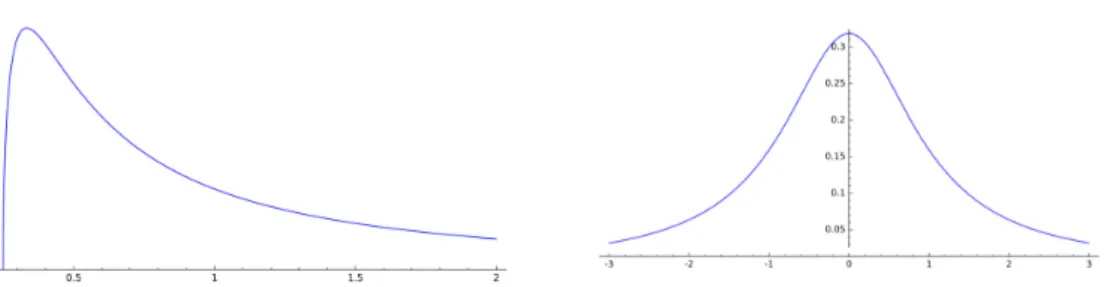
(24) Thèse de Min Wang, Université de Lille, 2019. 1.7. Stable distributions. The central limit theorem (CLT) states that the sum of a number of i.i.d. random variables with a finite variance will tend to a normal distribution as the number of variables grows. When the variance is infinite, the limit was called exceptional distributions by P. Lévy. Nowadays, we say that Definition 1.11. A random variable X is stable iff it can be obtained as 1 d (Y1 + Y2 + ⋯ + Yn − an ) Ð→ X, bn. n → ∞,. (1.14). with Y1 , Y2 , ⋯ i.i.d., an ∈ R and bn > 0.. √ If Var[Y1 ] = σ 2 < ∞, let an = nE[Y1 ], bn = nσ 2 , the CLT shows that normal distributions are all stable. Two equivalent definitions are formulated as follows. Definition 1.12. A random variable X is stable iff for any n ≥ 2, there exist a positive number cn and a real number dn such that d. X1 + X2 + ⋯ + Xn = c n X + d n d. d. (1.15). d. where X1 = X2 = ⋯ = X and independent. If dn ≡ 0, we say that X is strictly stable. Definition 1.13. A random variable X is stable iff for any positive numbers a and b, there exist a positive number c and a real number d such that d. aX1 + bX2 = cX + d d. (1.16). d. where X1 = X2 = X and independent. Starting from the definition, we can get an expression of the characteristic functions, then using the formula of Fourier transform, we can get an expression of the density by the parameter of similarity α and the parameter of positivity ρ. Since a density is always non-negative, we can obtain an admissible domain of the parameters: (α, ρ) ∈ D ∶= {α ∈ (0, 1], ρ ∈ [0, 1]} ∪ {α ∈ (1, 2], ρ ∈ [1 − 1/α, 1/α]} ρ. admissible domain of (α, ρ). 6. 1 1/α. 1 − 1/α -. 0. 1. 2. α. For (α, ρ) ∈ D, we will denote by Zα,ρ an R-random variable having strictly α-stable distribution µα,ρ , and set fα,ρ for its density, we will use the shorter notations Zα = Zα,1 and fα = fα,1 . Zα,ρ is characterized by its charcteristic function E [eitZα,ρ ] = exp [−∣t∣α eiπsgn(t)( 2 −αρ) ] , ∀ (α, ρ) ∈ D, α. (1.17). 14 © 2019 Tous droits réservés.. lilliad.univ-lille.fr.

(25) Thèse de Min Wang, Université de Lille, 2019. from which, we have d. Zα,ρ = −Zα,1−ρ ,. ∀ (α, ρ) ∈ D,. and we have necessarily cn = n1/α in (1.15). and. cα = aα + bα in (1.16). for some α ∈ (0, 2]. Another useful characterization is the Mellin transform, which is of the form E[Z−s α,ρ 1{Zα,ρ >0} ] =. Γ(1 − s) sin(πρs)Γ(s/α), απ. s ∈ (−α, 1).. (1.18). Letting s → 0, we obtain that P[Zα,ρ ≥ 0] = ρ,. ∀ (α, ρ) ∈ D,. that is why we call ρ the parameter of positivity. Observe that when ρ = 1/2, we have d Zα,1/2 = −Zα,1/2 , which means Zα,1/2 is symmetric for every α ∈ (0, 2]. The density fα,ρ has an explicit function in three specific situations only, which are: • f2,1/2 (x) =. 2. x √1 e− 2 2π. for x ∈ R, (standard gaussian density),. • f1/2 (x) =. 1 √1 e− 4x 2 πx3. • f1,ρ (x) =. sin(πρ) for x ∈ R, (standard Cauchy density with drift). π(x2 + 2 cos(πρ)x + 1). for x ≥ 0, (inverse Gamma density),. For general case, we have a convergent series representation, ∀α ∈ (0, 1], ρ ∈ [0, 1], ∀x > 0, fα,ρ (x) =. 1 Γ(1 + αn) sin(nπαρ)x−αn−1 ; ∑ (−1)n−1 π n≥1 n!. (1.19). and ∀α ∈ (1, 2], ρ ∈ [1 − 1/α, 1/α], ∀x > 0, fα,ρ (x) = x−1−α f 1 ,αρ (x−α ). α. The relation in the last formula is the so-called duality law, it is equivalent to d Z+α,ρ =. +. (Z 1 ,αρ ) α. 1 −α. ,. ∀ α ∈ (1, 2], ρ ∈ [1 − 1/α, 1/α],. (1.20). where X+ is the cutoff of X, i.e. the positive random variable with distribution function FX+ (x) = P (X ≤ x∣X ≥ 0),. x ≥ 0.. For β ∈ [−1, 1], we will denote by Sβ ( β ≠ 0 ) the 1-stable random variable having the density gβ defined in (A.23), and denote S0 the cauchy distribuiton with c0 = π2 , and c1 = 0 . The characteristic function of Sβ is of the form π E [eitSβ ] = exp (− ∣t∣ − iβt log ∣t∣) . 2 15 © 2019 Tous droits réservés.. lilliad.univ-lille.fr.

(26) Thèse de Min Wang, Université de Lille, 2019. Definition 1.14. We say that two random variables X, Y are equivalent if there exist d a > 0, b ∈ R such that: X = aY + b, and we denote by X ∼ Y. Every α-stable random variable with α ≠ 1 is equivalent to some Zα,ρ . But this is not the case for non-strictly 1-stable random variables, i.e. a non-strictly 1-stable random variable is never equivalent to a strictly stable one. The proofs of all results in this section are given in Appendix A.. 1.7.A. Lévy-Khintchine representations of stable distributions. We need the Lemma 14.11 in Sato [79] which is formulated as follows, Lemma 1.1. ∞ α ix −iπα/2 , ∫0 (e − 1) Γ(1 − α)x1+α dx = −e ∞. α −iπα/2 ix , ∫0 (e − 1 − ix) Γ(1 − α)x1+α dx = −e. for 0 < α < 1, for 1 < α < 2,. (1.22). for z > 0 with. (1.23). ∞ dx πz ixz ∫0 (e − 1 − ixz1(0,1] (x)) x2 = − 2 − iz log z + icz,. c=∫. 1. ∞. x−2 sin xdx + ∫. 1 0. (1.21). x−2 (sin x − x)dx.. Theorem 1.18. (i)For α ∈ (0, 1), ρ ∈ [0, 1], E [eitZα,ρ ] = exp (∫. ∞ −∞. (eitx − 1)ν(dx)). where. ⎧ α ⎪ ⎪c1 Γ(1−α)x1+α dx , if x > 0; ν(dx) = ⎨ α ⎪ ⎪ ⎩c2 Γ(1−α)∣x∣1+α dx, if x < 0. with c1 = sin(παρ)/ sin(πα) and c2 = sin(πα(1 − ρ))/ sin(πα). (ii) For α ∈ (1, 2), ρ ∈ [1 − 1/α, 1/α], E [eitZα,ρ ] = exp (∫. ∞ −∞. (1.24). (eitx − 1 − itx)ν(dx)). where. ⎧ α ⎪ ⎪c1 Γ(1−α)x1+α dx , if x > 0; ν(dx) = ⎨ α ⎪ ⎪ ⎩c2 Γ(1−α)∣x∣1+α dx, if x < 0. with c1 = sin(παρ)/ sin(π(2 − α)) and c2 = sin(πα(1 − ρ))/ sin(π(2 − α)). (iii)For β ∈ [−1, 1], E [eitSβ ] = exp (iat + ∫. ∞. −∞. where a ∈ R and. (1.25). (eitx − 1 − ixt1[−1,1] (x))ν(dx)) ,. ⎧ ⎪ ⎪c1 x−2 dx , if x > 0, ν(dx) = ⎨ −2 ⎪ ⎪ ⎩c2 ∣x∣ dx, if x < 0,. (1.26). 16 © 2019 Tous droits réservés.. lilliad.univ-lille.fr.

(27) Thèse de Min Wang, Université de Lille, 2019. 1−β with c1 = 1+β 2 , c2 = 2 . (iv) For ρ ∈ [0, 1],. E [eitZ1,ρ ] = exp (i˜ at + ∫ where a ˜ ∈ R and ν(dx) =. ∞ −∞. (eitx − 1 − ixt1[−1,1] (x))ν(dx)) ,. (1.27). sin(πρ) πx2 1x≠0 dx.. Proof. The proof of (i), (ii) and (iii) are similar, we first derive the representations from the above lemma for the extreme cases, i.e. {α ∈ (0, 1), ρ = ±1}, {α ∈ (1, 2), ρ = α1 or 1 − α1 } and {α = 1, β = ±1}. Then we can obtain the other cases by a simple linear combination. We do only (i) here. From (1.21), we have E [eitZα ] = exp(−e−iπsgn(t)α/2 ∣t∣α ) = exp(∫ E [eitZα,0 ] = exp(−eiπsgn(t)α/2 ∣t∣α ) = exp(∫. ∞ 0 0. −∞. (eitx − 1). (eitx − 1). α dx), Γ(1 − α)x1+α. α dx). Γ(1 − α)∣x∣1+α. For θ ∈ (−α/2, α/2), there exist c1 > 0, c2 > 0, such that eiπθ = c1 e−iπα/2 + c2 eiπα/2 , then eiπ(θ+α/2) = c1 +c2 eiπα , c2 = sin(π(α/2+θ))/ sin(πα), similarly, c1 = sin(π(α/2−θ))/ sin(πα). Substitute θ by α2 − αρ, we obtain (i). (iv) is a consequence of (iii), since Z1,ρ with ρ ∈ (0, 1) is equivalent to S0 . Note that Z1,1 ≡ 1 and Z1,0 ≡ −1. ◻ Remark 1.1. (a) From the Lévy-Khintchine representation we see that ∀ α ∈ (0, 1), ρ ∈ [0, 1], d 1/α 1/α ˜ Zα,ρ = c1 Zα − c2 Z α and ∀ α ∈ (1, 2), ρ ∈ [1 − 1/α, 1/α], d 1/α 1/α ˜ Zα,ρ = c1 Zα, 1 − c2 Z α, 1 , α. α. ˜ α,ρ is an independent copie of Zα,ρ , c1 and c2 are the same as those in the above where Z theorem. (b) For β ∈ [−1, 1], 1−β˜ d d 1+β S1 − S1 , Sβ = −S−β and Sβ = 2 2 ˜ 1 is an independent copie of S1 . where S. 1.7.B. Asymptotic expansions for the positive stable densities. Recall that the density fα of Zα is gα,−α/2 which has been studied in section A.1.B, fα (x) = The function. α x1+α. φ(−α, 1 − α; −x−α ) =. Mα (z) ∶= φ(−α, 1 − α; −z),. α x1+α. Mα (x−α ).. (1.28). 0 < α < 1,. 17 © 2019 Tous droits réservés.. lilliad.univ-lille.fr.

(28) Thèse de Min Wang, Université de Lille, 2019. is the so-called M-Wright function which has been considered in details in [63, 64]. Mainardi and Tomirotti [63] have shown that for α = 1/q, where q ≥ 2 is a positive integer, the M-Wright function can be expressed as a sum of simpler (q − 1) entire functions. In the particular case q = 2 and q = 3, they obtained 1 M 1 (z) = √ exp(−z 2 /4), 2 π and. M 1 (z) = 32/3 Ai(z/31/3 ), 3. where Ai denotes the Airy function: Ai(x) =. b 1 ∞ t3 1 t3 cos ( + xt) dt ≡ lim cos ( + xt) dt. π ∫0 3 π b→∞ ∫0 3. Thus f 1 and f 1 can be expressed as 2. 3. 1 1 f 1 (x) = √ exp(− ), x > 0, 2 3 4x 2 πx. and f 1 (x) = (3x4 )− 3 Ai((3x)− 3 ), x > 0. 1. 1. 3. They also gave their asymptotic representation for large ∣z∣ using the saddle point method, Mα (z) ∼ √. 1 2π(1 − α). (αz). α−1/2 1−α. exp (−. 1−α 1 (αz) 1−α ) , α. as ∣z∣ → +∞.. (1.29). Therefore we have the following propositions. Proposition 1.4. ∀ α ∈ (0, 1), one has fα (x) ∼. α Γ(1 − α)x1+α. as x → +∞. fα (x) ∼ cα x− 2−2α e−(1−α)(x/α) 2−α. and. with. α − 1−α. as x → 0+,. 1. cα = √. α 2(1−α) 2π(1 − α). ⋅. Remark 1.2. This proposition is a special case of proposition 2.1. Their relation is that 1 f1−α (x) = cf1,α (cx) with c = (1 − α) α−1 .. 1.7.C. Kanter’s factorization. The formula (4.5) in [64] stated that ∫0. ∞. xs Mα (x)dx =. which implies that E[Zsα ] =. Γ(s + 1) , Γ(αs + 1). Γ(1 − s/α) , Γ(1 − s). s > −1, α ∈ (0, 1),. for s < α.. Kanter [51, Corollary 4.1] found an independent factorization of the positive stable distributions d Zα = L1−1/α × Kα , (1.30) 18 © 2019 Tous droits réservés.. lilliad.univ-lille.fr.

(29) Thèse de Min Wang, Université de Lille, 2019. where L has unit exponential distribution and Kα is the so-called Kanter random variable having fractional moments E[Ksα ] =. Γ(1 − s/α) , Γ(1 − (1/α − 1)s)Γ(1 − s). for s < α,. (1.31). and in particular has a support [bα , +∞) which is bounded away from zero, with −1 1− α 1/n b−1 = lim E[K−n , α = α (1 − α) α ] 1. n→+∞. by Stirling’s formula (B.5). Several analytical properties of the density of Kα have been obtained in [50, 82]. In particular, Corollary 3.2 in [50] shows that Proposition 1.5. For every s > 0, there exists cα,s > 0 such that Ksα − cα,s is a mixture of exponential distribution. Particularly, the density of Kα − bα is CM. We will use this fact repeatedly in the chapter 3.. 1.7.D. HCM property of positive stable distributions. Pierre Bosch and Thomas Simon [23] proved that The density fα is HCM if and only if α ≤ 1/2. This result was conjectured in 1977 by Bondesson. The only if part is easy to establish because the random variable Z−1 α is not infinitely divisible, and hence cannot have a HCM density by (1.13), when α > 1/2. The if part is based on the following three lemmas. Lemma 1.2. The density of the product Γc × Ba1 ,b1 × ⋯ × Ban ,bn is HCM for every n ≥ 1, ai , bi > 0 and c < min{ai }. Lemma 1.3. For every α ∈ (0, 1), one has the a.s. convergent factorization γ(1−α Z−1 α =e d. −1 ). ∞. × ∏ an Bα+nα,1−α n=0. where γ is the Euler’s constant, and an =. eψ(1+nα)−ψ(α+nα) ,. ψ is the digamma function.. Lemma 1.4. For every a, b > 0, one has the a.s. convergent factorization ∞. d. Γa = eψ(a) × ∏ bn Ba+nb,b n=0. with bn =. eψ(a+b+nb)−ψ(a+nb) .. Combining lemmas 1.3 and 1.4 with the elementary factorization d. Ba,b+c = Ba,b × Ba+b,c one has γ(1−α Z−1 α =e d. −1 )−ψ(α). ∞. × Γα × ∏ eψ(1+nα)−ψ(2α+nα) B2α+nα,1−2α . n=0. Applying lemma 1.2 and theorem 1.17 concludes the proof. We will mimic this proof to prove a similar result for generalized stable distributions in section 2.2.B. Pierre Bosch and Thomas Simon conjectured at the end of [23] that 19 © 2019 Tous droits réservés.. lilliad.univ-lille.fr.

(30) Thèse de Min Wang, Université de Lille, 2019. Conjecture 1.4. The density of Zqα is HCM if and only if α ≤. 1 2. and ∣q∣ ≥. α 1−α .. We have proved in Chapter 3 that Z− 1−α is not HCM for α < 1/5, see Remark 3.9 (b). Thus this conjecture is not true in general. α. 1.7.E. Shape of densities of stable distributions. It is known that two-sided stable densities are real analytic on R, never vanishes, and that all their derivatives tend to zero at infinity. Hence, their n-th derivative vanishes at least n times on R by Rolle’s theorem. Definition 1.15. A smooth non-negative function on some open interval I ⊂ R is said to be bell-shaped (BS) if it vanishes at both ends of I, and if #{x ∈ Supp f, f (n) (x) = 0} = n for every n ≥ 1. W. Gawronski proved in [40] that two-sided α-stable densities are bell-shaped when α = 2 or 1/n for some n = 1, 2, 3, ⋯. T. Simon proved in [83] that positive stable distributions have bell-shaped density functions. Recently, M. Kwasnicki proved in [58] that Theorem 1.19 (Corollary 1.3 in [58]). All stable distributions on R have bell-shaped density functions. Bell-shaped (BS) functions Moreover, Kwasnicki has discovered a large class of functions f that are bell-shaped, including all smooth densities of EGGCs. Theorem 1.20 (Theorem 1.1 in [58]). Suppose that f is a locally integrable function which converges to zero at ±∞, and which is decreasing near ∞ and increasing near −∞. Suppose furthermore that for ξ ∈ R/{0} the fourier transform of f satisfies ∞. L(f ; iξ) ∶= ∫ e−iξx f (x)dx −∞ = exp [−aξ 2 − ibξ + c + ∫. ∞ −∞. (. 1 1 iξ − ( − 2 ) 1R/(−1,1) (s)) ϕ(s)ds] iξ + s s s. with a ≥ 0, b, c ∈ R, and ϕ ∶ R → R is a function with the following properties: 1. for every k ∈ Z the function ϕ(s) − k changes its sign at most once, and for k = 0 this change takes place at s = 0 ∶ sϕ(s) ≥ 0; 2. we have (∫. −1 −∞. +∫. ∞ 1. ). ∣ϕ(s)∣ ds < ∞; ∣s3 ∣. 3. we have 1. ∫−1 RL(f ; iξ)dξ < ∞,. and. limξ→0 IL(f ; iξ) = 0.. If in addition f is smooth, then f is bell-shaped. We will use this theorem to prove Theorem 3.4 (d). 20 © 2019 Tous droits réservés.. lilliad.univ-lille.fr.

(31) Thèse de Min Wang, Université de Lille, 2019. Bell-shaped of order n (BSn ) densities For a given smooth density f on (0, ∞) and n ≥ 0, let us introduce the following property: one has f ∈ BSn if ♯{x > 0, f (i) (x) = 0} = i for i ≤ n, { ♯{x > 0, f (i) (x) = 0} = n for i > n. For n ≥ 0, this property was introduced in [83] under the less natural denomination WBSn−1 - see the definition therein. Clearly, one has BS0 = CM and BS1 corresponds to whale-shaped (see Definition 3.1) functions supported on (0, +∞), which plays a role in chapter 3. Since the density of Γt has m−th derivative m m xt−1 e−x (−1)m (∑ ( ) (1 − t)p x−p ) Γ(t) p=0 p. on (0, ∞), it is an easy exercise using Rolle’s theorem and Descartes’ rule of signs to show that Γt ∈ BSn for t ∈ (n, n + 1]. In this respect, the class BSn can be thought of as an extension of the densities of Γt for t ∈ (n, n + 1]. Moreover, we have just seen that the set of densities of Γn+1 −mixtures contains the class BSn for n = 0, 1. We actually believe that this is true for all n ≥ 0. The following proposition gives us more BSn densities. Proposition 1.6 (Proposition in [83]). Let X ∈ ME∗ and λi > 0 for all i ∈ N∗ . For every n ≥ 0, the independent sum X + Exp(λ1 ) + ⋯ + Exp(λn ) has a BSn density. We will use this proposition to prove Theorem 3.4 (c).. 21 © 2019 Tous droits réservés.. lilliad.univ-lille.fr.


(33) Thèse de Min Wang, Université de Lille, 2019. Chapter 2 Density solutions to a class of integro-differential equations 2.1. Introduction and statement of the results. In this paper, we are concerned with the following integro-differential equation xm f (x) =. x 1 (x − v)α−1 f (v) dv ∫ Γ(α) 0. (2.1). on (0, ∞), with α > 0 and m ∈ R. This equation can be written in a more compact way as Iα0+ f = xm f, where Iα0+ is the left-sided Riemann-Liouville fractional integral on the half-axis. We refer to the comprehensive monograph [55] for more details on fractional operators and the corresponding differential equations. We are interested in density solutions to (2.1), that is we are searching for such f satisfying (2.1) which are also probability densities on (0, ∞). In this framework, the identities (2.1.31) and (2.1.38) in [55] imply that the auxiliary function h = Iα0+ f is a solution to the fractional differential equation Dα0+ h = x−m h,. (2.2). where Dα0+ is the left-sided Riemann-Liouville fractional derivative. This latter equation can be solved in the case m = 1 in terms of the classical Wright function - see Theorem 5.10 in [55], and we will briefly come back to this example in Section 3. Observe that density solutions to (2.1) may not exist. If α = m for example, then (2.1) becomes 1 1 (1 − v)α−1 f (xv) dv, f (x) = ∫ Γ(α) 0 and the integral of the right-hand side over (0, +∞) is infinite while the integral of the left-hand side is 1 if f is a density function. In this respect, let us also notice that the arbitrary constant Γ(α) in (2.1) was chosen without loss of generality: if fm,α is a density solution to (2.1), then fc,m,α (x) = cfm,α (cx) is for every c > 0 a density solution to xm f (x) =. x cα−m (x − v)α−1 f (v)dv. Γ(α) ∫0. 23 © 2019 Tous droits réservés.. lilliad.univ-lille.fr.

(34) Thèse de Min Wang, Université de Lille, 2019. Let us start with a few examples. When α = n is a positive integer, then (2.1) becomes an ODE of order n satisfied by the n−th cumulative distribution function Fn (x) = ∫ 0<x which is. 1 <...<xn <x. f (x1 ) dx1 . . . dxn , (n). Fn = xm Fn .. • For α = 1, we solve F1 = xm F1′ with F1 bounded and vanishing at zero. This implies x1−m. that F1′ is a density iff m > 1 with F1 (x) = e− (m−1) , that is fm,1 = F1′ is the density of 1 the Fréchet random variable ((m−1)Γ1 ) 1−m where, here and throughout, Γt denotes a Gamma random variable of parameter t > 0, with density fΓt (x) =. xt−1 e−x , Γ(t). x > 0.. • For α = 2, we solve F2 = xm F2′′ with F2 having linear growth at infinity and vanishing at zero. Supposing m > 2 and making the substitution K(x) = xν F2 ((x/2ν)−2ν ) with ν = 1/(m − 2), we obtain Bessel’s modified differential equation x2 K ′′ + xK ′ − (x2 + ν 2 )K = 0, whose solutions satisfying the required properties for F2 are constant multiples of the Macdonald function Kν . A density solution to (2.1) is then fm,2 (x) = F2′′ (x) = x−m F2 (x) = cν x−3/2−1/ν Kν (2νx−1/2ν ), where cν is the normalizing constant. On the other hand, a computation using e.g. the formula 7.12(23) p.82 in [34] shows that the independent product Γ1 × Γν+1 has density ν √ 2x2 Kν (2 x) 1(0,∞) (x). Γ(ν + 1) √ 2 By a change of variable, this implies that fm,2 is the density of ((m−2) Γ1 × Γν+1 ) 2−m . For α ≥ 3, the resulting ODE’s have higher order and do not seem to exhibit any classical special function. In section 3, however, we will see that the density solutions to (2.1) can be characterized in terms of the Gamma distribution for all integer values of α. When α is not a positive integer (2.1) is a true integro-differential equation, which can be handled via the Laplace transform L(λ) = ∫ 0. ∞. e−λx f (x) dx.. In particular, when m = n is a positive integer, the latter satisfies an ODE of order n analogous to the above, which is L = (−1)n λα L(n) . 24 © 2019 Tous droits réservés.. lilliad.univ-lille.fr.

(35) Thèse de Min Wang, Université de Lille, 2019. • For m = 1, we solve L = −λα L′ with L a completely monotone (CM) function satisfying L(0) = 1. This implies that there is a density solution to (2.1) iff α ∈ λ1−α. (0, 1) with L(λ) = e− (1−α) , that is f1,α is the density of (1 − α) α−1 Z1−α where, here and throughout, Zβ is the standard positive β-stable random variable with Laplace transform β E[e−λZβ ] = e−λ , λ ≥ 0. (2.3) 1. • For m = 2, we solve L = λα L′′ with the same restrictions on L. Supposing α < 2 and setting ν = 1/(2 − α), the same reasoning as above leads to 2ν ν √ 1 2 1 −1 L(λ) = λ Kν (2νλ 2ν ) = E[e−ν λ ν Γν ], Γ(ν) where the second equality follows again from the formula 7.12(23) p.82 in [34]. For 1 α = 1 = ν, we recover the above Fréchet density f2,1 (x) = x−2 e− x . For α ∈ (1, 2), it follows from (2.3) that f2,α is the density of the independent product ν 2ν Γ−ν ν × Z ν1 . For α ∈ (0, 1), it is not clear from classical integral formulæ on the Macdonald function that the above L is indeed a CM function viz. f2,α is a density. In Section 3, we will see that f2,α is for all α ∈ (0, 2) the density of a certain random variable involving two independent copies of Z1− α2 . The study of density solutions to (2.1) for m a positive integer was initiated in [81] and then pursued in [74], where the corresponding random variables are called "generalized stable". Apart from the classical stable case m = 1, these random variables are of interest in the case {m = 2, α ∈ (0, 1)} which is especially investigated in Section 3 of [81] and Section 7 of [74], because of its connections to particle transport along the one-dimensional lattice - see [15]. The paper [81] takes the point of view of Fox functions and shows that for all m ∈ N∗ , α ∈ (0, 1) there exists a density solution to (2.1) having a convergent power series representation at infinity and a Fréchet-like behavior at zero - see (2.12) and (2.15) therein. The paper [74] takes the point of view of size-biasing and shows that for all m ∈ N∗ , α ∈ (0, m) there exists a unique density solution to (2.1), whose corresponding random variable can be represented in the case α ∈ (m − 1, m) as a finite independent product involving the random variables Zβ and Γt - see Theorems 4.3 and 4.2 therein. In this paper, we characterize the existence and unicity of density solutions to (2.1) for all m ∈ R and α > 0, and we obtain a representation of the corresponding random variables as two infinite products involving the Beta random variable Ba,b , whose density is recalled to be fBa,b (x) =. Γ(a + b) a−1 x (1 − x)b−1 , Γ(a)Γ(b). x ∈ (0, 1).. Here and throughout, all infinite products are assumed to be independent and a.s. convergent. Our main result reads as follows. Theorem 2.1. The equation (2.1) has a density solution if and only if m > α. This solution is unique, and it is the density of −1. d. Xm,α = (a. m−a a. − a1. m ∞ m + an Γ(m) ∞ m + n d Γ( ) ∏ ( ) Ba+an,m−a ) = ( ) B1+ na , ma −1 ) ∏( a n=0 a + an Γ(a) n=0 a + n. ,. with the notation a = m − α. 25 © 2019 Tous droits réservés.. lilliad.univ-lille.fr.

(36) Thèse de Min Wang, Université de Lille, 2019. The fact that the two above infinite products are actually a.s. convergent is an easy consequence of the martingale convergence theorem - see the beginning of Section 2.1 in [59] and the references therein. The proof of the above theorem relies on the Mellin transform of f, which is by (2.1) the solution to a functional equation of first order given as (2.9) below. This kind of equation has often been encountered in the recent literature, with various point of views - see e.g. [87, 73, 57, 75]. If f is assumed to be a density, then (2.1) or (2.9) amount to a random contraction equation d Y = Bm−α,α × Yˆm−α. (2.4). connecting a random variable Y and its size-bias Yˆm−α , with the notations of the beginning of Section 2 in [74]. Our two product representations are then essentially a consequence of Theorem 3.5 in [73] and Lemma 3.2 in [74]. However, these simple representations do not seem to have been observed as yet, see in this respect the bottom of p.208 in [74]. Throughout, motivated by precise asymptotics analogous to (2.15) in [81], we will also connect the Mellin transform of the solution to (2.4) to the double Gamma function G(z; τ ), z, τ > 0. This function, also known as the Barnes function for τ = 1, was introduced in [8] as a generalization of the Gamma function. It fulfils the functional equations G(z + 1; τ ) = Γ(zτ −1 )G(z; τ ). G(z + τ ; τ ) = (2π). and. τ −1 2. τ 2 −z Γ(z)G(z; τ ) (2.5) 1. with normalization G(1; τ ) = 1. The link between these two functional equations and that of (2.9) was thoroughly investigated in [57] in the framework of Lévy perpetuities - see Section 3 therein. The normalization also implies τ −1. (2π) 2 G(τ ; τ ) = √ τ. (2.6). for every τ > 0, which will be used henceforth. A consequence of our main result is the solution to open problems related to the infinite divisibility of the density solutions to (2.1), recently formulated in [74]. Recall that the law of a positive random variable X is called a generalized Gamma convolution (X ∈ GGC for short) iff its log-Laplace exponent reads ∞ ∞ dx = aλ + ∫ log(1 + λu−1 )µ(du) − log E[e−λX ] = aλ + ∫ (1 − e−λx )k(x) x 0 0 with a ≥ 0 and ∞ k(x) = ∫ e−xu µ(du). (2.7). 0. is a CM function, whose Bernstein measure µ is called the Thorin measure of X. We now suppose m > α and denote by Xm,α the positive random variable whose density fm,α is the unique density solution to (2.1). The law of Xm,α will be denoted by Gst(m, α) −1 and called generalized stable with parameters m and α, whereas the law of Ym,α = Xm,α will be denoted by rGst(m, α), in accordance with the terminology of [74]. Observe from (2.1) that the density gm,α (x) = x−2 fm,α (x−1 ) of Ym,α is such that hm,α (x) = x1−α gm,α (x) is a positive solution to Iα− h = x2α−m h, where Iα− is the right-sided Riemann-Liouville fractional integral on the half-axis. This dual equation to (2.1) is the one appearing in a physical context for m = 2 - see (27) in [15]. 26 © 2019 Tous droits réservés.. lilliad.univ-lille.fr.

(37) Thèse de Min Wang, Université de Lille, 2019. Corollary 2.1. With the above notations, one has: (a) Xm,α ∈ GGC for all m > α. (b) Xm,α ∈ HCM ⇔ Ym,α ∈ ID ⇔ m ≤ 2α. Part (a) of the corollary is a generalization of Theorem 5.3 in [74], solving the open questions formulated thereafter. Besides, by e.g. Theorem III.4.10 in [84], it shows that the density solution fm,α to (2.1) is also the unique density solution to x. xf (x) = ∫ km,α (x − y) f (y) dy 0. (2.8). where km,α is the CM function associated to Xm,α through (2.7). This latter equation is known as Steutel’s integro-differential equation for infinitely divisible densities. Except in the obvious case m = 1, the link between the two convolution kernels (x − y)α−1 and km,α (x − y) is mysterious, and the function km,α is not explicit in general. See however Section 3 for an analytical treatment of km,α in the cases m = 2α and m = 2. Part (b) gives a characterization of the infinite divisibility of the law rGst(m, α), and it is an extension of Theorem 5.1 in [74]. It can also be viewed as a generalization of the main result of [23], which handles the case m = 1. As will be observed in Remark 2.1 (a) below, its proof also allows us to solve entirely the open question stated after Theorem 3.2 in [74]. We now turn to the asymptotic behavior of the densities fm,α at zero and infinity. This is a basic question for the classical special functions, which is investigated e.g. all along [34]. When m is an integer, the densities fm,α are Fox functions and in [81], the general results of [24] are used in order to derive convergent power series representations at infinity, with an exact first order polynomial term, as well as a non-trivial exponentially small behavior at zero - see (2.20) and (2.21) therein. In general, fm,α is not a Fox function. Indeed, following from (2.10) (B.6) and (B.7), fm,α is a Fox function iff there exist a1 , ⋯, aM , c1 , ⋯, cN ≥ 0 and b1 , ⋯, bM , d1 , ⋯, dN > 0 such that M N z ai z ci 1 − zα = − , ∑ ∑ (1 − z)(1 − z m−α ) i=1 1 − z bi i=1 1 − z di. ∀ z ∈ (0, 1).. m The answer is positive if α ∈ N, if m ∈ N, or if m−α ∈ N, which will be studied in section 2.3.A. But it is not always right, for example, α = 1/2, m = 3/2. However, we can show the following estimates, which generalize (2.20) and (2.21) in [81].. Proposition 2.1. With the above notation, one has fm,α (x) ∼. xα−m−1 Γ(α). as x → ∞. and. fm,α (x) ∼ cm,α x−. with m−2. cm,α. m(1+α) 2α. e−( m−α )x α. α−m α. as x → 0,. α(1−m). (2π) 2 (m − α) 2(m−α) √ = ⋅ α G(m, m − α). The estimate at infinity is an elementary consequence of (2.1). The derivation of the estimate at zero, much more delicate, is centered around the exact case m = 2α which corresponds to the Fréchet random variable Γ−1 α . When m > 2α, the underlying random variable is the exponential functional of a Lévy process without negative jumps, and we can apply the recent Tauberian results of [75]. To handle the case m < 2α which has 27 © 2019 Tous droits réservés.. lilliad.univ-lille.fr.