Decentralized Prediction of End-to-End Network Performance Classes

(1)

Decentralized Prediction of End-to-End

Network Performance Classes

Yongjun Liao

*

_{, Wei Du}

†

_{, Pierre Geurts}

‡

_{, and Guy Leduc}

* *_{Research Unit in Networking, University of Li `ege, Belgium} †_{Intelligent and Interactive Systems, University of Innsbruck, Austria}

‡_{Systems and Modeling, University of Li `ege, Belgium}

ABSTRACT

In large-scale networks, full-mesh active probing of end-to-end performance metrics is infeasible. Measuring a small set of pairs and predicting the others is more scalable. Un-der this framework, we formulate the prediction problem as matrix completion, whereby unknown entries of an incom-plete matrix of pairwise measurements are to be predicted. This problem can be solved by matrix factorization because performance matrices have a low rank, thanks to the corre-lations among measurements. Moreover, its resolution can be fully decentralized without actually building matrices nor relying on special landmarks or central servers.

In this paper we demonstrate that this approach is also applicable when the performance values are not measured exactly, but are only known to belong to one among some predefined performance classes, such as "good" and "bad". Such classification-based formulation not only fulfills the re-quirements of many Internet applications but also reduces the measurement cost and enables a unified treatment of var-ious performance metrics. We propose a decentralized ap-proach based on Stochastic Gradient Descent to solve this class-based matrix completion problem. Experiments on var-ious datasets, relative to two kinds of metrics, show the accu-racy of the approach, its robustness against erroneous mea-surements and its usability on peer selection.

Categories and Subject Descriptors

C.2.4 [Computer Communication Networks]: Dis-tributed Systems—DisDis-tributed Applications

General Terms

Measurement

Permission to make digital or hard copies of all or part of this work for personal or classroom use is granted without fee provided that copies are not made or distributed for profit or commercial advantage and that copies bear this notice and the full citation on the first page. To copy otherwise, to republish, to post on servers or to redistribute to lists, requires prior specific permission and/or a fee.

Keywords

network performance classification, matrix completion, matrix factorization, stochastic gradient descent

1. INTRODUCTION

The knowledge of end-to-end network performance is essential for Internet applications to achieve Qual-ity of Service (QoS) objectives [24, 17, 18, 27]. Typi-cal QoS objectives relate to performance metrics such as network delay, often represented by round-trip time (RTT), available bandwidth (ABW) and packet loss rate (PLR) [6]. Under a chosen metric, the acquisition of end-to-end network performance amounts to perceiv-ing measurements of some kind, commonly in the form of real-valued quantities.

While such quantitative measures have been widely accepted by the networking community, qualitative mea-sures of whether the performance of a network path is good enough already carry information of great inter-est from the application point of view. For instance, streaming media applications care more about whether the ABW of a path is high enough to provide smooth playback quality. In peer-to-peer applications, although finding the nearest nodes to communicate with is prefer-able, it is often enough to access a nearby node with a limited loss compared to the nearest node. Moreover, qualitative measures have two nice properties. First, they are generally coarse and can therefore be acquired with cheaper means. The cost reduction is more signif-icant for metrics such as the ABW whose measurement is expensive. Second, qualitative measures are stable and better reflect long-term characteristics of network paths, which means that they can be probed less often. In this paper, we consider the inference of whether the performance of a network path is good enough as a bi-nary classification problem [2] that classifies the perfor-mance, according to a metric, into one of the two classes of “good” and “bad”1_{. Such class-based representation}

1

Depending on the context, the class labels of “good” and “bad” may refer to “well-performing” and “poorly-performing” or “well-connected” and “poorly-connected”.

(2)

enables a unified and equal treatment of different met-rics such as RTT and ABW, which have vastly distinct characteristics and are usually discriminatively treated. A major obstacle to the utilization of end-to-end net-work performance by Internet applications is the scal-able acquisition in large-scale networks. As full-mesh active probing among all nodes is obviously infeasible, a natural idea is to probe a small set of pairs and then pre-dict the performance between other pairs where there are no direct measurements, which has been successfully used to estimate RTTs in various Network Coordinate Systems (NCS) [8].

Under this “probe a few and predict many” frame-work, we investigate the prediction of end-to-end net-work performance classes in large-scale netnet-works. In contrast to previous work, the prediction of network performance is formulated as a matrix completion prob-lem where a partially observed matrix is to be com-pleted [5]. Here, the matrix contains binary perfor-mance measures between network nodes with some of them known and the others unknown, and thus to be filled. Matrix completion is only possible if matrix en-tries are largely correlated, which holds for many met-rics in the Internet because Internet paths with nearby end nodes often overlap and share common bottleneck links. These redundancies among network paths cause the constructed performance matrix to be low rank (we will demonstrate this empirically for RTT and ABW).

The low-rank nature of various performance matrices enables their completion by matrix factorization tech-niques. This paper presents a novel decentralized ma-trix factorization approach based on Stochastic Gradi-ent DescGradi-ent (SGD). By letting network nodes exchange messages with each other, the factorization is collab-oratively and iteratively performed at all nodes with each node equally retrieving a small number of mea-surements. A distinct feature of our approach is that it is fully decentralized, with neither explicit construc-tion of matrices nor special nodes such as landmarks or a central node where measurements are collected and processed. Extensive experiments on various RTT and ABW datasets show that our approach is simple, suit-able for dealing with dynamic measurements in large-scale networks and robust against large amount of erro-neous measurements. Furthermore, we demonstrate the benefits of our binary classification approach on peer selection, a problem at the heart of many Internet ap-plications. These experiments highlight not only the accuracy and the applicability of our approach but also its advantage in terms of measurement cost reduction.

The rest of the paper is organized as follows. Sec-tion 2 describes related work. SecSec-tion 3 introduces the metrics and the classification of end-to-end network performance. Section 4 gives the formulation of net-work performance prediction as matrix completion and

its resolution by low-rank matrix factorization. Sec-tion 5 describes the decentralized matrix factorizaSec-tion algorithms based on Stochastic Gradient Descent. Sec-tions 6 experiments our approach on three publicly avail-able datasets of RTT and of ABW. Conclusions and future work are given in Section 7.

2. RELATED WORK

Most related work on network performance prediction focused on the prediction of real values of some perfor-mance metric with a particular interest for the RTT. Examples include Global Network Positioning [14], Vi-valdi [7], Internet Distance Estimation Service [13] and Decentralized Matrix Factorization [12]. The predic-tion of ABW is less successful with SEQUOIA the only work found in the literature that embedded ABW mea-surements into a tree metric [16]. On predicting perfor-mance classes, [20] is to our knowledge the only related work that used an advanced machine learning tech-nique, namely max-margin matrix factorization (MMMF) [22]. Although successful especially thanks to the incor-poration of active sampling, MMMF required a semi-definite programming solver that only works for small-scale problems and in a centralized manner.

The main contributions of our work are the treatment of network performance as classes, instead of real values, and the formulation of the class prediction problem as matrix completion. Although numerous approaches to matrix completion have been proposed, few of them are designed for network applications where decentralized processing of data is appreciated. Thus, we developed a fully decentralized approach based on Stochastic Gra-dient Descent (SGD) which is founded on the stochastic optimization theory with nice convergence guarantees [3]. Two slightly different algorithms are proposed for dealing with RTT and with ABW due to their different measurement methodology. We then studied empiri-cally the sensitivity of the algorithms to the parameters, its robustness against erroneous measurements and its applicability in Internet applications.

3. METRICS AND CLASSIFICATION OF

NETWORK PERFORMANCE

3.1 Metrics of Network Performance

While ultimately the performance of a network path should be judged by the QoS perceived by end users, it is important to define an objective metric that is di-rectly measurable without users’ interventions. Among the commonly-used metrics mentioned earlier, this pa-per only discusses RTT and ABW due to the availability of the data and the relatively rare occurrence of packets losses in the Internet [6].

(3)

The RTT is one of the oldest and most commonly-used network measurements due partially to its ease of acquisition by using ping with little measurement over-head, i.e., few ICMP echo request and response packets between the sender and the target node. Although the one-way forward and reverse delays are not exactly the same due to e.g. the routing policy and the Internet in-frastructure, the RTTs between two network nodes can approximately be treated as symmetric.

3.1.2 Available Bandwidth (ABW)

The ABW is the available bandwidth of the bottle-neck link on a path. A comparative study has shown that tools based on self-induced congestion are generally more accurate [21]. The idea is that if the probing rate exceeds the available bandwidth over the path, then the probe packets become queued at some router, resulting in an increased transfer time. The ABW can then be es-timated as the minimum probing rate that creates con-gestions or queuing delays. To this end, pathload [10] sends trains of UDP packets at a constant rate and ad-justs the rate from train to train until congestions are observed at the target node. Pathchirp [19] reduces the probe traffic by varying the probe rate within a train exponentially.

Compared to RTT, measuring ABW is much more costly and less accurate, suffering from an underesti-mation bias due to the bursts of network traffic and the presence of multiple links with roughly the same ABW. This bias can be relieved by increasing the probe packet train length at the cost of more measurement overhead [6]. In contrast to the RTT which is inferred by the sender, the ABW is clearly asymmetric and its measurement is inferred at the target node.

3.2 Classification of Performance Metrics

The classification of network performance amounts to determining some qualitative measure that reflects how well a path can perform according to a metric. In this paper, we focus on the classification of network performance into two classes of “good” and “bad”, rep-resented by 1 and −1 respectively, independently from the actual metric used.

A straightforward approach to classifying network per-formance is by thresholding, i.e., comparing the value of the metric with a classification threshold, denoted by τ, which is determined to meet the requirements of the applications. For example, Google TV requires a broad-band speed of 2.5Mbps or more for streaming movies and 10Mbps for High Definition contents [9]. Accord-ingly, τ = 2.5Mbps or 10Mbps can be defined for ABW to separate “good” paths from “bad” ones. The impact of τ will be demonstrated in Section 6.

Classification by thresholding is directly applicable to

RTTs whose measurements are cheap. For the ABW, it is preferable to directly obtain the class measures without the explicit acquisition of the values in order to reduce measurement overhead. This is plausible for tools based on self-induced congestion as each probe by sending a UDP train at a constant rate naturally yields a binary response of “yes” or “no” that suggests whether the ABW is larger or smaller than the probe rate. Thus, the direct classification of ABW is trivial and can be done with existing tools such as pathload and pathchirp with little modification:

pathload Send UDP trains at a constant rate of τ, and classify the path as “good” if no congestion is observed and “bad” otherwise.

pathchirp Use pathchirp with fewer and shorter probe trains, and threshold by τ the rough and inaccu-rate quantities obtained.

The directly measured performance classes may be in-accurate especially for those paths with metric quanti-ties close to τ. We will demonstrate the impact of the inaccuracy of the class measures in Section 6.

The classification of other performance metrics can be done similarly by exploiting their different nature and different measurement techniques. As generally data acquisition undergoes the accuracy-versus-cost dilemma that accuracy always comes at a cost, coarse measures of performance classes are always cheaper to obtain than exact quantities, regardless of the metric used.

4. NETWORK PERFORMANCE

PREDIC-TION BY MATRIX FACTORIZAPREDIC-TION

4.1 Formulation as Matrix Completion

The problem of network performance prediction can generally be formulated as a matrix completion prob-lem. Specifically, assuming n nodes in a network, given a partially observed n × n matrix X containing perfor-mance measures in the form of either real-valued quan-tity or discrete-valued class, a matrix of the same size

ˆ

X needs to be found that best predict the unobserved entries of X. Denote xij the true performance measure

from node i to node j and ˆxij the predicted measure.

We refer to the estimation of discrete-valued classes as class-based prediction and the estimation of real-valued quantities as quantity-based prediction.

A common approach to matrix completion is low-rank approximation, which minimizes the following function

L(X, ˆX, W ) = n X i,j=1 wijl(xij, ˆxij), (1) subject to Rank( ˆX) = r n. where W is a weight matrix with wij = 1 if xij is known

(4)

1

5

10

15

20

0

0.2

0.4

0.6

0.8

1 # singular value

singular values

RTT

RTT class

ABW

ABW class

Figure 1: The singular values of a RTT and a ABW matrix and of their binary class matrices. The RTT matrix is 2255×2255 and extracted from the Meridian dataset [25]. The ABW matrix is 201 × 201 and extracted from the HP-S3 dataset [26]. The binary class matrices are obtained by thresholding their corresponding measurement matrices with τ equal to the median value of each dataset. The singular values are normalized so that the largest singular values of all matrices are equal to 1.

difference between an estimate and its desired or true value. For predicting real-valued quantities, the L2 or

square loss function is commonly used. For predicting discrete-valued classes, more often used are the hinge and the logistic loss functions [2]. These different loss functions are given below.

• L2 or square loss function: l(x, ˆx) = (x − ˆx)2;

• hinge loss function: l(x, ˆx) = max(0, 1 − xˆx); • logistic loss function: l(x, ˆx) = ln(1 + e−xˆx_).

Note that the hinge loss function is not differentiable. In the above loss functions, x is the reference value and ˆx is the predicted value. In the setting of bi-nary classification, x is either 1 or -1 and ˆx is typically real-valued and its sign usually represents the predicted class. Both the hinge and logistic loss functions are such that values of xˆx lower than 1 are strongly penalized and otherwise less or not penalized. These classification loss functions are thus not sensitive to the actual value of ˆx as long as its sign matches the sign of x. This contrasts to the L2loss function which has smaller penalties when

ˆx approaches to x.

The assumption in this low-rank approximation is that the entries of X are largely correlated, which causes X to have a low effective rank. To show that it holds for our problem, Figure 1 plots the singular values of a RTT and a ABW matrix and of their binary class matrices. It can be seen that the singular values of all matrices decrease fast, indicating strong correlations in

both RTT and ABW measurements. The low-rank na-ture of many other RTT datasets have been previously reported in [23].

4.2 Low-Rank Matrix Factorization

Directly minimizing eq. 1 is difficult due to the rank constraint. However, as ˆX is of rank r, we can factorize it into the product of two smaller matrices,

ˆ

X = UVT_, ₍₂₎

where U and V have r columns. Therefore, we can look for (U, V ) instead by minimizing

L(X,U, V, W, λ) = (3) n X i,j=1 wijl(xij, uivTj) + λ n X i=1 uiuTi + λ n X i=1 vivTi ,

where uiand viare the ith rows of U and V respectively,

and uivjT = ˆxij is the estimate of xij. λ is the

regular-ization coefficient that controls the extent of the regu-larization, the incorporation of which is to overcome a well-known problem called overfitting in the field of ma-chine learning [2]. In words, directly minimizing eq. 3 without regularization often leads to a “perfect” model with no or little errors on the training data (i.e., the known entries) while having large errors on the unseen data (i.e., the unknown entries).

The class of techniques to minimize eq. 3 is matrix factorization. In the presence of missing entries or in case of loss functions other than the L2 loss, eq. 3

be-comes non-convex and a local optimal solution can be found by iterative optimization methods such as Gra-dient Descent and Newton algorithms [4]. Note that matrix factorization has no unique solutions as

ˆ

X = UVT _{= UGG}−1_VT_, ₍₄₎

where G is any arbitrary invertible matrix. Therefore, replacing U by UG and VT _{by G}−1_VT _{will not change}

the approximation error.

4.3 System Architecture

The above low-rank matrix factorization is generic to predict network performance of all kinds, by all metrics and in the form of either quantity or class. In this paper, we focus on binary classification where xijin X is either

1 or −1, representing “good” and “bad”.

Figure 2 illustrates a unified architecture that con-sists of a measurement module and a prediction mod-ule. The measurement module probes the performance classes of a small number of paths and put them in the corresponding entries of a large matrix. The predic-tion module estimates the missing entries by applying a matrix factorization technique. The estimates of the missing entries are typically real-valued and the corre-sponding predicted classes can be determined by e.g. taking the sign of ˆxij.

(5)

-1 -1 1 1 -1 1 -1 1 1 1 -1 1 -1 1 -1 -1 1 1 -1 1 -1 -1 1 1 -1 1 -1 1 1 1 1 -1 X ≈ U z}|{ r columns × _VT = -3.4 0.6 -0.4-3.0 4.5 -1.4 2.4 -0.3 1.7 0.9 3.3 -2.5 2.1 1.3 2.5 -2.7 -3.1-1.7 2.1 1.2 -2.8 1.9 -1.6-0.9 2.3 5.5 -2.6 1.8 2.5 4.3 -6.1 3.6 2.5 2.0 -1.5 -0.3-2.7-3.6-2.1-2.6 -0.1 4.1 -2.5-1.0 0.9 4.3 -2.3 5.1 3.2 0.8 3.4 4.6 -1.4 3.6 -2.5-1.6 ˆ X -1 1 -1 -1 1 -1 1 -1 1 1 1 -1 1 1 1 -1 -1 -1 1 1 -1 1 -1 -1 1 1 -1 1 1 1 -1 1 1 1 -1 -1 -1 -1 -1 -1 -1 1 -1 -1 1 1 -1 1 1 1 1 1 -1 1 -1 -1 sign(ˆxij) Prediction Measurement Available Bandwidth i j

probe UDP train sent atτMbps

Observe congestions?

No Yes

Round Trip Time

i j

ping ICMP packets

ping ACK packets

Receive ACKs withinτms?

Yes No

Figure 2: Architecture of class-based network performance measurement and prediction. Note that the diagonal entries of X and ˆX are empty.

5. DECENTRALIZED

MATRIX FACTORIZATION BY

STOCHASTIC GRADIENT DESCENT

The above system has a centralized architecture that requires the collection and the processing of the mea-surements at a central node. This section introduces a fully decentralized matrix factorization approach based on a particular stochastic optimization method, namely Stochastic Gradient Descent (SGD).

5.1 Stochastic Gradient Descent (SGD)

SGD is one of stochastic optimization methods that has been widely used for on-line and large-scale machine learning [3]. It is a variation of traditional Batch Gradi-ent DescGradi-ent. However, instead of collecting all training samples beforehand and computing the gradients over them, each iteration of SGD chooses one training sam-ple at random and updates the parameters being esti-mated along the negative gradients computed over that chosen sample. Averaging each SGD update over all possible choices of the training samples would restore the batch gradient descent [3].

SGD is particularly suitable for solving the problem of network performance prediction, as measurements can be acquired on demand and processed locally with

no need to store them. It also has simple update rules that involve only vector operations and is able to deal with large-scale dynamic network measurements.

5.2 SGD for Network Performance Prediction

As a decentralized optimization of eq. 3 forbids the explicit constructions of any matrices, each row of U and of V , ui and vi, are stored distributively at each

node of the network. In the sequel, ui and vi will be

called the coordinates of node i. To calculate uiand vi,

i = 1, . . . , n, only local measurements related to node i are needed.

Due to their different measurement methodology, RTT and ABW are treated slightly differently.

5.2.1 SGD for Dealing with RTT

RTT is symmetric and is probed and inferred by the sender. Thus, when a RTT measurement xijis acquired

and available at node i, uiof node i can be immediately

updated by using xij. As xij = xji for RTT, xij can

also be used by node i to update vi.

Hence, given xij, the errors to be reduced at node i

are

Eij = l(xij, uivTj) + λuiuTi, (5)

Eij_{= l(x}

(6)

The gradients, by ignoring the non-differentiability of some loss functions, are given by

dEij dui = dl(xij, uivjT) dui + λui, (7) dEij dvi = dl(xij, ujviT) dvi + λvi, (8)

Note that we drop the factor of 2, from the derivatives of the regularization terms and of the L2 loss function

below, for mathematical convenience. The update rules of ui and vi are

ui= (1 − ηλ)ui− ηdl(xij, uiv T j) dui , (9) vi= (1 − ηλ)vi− ηdl(xij, ujv T i ) dvi . (10)

where η is a learning rate.

5.2.2 SGD for Dealing with ABW

Different from RTT, ABW is asymmetric and is probed by the sender but inferred by the target node. Thus, when a ABW measurement xij is available at node j,

node j needs to send xij to node i so that ui of node i

and vj of node j can both be updated by using xij.

Hence, given xij, the error to be reduced at node i

and at node j is

Eij= l(xij, uivjT) + λuiuTi + λvjvjT. (11)

With the gradients similarly defined as above, the up-date rules of ui and vj are

ui= (1 − ηλ)ui− ηdl(xij, uiv T j) dui , (12) vj= (1 − ηλ)vj− ηdl(xij, uiv T j) dvj . (13)

5.2.3 Gradients of Loss Functions

For classification, the hinge and the logistic loss func-tions are the most commonly-used and adopted here. The gradients are given below. Without causing any confusion, the subscripts are dropped.

• For the hinge loss function, the gradients2_{are zeros}

for correctly classified samples, i.e., those of 1 − xuvT _{6 0, and otherwise}

dl(x, uvT₎

du = −xv, (14)

dl(x, uvT₎

dv = −xu, (15)

2

As the hinge loss function is not differentiable, the gradient does not exist and is approximated by the subgradient [1]. However, we will only use the term gradient and gradient descent in this paper, following the convention in [3].

Algorithm 1 DMF SGD RT T (i, j)

1: node i probes node j for the RTT;

2: node j sends u_j and v_j to node i when probed; 3: node i infers x_ij when receiving the reply; 4: node i updates u_i and v_i by eqs. 9 and 10;

Algorithm 2 DMF SGD ABW (i, j)

1: node i probes node j for the ABW and sends u_i; 2: node j infers x_ij when probed;

3: node j sends x_ij and v_j to node i; 4: node j updates v_j by eq. 13;

5: node i updates u_iby eq. 12 when receiving the reply;

• For the logistic loss function, dl(x, uvT₎ du = − xv 1 + exuvT, (16) dl(x, uvT₎ dv = − xu 1 + exuvT, (17)

The gradients of the L2 loss functions for regression

are also given here, dl(x, uvT₎

du = −(x − uvT)v, (18)

dl(x, uvT₎

dv = −(x − uvT)u, (19)

as they will be used in Section 6 for the purpose of com-parison of class-based and quantity-based prediction in the application of peer selection.

5.3 Algorithms

Thus, two SGD-based decentralized matrix factoriza-tion algorithms3_{, denoted by DMFSGD, were designed}

for dealing with RTT and with ABW, given in Algo-rithm 1 and in AlgoAlgo-rithm 2. Our DMFSGD algoAlgo-rithms have the same architecture as Vivaldi [7] where each node randomly and independently chooses a neighbor set of k nodes as references and randomly probes one of its neighbors at each time. The coordinates of the nodes are initialized with random numbers uniformly distributed between 0 and 1. Empirically, the DMF-SGD algorithms are insensitive to the random initializa-tion of the coordinates as well as the random selecinitializa-tion of the neighbors.

6. EXPERIMENTS AND EVALUATIONS

In this section, we evaluate our DMFSGD algorithms and study the sensitivity to the parameters, the robust-ness against erroneous measurement and the applicabil-ity on peer selection.

3

The matlab implementation of the algorithms is available at http://www.run.montefiore.ulg.ac.be/~liao/DMFSGD.

(7)

6.1 Datasets and Evaluation Criteria

The evaluations were performed on the following pub-licly available datasets.

Harvard contains 2, 492, 546 dynamic measurements of application-level RTTs, with timestamps, be-tween 226 Azureus clients collected in 4 hours [11]. Meridian contains static RTT measurements between 2500 network nodes obtained from the Meridian project [25].

HP-S3 contains ABW measurements between 459 net-work nodes collected using the pathchirp tool [26]. As the raw dataset is highly sparse with 55% miss-ing data, we extracted 231 nodes to construct a dense ABW matrix with 4% missing entries. In the simulations, the static measurements in Meridian and HP-S3 are used in random order, whereas the dy-namic measurements in Harvard are used in time order according to the timestamps. We built a static ma-trix for Harvard by extracting the median values of the streams of measurements between each pair of nodes and used it as the ground truth.

The following evaluation criteria [2] were used. ROC A Receiver Operating Characteristic (ROC) curve

is a graphical plot of the true positive rates (TPR) versus the false positive rates (FPR) for a binary classifier as its discrimination threshold is varied. AUC The AUC is the area under the ROC curve. As

the TPR and the FPR range from 0 to 1, the max-imal possible value of AUC is 1 which means a perfect classification. In practice, AUC is smaller than 1. The closer it is to 1, the better.

Precision-Recall The precision for a class is the num-ber of true positives divided by the total numnum-ber of elements labeled as belonging to the positive class, i.e. the sum of true positives and false positives, and the recall for a class is equal to the TPR. More precisely, the ROC and Precision-Recall curves are obtained by varying a discrimination threshold τc

when deciding the classes from ˆxij’s. For a given τc, ˆxij

is turned into 1 if ˆxij> τcand into −1 otherwise. Then,

the true positive rate, false positive rate and precision for the given τc can be computed by comparing xij’s

and the binarized ˆxij’s. The ROC and Precision-Recall

curves are then obtained by varying τcfrom −∞ to +∞.

These evaluation criteria are interesting and commonly used because they show the prediction accuracies under different τc’s.

6.2 Impact of Parameters

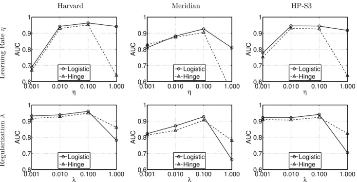
We demonstrate the impact of the parameters to the accuracy of the prediction, including learning rate η,

regularization coefficient λ, loss function l: hinge or logistic, rank r, neighbor number k and classifi-cation threshold τ.

6.2.1

η

,

λ

and

l

η controls the step of each update, which has to be small enough to guarantee the convergence of the algo-rithms while large enough to converge fast. λ trades off between the fitting errors and the norms of the so-lutions, which, similar to η, has to be small enough to guarantee the overall fitness of the factorization while large enough to avoid overfitting. Besides, the incorpo-ration of the regularization enforces the coordinates of the nodes to have low norms and helps overcome the drifts of the coordinates due to the non-uniqueness of the factorization in eq. 4.

We experimented with different configurations of η and λ under different loss functions, shown in Figure 3. It can be seen that λ = 0.1 and η = 0.1 work well for all three datasets and that the logistic loss function out-performs the hinge loss function in most cases. Thus, unless stated otherwise, λ = 0.1, η = 0.1 and the logis-tic loss function are used by default.

6.2.2

r

and

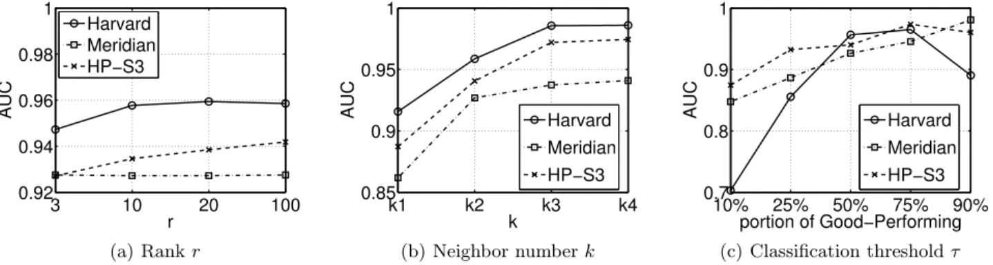
k

Intuitively, r is the number of unknown variables in each coordinate and k is the number of known data used to estimate each coordinate. Clearly, increasing k is equivalent to adding more data thus always helps improve the accuracy. However, a large k also means a higher measurement overhead which may outweigh the benefits of the accurate prediction. On the other hand, increasing r is equivalent to adding more variables to estimate, consuming more data. We found that a pair of relatively small k and r can already provide suffi-cient classification accuracy, shown in Figure 4(a) and 4(b), and further increasing k and r is either costly or worthless. Thus, unless stated otherwise, r = 10 and k = 10, 32 and 10 for Harvard, Meridian and HP-S3 respectively are used by default for all datasets.

6.2.3

τ

The classification threshold τ significantly affects the proportions of the two classes, shown in Table 1, which in turn have some impacts on the prediction accuracy, shown in Figure 4(c). Although in practice τ is de-termined according to the requirements of the applica-tions, we nevertheless set τ to the median value of each dataset by default.

6.2.4 Discussions

The default parameter configuration of λ = 0.1, η = 0.1, r = 10 and the logistic loss function is not guar-anteed to be optimal for different k’s and τ’s and on different datasets. However, fine parameter tuning is

(8)

Harvard Meridian HP-S3 Learning Rate η 0.001 0.010 0.100 1.000 0.6 0.7 0.8 0.9 1 η AUC Logistic Hinge 0.001 0.010 0.100 1.000 0.6 0.7 0.8 0.9 1 η AUC Logistic Hinge 0.001 0.010 0.100 1.000 0.6 0.7 0.8 0.9 1 η AUC Logistic Hinge Regularization λ 0.001 0.010 0.100 1.000 0.6 0.7 0.8 0.9 1 λ AUC Logistic Hinge 0.001 0.010 0.100 1.000 0.6 0.7 0.8 0.9 1 λ AUC Logistic Hinge 0.001 0.010 0.100 1.000 0.6 0.7 0.8 0.9 1 λ AUC Logistic Hinge

Figure 3: AUCs under different η’s and λ’s on different datasets. The first row shows the impact of η under λ = 0.1 and the second row shows the impact of λ under η = 0.1. r = 10 in this figure. k = 10, 32 and 10 for the Harvard, Meridian and HP-S3 datasets respectively. τ is set to the median value of each dataset, i.e. τ = 132ms for Harvard, 56ms for Meridian and 43Mbps for HP-S3.

Table 1: Impact of τ on portions of “good” paths in different datasets.

“Good”% Harvard Meridianτ HP-S3

(ms) (ms) (Mbps) 10% 27.5 19.4 88.2 25% 59.9 36.2 72.2 50% 131.6 56.4 43.1 75% 249.6 88.1 14.4 90% 324.2 155.2 10.4

difficult, if not impossible, for network applications due to the dynamics of the measurements and the decentral-ized processing where local measurements are processed locally with no central node to gather information.

Figure 5 shows that the recommended default pa-rameters produced fairly accurate results on all three datasets which are largely different from each other. The insensitivity to the parameters is probably because the inputs are binary classes and take values of either 1 or −1 regardless of the actual metric and values. The rightmost plot in Figure 5 illustrates the convergence speeds in terms of the AUC improvements with respect to the average measurement number per node, i.e. the total number of measurements used by all nodes divided

by the number of nodes4_{. It can be seen that the}

DMF-SGD algorithms converges fast after each node probes, on average, no more than 20 × k measurements from its k neighbors. Table 2 shows the accuracy rates, i.e., the percentage of the correct predictions, and the confu-sion matrices, computed by taking the sign of ˆxij’s and

then comparing with the corresponding xij’s. These

measures show intuitively the accuracy of our approach under the default parameters.

6.3 Robustness Against Erroneous Labels

This section evaluates the robustness of the DMF-SGD algorithms against erroneous class labels which arise from inaccurate measurements due to

• inaccurate measurement techniques which particu-larly affect those paths with metric quantities close to τ;

• network anomaly such as attacks from malicious nodes and sudden traffic bursts which affect every path equally.

4

For P2PSim1740 and Meridian2500, at any time, the num-ber of measurements used by each node is statistically the same for all nodes due to the random selections of the source and the target nodes in the updates. For Harvard226, this number is significantly different for different nodes because the paths were passively probed with uneven frequencies.

(9)

3 10 20 100 0.92 0.94 0.96 0.98 1 r AUC Harvard Meridian HP−S3 (a) Rank r k1 k2 k3 k4 0.85 0.9 0.95 1 k AUC Harvard Meridian HP−S3 (b) Neighbor number k 10% 25% 50% 75% 90% 0.7 0.8 0.9 1 portion of Good−Performing AUC _Harvard Meridian HP−S3 (c) Classification threshold τ

Figure 4: AUCs under different k’s, r’s and τ’s on different datasets. The left plot shows the impact of r under k = 10 for Harvard, 32 for Meridian and 10 for HP-S3. The middle plot shows the impact of k under r = 10 for all datasets. The experimented k’s are k1 = 5, k2 = 10, k3 = 30 and k4 = 50 for

both Harvard and HP-S3 and k1 = 16, k2 = 32, k3 = 64 and k4 = 128 for Meridian. τ in the left and

middle plots is set to the median value of each dataset. The right plot shows the impact of τ under r = 10 for all datasets and k = 10 for Harvard, 32 for Meridian and 10 for HP-S3. The experimented τ’s for different datasets are listed in Table 1 to generate different portions of “good” paths.

0 0.1 0.2 0.3 0.4 0.5 0.5 0.6 0.7 0.8 0.9 1 FPR TPR Harvard Meridian HP−S3 (a) ROC 0 0.2 0.4 0.6 0.8 1 0.5 0.6 0.7 0.8 0.9 1 recall precision Harvard Meridian HP−S3 (b) Precision-Recall 0 10 20 30 40 50 0.8 0.85 0.9 0.95 1 measurement number (× k) AUC Harvard Meridian HP−S3 (c) AUC

Figure 5: The accuracy of class-based prediction by DMFSGD on different datasets under the default parameter configuration. The rightmost plot shows the AUC improvements with respect to the average measurement number used by each node.

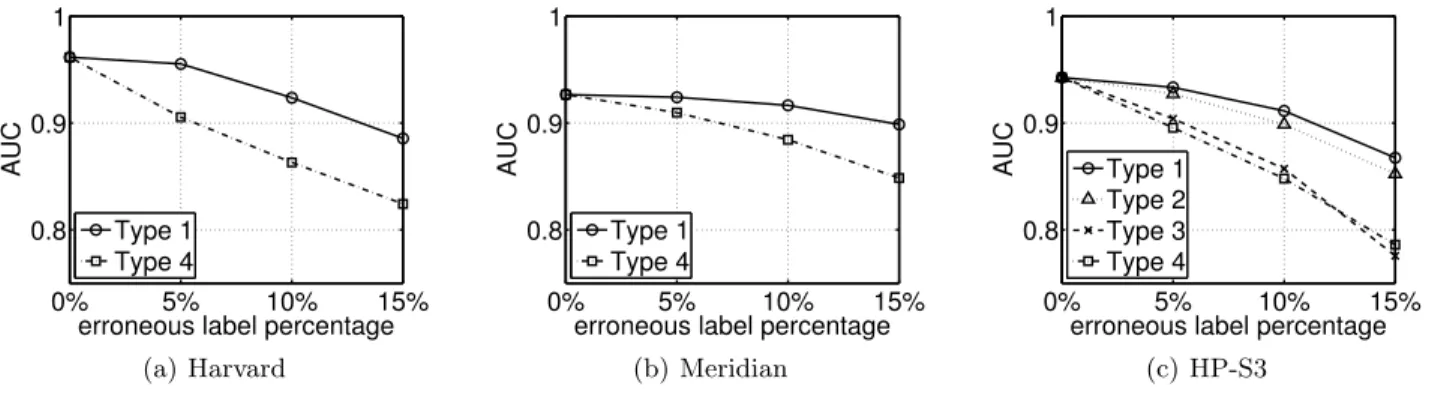
In particular, we simulated four different types of er-rors, including

Type 1: flip near τ. Flip randomly, with probability 0.5, the class labels of the paths with quantities within [τ − δ, τ + δ].

Type 2: underestimation bias. For ABW5_{, label}

er-roneously the paths with quantities within [τ, τ +δ] as “bad”.

Type 3: flip randomly. For ABW6_{, choose randomly}

5

Most ABW measurement tools such as pathload and pathchirp have a tendency of underestimating ABW [15], whereas such tendency is not reported by RTT measure-ment tools such as ping.

6

For most network measurements, “bad” paths are unlikely to be erroneously estimated as “good”. However, ABW is probed by the sender but inferred by the target node. Thus, malicious target nodes can purposely respond with flipped class labels.

p% paths and flip their labels.

Type 4: Good-to-Bad. Choose randomly p% “good” paths and label them as “bad”.

We experimented with all four types of errors for the HP-S3 dataset and the errors of Type 1 and 4 for the Harvard and Meridian datasets, shown in Figure 6. Dif-ferent error levels of 5%, 10% and 15% erroneous labels were tested by setting different δ’s and p’s for each type of errors and for each dataset. The values of δ are shown in Table 3 and p = 5, 10 and 15.

It can be seen that random errors of “flip randomly” and “Good-to-Bad” have a much larger impact to the classification accuracy than errors of “flip near τ” and “underestimation bias” that only perturb paths with quantities near τ. The random errors are mostly due to network anomalies. They are therefore rarer and can be addressed by incorporating heuristics such as inferring the class labels using some consensus based on recorded

(10)

0% 5% 10% 15% 0.8

0.9 1

erroneous label percentage

AUC Type 1 Type 4 (a) Harvard 0% 5% 10% 15% 0.8 0.9 1

AUC Type 1 Type 4 (b) Meridian 0% 5% 10% 15% 0.8 0.9 1

AUC Type 1 Type 2 Type 3 Type 4

(c) HP-S3

Figure 6: Robustness of class-based prediction against erroneous class labels. Table 2: Confusion Matrix

Harvard Accuracy=89.4%

Predicted “Good” “Bad” Actual “Good”_“Bad” 93.6%_14.7% _85.3%6.4%

Meridian Accuracy=85.4%

Predicted “Good” “Bad” Actual “Good”_“Bad” 88.5%_17.8% 11.5%_82.2%

HP-S3 Accuracy=87.3%

Predicted “Good” “Bad” Actual “Good”_“Bad” 93.5%_18.9% _81.1%6.5% Table 3: The values of δ that lead to certain error levels in Figure 6.

error%

δ

Harvard (ms) Meridian (ms) HP-S3 (Mbps)

Type 1 Type 1 Type 1 Type 2

5% 24.4 5.2 3.2 2.9

10% 41.5 10.2 6.7 5.7

15% 54.7 14.8 13.2 10.0

historical measurements. The errors of “flip near τ” and “underestimation bias” are mostly due to the inac-curacies of the measurement tools and can generally be reduced at the cost of more probe traffics, which is less necessary due to their limited impact.

6.4 Peer Selection:

Optimality VS. Satisfaction

For many Internet applications such as peer-to-peer downloading and streaming, the exploitation of end-to-end network performance is to find for each node a sat-isfactory node to interact with from a number of can-didates. Motivated by this demand, we demonstrate how peer selection can benefit from the prediction of network performance classes. We also compare

class-based and quantity-class-based prediction on peer selection using the same DMFSGD algorithms with the quantity-based prediction adopting the L2loss function and the

corresponding gradient functions in eqs. 18 and 19. To this end, we let each node randomly select a set of peers from all connected nodes. The nodes in the peer set are forced to be different from those in the neighbor set. For class-based prediction, we need to select the peer in the peer set which is the most likely to be “good”. This is done by selecting the peer with the largest predicted value, i.e., for node i,

jp= arg max

j∈PeerSet(i)ˆxij.

Note that we directly use the output of ˆxij = uivjT

with-out taking its sign or thresholding it by τc. For

quantity-based prediction, peer selection is done by choosing for each node the predicted best-performing node in the peer set, i.e., the smallest ˆxij for RTT and the largest

ˆxij for ABW. To demonstrate the impact of erroneous

labels to peer selection, we simulated 10% “flip near τ” and 5% “Good-to-Bad” errors, leading to overall 15% erroneous labels for all datasets. The random peer se-lection is used as a baseline method for comparison.

The commonly-used evaluation criterion for peer se-lection is the stretch [27], defined as

si= x_xi• i◦,

where • is the id of the selected peer, ◦ is that of the true best-performing peer in the peer set of node i and xi∗is

the measured quantity of some performance metric. si

is larger than 1 for RTT and smaller than 1 for ABW. The closer si is to 1, the better.

The stretch reflects the optimality of peer selection, shown in the first row of Figure 7. As expected, peer selection based on both class-based and quantity-based prediction outperforms random peer selection and the best optimality is achieved by using quantity-based pre-diction. Indeed, class-based prediction seeks to pro-vide satisfactory instead of optimal services. To demon-strate this, we plot the average percentage of unsatisfied

(11)

Harvard Meridian HP-S3 Optimalit y 10 20 30 40 50 60 0 5 10 15 20 25 30 35 40 peer number stretch Random Classification Regression Classification with noise

10 20 30 40 50 60 2 4 6 8 10 12 14 peer number stretch Random Classification Regression Classification with noise

10 20 30 40 50 60 0.55 0.6 0.65 0.7 0.75 0.8 0.85 peer number stretch Random Classification Regression Classification with noise

Satisfaction 10 20 30 40 50 60 0 0.1 0.2 0.3 0.4 0.5 peer number

unsatisfied node percentage

Random Classification Regression Classification with noise

10 20 30 40 50 60 0 0.1 0.2 0.3 0.4 0.5 peer number

10 20 30 40 50 60 0.05 0.1 0.15 0.2 0.25 0.3 peer number

Figure 7: Peer selection with various numbers of peers in the peer set of each node. The top row shows the optimality of the peer selection in terms of the average stretch, and the bottom row shows the satisfaction in terms of the average percentage of unsatisfied nodes, defined as the nodes that select wrongly “bad” peers when there exist “good” peers in the peer sets. The nodes with a peer set of all “bad” peers are excluded from the calculation as no satisfactory peers can be selected. nodes, defined as the nodes that select wrongly “bad”

peers when there are “good” peers available in the peer sets, shown in the second row of Figure 7. It can be seen that in terms of satisfaction, class-based predic-tion is sufficient to provide satisfactory services with about on average 10% unsatisfied nodes and as large as 15% erroneous labels only degrade the performance of peer selection by less than 5% for all datasets.

Note that quantity-based prediction achieved on HP-S3 a marginally better performance, less than 5%, on the percentage of unsatisfied nodes than class-based prediction, however at the cost of much more mea-surement overheads in order to get precise ABW val-ues. It should also be noted that always selecting best-connected nodes doesn’t make efficient use of the over-all capacity of the networks and may cause congestions and overloading to those nodes due to their popularity especially in the beginning of the services [6].

7. CONCLUSIONS AND FUTURE WORKS

This paper presents a novel approach to predicting end-to-end network performance classes. The success of the approach roots both in the qualitative represen-tation of network performance and in the exploration of the low-rank nature of performance matrices. The for-mer lowers greatly the measurement cost and enables a

unified treatment of various performance metrics, while the latter enjoys the recent advances in matrix com-pletion techniques, particularly the stochastic optimiza-tion which makes a fully decentralized processing pos-sible. Our so-called Decentralized Matrix Factorization by Stochastic Gradient Descent (DMFSGD) algorithms are highly scalable, able to deal with dynamic measure-ments in large-scale networks, while robust to erroneous measurements, which is the first of its kind.

While we focus here on binary classification, our frame-work could be extended to the prediction of more than two performance classes, i.e., multiclass classification, which we would like to study in the near future. The evaluation on peer selection shows the usability of our approach in real applications such as peer-to-peer file sharing and content distribution systems. In the future, we would also like to deploy one such system to test whether these applications can benefit from the simplic-ity, the flexibilsimplic-ity, and the superiority of our approach.

Acknowledgments

We thank Venugopalan Ramasubramanian for provid-ing us the HP-S3 dataset. We thank Augustin Chain-treau for shepherding this paper and the anonymous reviewers for their helpful feedback. This work was partially supported by the EU under project FP7-Fire

(12)

ECODE, by the European Network of Excellence PAS-CAL2 and by the Belgian network DYSCO (Dynamical Systems, Control, and Optimization), funded by the In-teruniversity Attraction Poles Programme, initiated by the Belgian State, Science Policy Office. The scientific responsibility rests with its authors.

8. REFERENCES

[1] D. Bertsekas. Nonlinear programming. Athena Scientific, 1999.

[2] C. M. Bishop. Pattern Recognition and Machine Learning. Springer-Verlag, New York, NJ, USA, 2006.

[3] L. Bottou. Online algorithms and stochastic approximations. In D. Saad, editor, Online Learning and Neural Networks. Cambridge University Press, 1998.

[4] A. M. Buchanan and A. W. Fitzgibbon. Damped newton algorithms for matrix factorization with missing data. In Computer Vision and Pattern Recognition, 2005.

[5] E. J. Cand`es and Y. Plan. Matrix completion with noise. Proc. of the IEEE, 98(6), 2010. [6] M. Crovella and B. Krishnamurthy. Internet

Measurement: Infrastructure, Traffic and

Applications. John Wiley & Sons, Inc., New York, NY, USA, 2006.

[7] F. Dabek, R. Cox, F. Kaashoek, and R. Morris. Vivaldi: A decentralized network coordinate system. In Proc. of ACM SIGCOMM, Portland, OR, USA, Aug. 2004.

[8] B. Donnet, B. Gueye, and M. A. Kaafar. A survey on network coordinates systems, design, and security. IEEE Communication Surveys and Tutorial, 12(4):488–503, 2010.

[9] Google TV. http://www.google.com/tv/. [10] M. Jain and C. Dovrolis. End-to-end available

bandwidth: measurement methodology, dynamics, and relation with TCP throughput. IEEE/ACM Transactions on Networking, 11:537–549, Aug. 2003.

[11] J. Ledlie, P. Gardner, and M. I. Seltzer. Network coordinates in the wild. In Proc. of USENIX NSDI, Cambridge, Apr. 2007.

[12] Y. Liao, P. Geurts, and G. Leduc. Network distance prediction based on decentralized matrix factorization. In Proc. of IFIP Networking Conference, Chennai, India, May 2010. [13] Y. Mao, L. Saul, and J. M. Smith. IDES: An

Internet distance estimation service for large networks. IEEE Journal On Selected Areas in Communications, 24(12):2273–2284, Dec. 2006. [14] T. S. E. Ng and H. Zhang. Predicting Internet

network distance with coordinates-based approaches. In Proc. of IEEE INFOCOM, New

York, NY, USA, June 2002.

[15] R. S. Prasad, M. Murray, C. Dovrolis, K. Claffy, R. Prasad, and C. D. Georgia. Bandwidth

estimation: Metrics, measurement techniques, and tools. IEEE Network, 17:27–35, 2003.

[16] V. Ramasubramanian, D. Malkhi, F. Kuhn, M. Balakrishnan, A. Gupta, and A. Akella. On the treeness of Internet latency and bandwidth. In ACM SIGMETRICS / Performance, Seattle, WA, USA, June 2009.

[17] S. Ratnasamy, P. Francis, M. Handley, R. Karp, and S. Shenker. A scalable content-addressable network. In Proc. of ACM SIGCOMM, San Diego, CA, USA, Aug. 2001.

[18] S. Ratnasamy, M. Handley, R. Karp, and S. Shenker. Topologically-aware overlay construction and server selection. In Proc. of

IEEE INFOCOM, June 2002.

[19] V. J. Ribeiro, R. H. Riedi, R. G. Baraniuk, J. Navratil, and L. Cottrell. pathchirp: Efficient available bandwidth estimation for network paths. In Proc. of the Passive and Active Measurement, 2003.

[20] I. Rish and G. Tesauro. Estimating end-to-end performance by collaborative prediction with active sampling. In Integrated Network Management, pages 294–303, May 2007. [21] A. Shriram, M. Murray, Y. Hyun, N. Brownlee,

A. Broido, M. Fomenkov, and K. Claffy. Comparison of public end-to-end bandwidth estimation tools on high-speed links. In Proc. of the Passive and Active Measurement, pages 306–320, 2005.

[22] N. Srebro, J. D. M. Rennie, and T. S. Jaakola. Maximum-margin matrix factorization. In Advances in Neural Information Processing Systems, pages 1329–1336, 2005.

[23] L. Tang and M. Crovella. Virtual landmarks for the Internet. In Proc. of ACM/SIGCOMM Internet Measurement Conference, Oct. 2003. [24] Vuze Bittorrent. http://www.vuze.com/. [25] B. Wong, A. Slivkins, and E. Sirer. Meridian: A

lightweight network location service without virtual coordinates. In Proc. of ACM SIGCOMM, Aug. 2005.

[26] P. Yalagandula, P. Sharma, S. Banerjee, S. Basu, and S.-J. Lee. S3: a scalable sensing service for monitoring large networked systems. In Proc. of the 2006 SIGCOMM workshop on Internet network management, pages 71–76, 2006. [27] R. Zhang, C. Tang, Y. C. Hu, S. Fahmy, and

X. Lin. Impact of the inaccuracy of distance prediction algorithms on Internet applications: an analytical and comparative study. In Proc. of IEEE INFOCOM, Barcelona, Spain, Apr. 2006.