TWO-WAY FLUID-STRUCTURE COUPLING METHODOLOGY FOR MODELING 3D FLEXIBLE HYDROFOILS IN VISCOUS FLOW
ZAHRA MORTAZAVINIA
DÉPARTEMENT DE GÉNIE MÉCANIQUE ÉCOLE POLYTECHNIQUE DE MONTRÉAL
THÈSE PRÉSENTÉE EN VUE DE L’OBTENTION DU DIPLÔME DE PHILOSOPHIÆ DOCTOR
(GÉNIE MÉCANIQUE) AOÛT 2018
c
ÉCOLE POLYTECHNIQUE DE MONTRÉAL
Cette thèse intitulée :
TWO-WAY FLUID-STRUCTURE COUPLING METHODOLOGY FOR MODELING 3D FLEXIBLE HYDROFOILS IN VISCOUS FLOW
présentée par : MORTAZAVINIA Zahra
en vue de l’obtention du diplôme de : Philosophiæ Doctor a été dûment acceptée par le jury d’examen constitué de :
M. REGGIO Marcelo, Ph. D., président
M. CAMARERO Ricardo, Ph. D., membre et directeur de recherche M. GUIBAULT François, Ph. D., membre et codirecteur de recherche M. TRÉPANIER Jean-Yves, Ph. D., membre
DEDICATION
To my family for their sincere love. . .
ACKNOWLEDGEMENTS
First and foremost, I would like to express my sincere gratitude to my advisors Professor Ricardo Camarero and Professor François Guibault for the continuous support of my Ph.D study and research, for their patience, motivation, enthusiasm, and immense knowledge. Their guidance helped me in all the time of research and writing of this thesis.
My time in Montreal was made enjoyable in large part due to the many friends and groups that became a part of my life. I am grateful for time spent with all of them and our memorable moments. I warmly thank Mr. Mojtaba Mirzaei and Mr. Soheil Namvar, for their valuable advices and helps during my study.
Computations are made on the supercomputers "Briarée" from "Université de Montréal", and "Guillimin" from "McGill University", managed by Calcul Québec and Compute Canada. The operation of this supercomputer is funded by the Canada Foundation for Innovation (CFI), the ministère de l’Économie, de la science et de l’innovation du Québec (MESI) and the Fonds de recherche du Québec - Nature et technologies (FRQ-NT).
Last, but definitely not the least by any measure, I would like to acknowledge with deepest gratitude, support from my family. My parents have been a constant source of inspiration throughout my life. I would like to express my exceptional gratitude to my sister and brother, Sepideh and Amir, for their continuous and loving support. I am indebted to my husband, Sina, who supported my research with his patience and of course for his knowledge on the fluid mechanics. I would like to thank my son, Kian, who brought shine, joy and motivation to my life.
RÉSUMÉ
Les surfaces portantes. telles que des pâles, ailes, et hydrofoil sont sujets à des instabilités comme la divergence, le battement et la résonnance qui peuvent provoquer la fatigue de la structure et réduire sa tenue en service. Par conséquent, il est important de comprendre et de prédire avec précision la réponse et la stabilité de telles structures afin d’en assurer la sécurité, et de faciliter la conception et optimisation de concepts nouveaux et existants. L’interaction entre un écoulement et une structure, nommée interaction fluide-structure (IFS), doit être prise en compte lors de l’étude la réponse élastique et des instabilités de surfaces portantes. Pour de telles applications, l’écoulement et la structure sont couplés au travers de la charge qui s’exerce sur la structure par le fluide, et la déformation qui en découle. Pour certaines applications IFS, le fluide et le solide peuvent être couplés par un transfert uni-directionnel de la charge. Dans ce cas, un champ donné peut fortement affecter l’autre sans l’être lui même. Cependant, pour certaines applications en ingénierie, où il y a une relation forte et potentielement nonlinéaire entre ces champs, un couplage uni-directionnel n’est pas adéquat. Alors, les déplacements de la structure causés par l’écoulement accentuent les forces du fluide de telle sorte que le fuide et la structure intéragissent en boucle de facon complexe. Donc, une analyse bi-directionnelle doit être entreprise.
Les structure légères et flexibles sont courament utilisées grâce aux avancées récentes dans les technologies des matériaux afin d’améliorer les caractéristiques hydrodynamiques et struc-turelles par rapport aux matériaux lourds et rigides. Dans cette thèse, on cherche une meilleure compréhension de la phénomènologie hydroélastique d’hydrofoils hautement flex-ibles, qui subissent de grandes déformations sous de fortes charges. Ceci milite en faveur d’une méthodologie IFS bi-directionnelle fortement couplée, en plus de l’incorporation de techniques numériques avancées pour la modélisation de la déformation de maillages adap-tés.
Pour des nombres de Reynolds moyens à élevés, le dévelopement d’un écoulement turbu-lent autour de l’hydrofoil provoque un transfert du mouvement perpendiculaire à la paroi et permet à l’écoulement de se re-attacher, et ainsi former une bulle laminaire de séparation ( Laminar Separation Bubble, LSB). Le décrochage de l’écoulement, la formation de tour-billons dans le sillage, la localisation et le mouvement de la bulle laminaire sont tous des phénomènes qui affectent les charges hydrodynamiques et les vibrations de la structure. Par conséquent, une méthodologie numérique avancée, avec une précision spatiale suffisamenent élevée a été incorporée dans ce travail pour capturer finement ces phénomènes à l’interface
fluide-structure, tels que l’apparition et l’étendue de la zone de séparation.
L’interaction entre la surface portante et l’écoulement environnant implique d’importantes caractéristiques tri-dimensionnelles qui ne seront pas négligées dans cette thèse. Par ex-emple, les effets visqueux, la séparation, le sillage et le décrochage de tourbillons dont les effets directs ont été démontrés pour établir les charges hydrodymaniques, sont à l’origine de tels effets tri-dimensionnels qui doivent être pris en compte pour améliorer la précision de la modélisation d’écoulements turbulents. À cause de la déformation due au flèchisse-ment et à la torsion de la surface, la charge hydrodynamique n’est pas uniforme dans la direction de l’envergure. En particulier, pour une surface portante flexible soumise à des écoulements à grandes vitesses et incidences élevées, la déformation élastique est importante, et par conséquent, ces caractéristiques tri-dimensionnelles ne peuvent plus être négligées. Dans cette thèse, on propose une méthodologie avancée d’interaction fluide-structure bi-directionnelle fortement couplée pour étudier la réponse hydro-élastique de surfaces portantes légères et flexibles, et tri-dimensionnelles, dans des écoulements visqueux à des nombres de Reynolds moyens à élevés. Le problème de l’interaction fluide-structure est résolu par un logiciel de résolution numérique par volumes finis pour la partie fluide, CFX, et un code d’éléments finis, ANSYS, pour la partie solide du domaine. Au cours des simulations forte-ment couplées, les résoluteurs fluide et solide exécutent une suite d’étapes multi-champs, chacune comprenant un ou plusieurs couplages itératifs.
Le résoluteur fluide visqueux et le résoluteur IFS couplé sont tous deux validés par des com-paraisons avec des résultats numériques et des mesures expérimentales. Pour quantifier les effets IFS, l’étude porte sur des hydrofoils rigides (en acier inoxydable) et flexibles (Polyac-etate POM) avec la même géométrie non-déformée. La déformation due à l’écoulement ainsi que la réponse élastique de ces structures sous plusieurs conditions (vitesses amont, angles d’incidence) pour des nombres de Reynolds moyens à élevés, sont étudiées.
ABSTRACT
Lifting bodies, such as blades, wings, and hydrofoils, may be subject to instabilities, such as divergence, flutter, and resonance, which can fatigue the structure and reduce its operational longevity. Therefore, it is important to understand and accurately predict the response and stability of such structures to ensure their structural safety and facilitate the design and optimization of new and existing concepts.
The interaction between fluid and structure, known as Fluid-Structure Interaction (FSI), should be taken into account in the study of elastic response and instabilities of flexible lifting bodies. In such applications, the fluid flow and structure are coupled through the loads exerted on the structure by the fluid, which results in the the structural deformation. In some FSI applications, fluid and solid can be coupled by one-way (unidirectional) load transfer. In this case, a given field may strongly affect, but not be affected significantly by the other field. However, for some practical engineering applications, in which there is a strong and potentially nonlinear relationship between the fields, one-way coupling is not adequate. In such cases, the structural displacement caused by the flow further enhances the fluid forces in such a way that both fluid and structure are interacting in a complex feedback fashion. Hence, two-way FSI analysis needs to be undertaken.
Light-weight, flexible structures are widely used through recent advances in material tech-nologies to improve hydrodynamic and structural performance compared to heavy and stiff materials. This project seeks to gain greater insight into the hydroelastic response of highly flexible hydrofoils, which undergo large deformation when subjected to high hydrodynamic loadings. This increases the necessity of incorporating strongly-coupled two-way FSI method-ology in addition to the numerical challenges in mesh deformation modelling.
At moderate to high Reynolds numbers, the development of turbulent flow around a hydrofoil causes a momentum transfer normal to the wall and allows the flow to re-attach, and form a Laminar Separation Bubble (LSB). Flow separation, formation of trailing edge vortices, location and movement of the LSB affect the hydrodynamic loading and structural vibration. Hence, an advanced numerical technique with sufficiently high spatial accuracy is incorpo-rated in the present study to precisely capture these local interface phenomena, such as the onset and the amount of flow separation.
The interaction between the foil and surrounding flow involve significant three-dimensional features that will not be neglected in the present study. For instance, the viscous effects, separation, wakes and vortex shedding, which have been shown to have immediate effects
in determination of hydrodynamic loads on hydofoils, have significant 3D features that have to be accounted for to improve the accuracy of turbulent modelling. Due to the bending and twist deformation of the foil, the hydrodynamic loading is not uniform along the span-wise direction. Particularly, for a flexible foil subjected to high flow velocities at hich angles of attacks, the elastic deformation is significant and hence, these 3D features cannot be neglected.
This PhD project proposes an advanced strongly-coupled two-way fluid-structure interaction methodology to investigate hydroelastic response of three-dimensional lightweight flexible hydrofoils in viscous flow at moderate to high Reynolds number. The fluid-structure problem is solved with a finite volume-based code for the fluid domain, CFX, and a finite element-based code, ANSYS, for the structural domain. During the strongly-coupled simulations, the fluid and structural solvers execute the simulation through a sequence of multifield steps, each of which consists of one or more coupling iterations.
The viscous fluid solver and the coupled FSI solver are both validated by comparing the numerical results with measured experimental data. To quantify the FSI effects, rigid (stain-less steel) and flexible (POM Polyacetate) hydrofoils with the same undeformed geometry are simulated and compared. The flow-induced deformation and elastic response of those structures at various operating conditions, i.e. inlet velocities and angles of attack, subjected to moderate to high Reynolds number flows will be studied.
TABLE OF CONTENTS DEDICATION . . . iii ACKNOWLEDGEMENTS . . . iv RÉSUMÉ . . . v ABSTRACT . . . vii TABLE OF CONTENTS . . . ix LIST OF TABLES . . . xi
LIST OF FIGURES . . . xii
LIST OF APPENDICES . . . xvi
CHAPTER 1 INTRODUCTION . . . 1
1.1 Motivation . . . 1
1.2 Research goal . . . 4
1.3 Thesis overview and organization . . . 4
CHAPTER 2 LITERATURE REVIEW . . . 6
2.1 Physical instability modes . . . 6
2.2 Viscous effects . . . 8
2.3 Fluid-structure interaction . . . 10
2.4 Reasons for 3D simulation . . . 17
2.5 Objectives . . . 19
CHAPTER 3 THEORETICAL BACKGROUND . . . 20
3.1 Numerical modeling of Fluid-structure interaction . . . 20
3.1.1 Monolithic approach . . . 20
3.1.2 Partitioned approach . . . 21
3.1.3 FSI modeling in ANSYS . . . 22
3.2 Governing equations . . . 25
3.2.1 Fluid domain . . . 25
CHAPTER 4 DESCRIPTION OF THE TEST CASE . . . 40 4.1 Geometry selection . . . 40 4.2 Fluid domain . . . 41 4.3 Structural domain . . . 42 4.4 Boundary conditions . . . 43 CHAPTER 5 METHODOLOGY . . . 45
5.1 Numerical set-up: fluid domain . . . 45
5.1.1 Inlet velocity . . . 47
5.1.2 Undeformed (initial) mesh . . . 48
5.1.3 Mesh deformation . . . 48
5.1.4 Time step setting . . . 58
5.1.5 Solver controls . . . 59
5.2 Validation of the viscous fluid solver . . . 59
5.3 Numerical set-up: structural domain . . . 62
5.4 Mesh convergence study . . . 63
5.5 Validation of the two-way FSI solver . . . 66
5.6 Comparison of one-way and two-way coupling methods for FSI analysis of the flexible hydrofoils . . . 68
5.7 Transition modelling: effects on laminar to turbulent transition . . . 71
CHAPTER 6 RESULTS . . . 77
6.1 Flow-induced deformation of the flexible hydrofoil . . . 77
6.2 Pressure coefficient distribution at the hydrofoil tip . . . 78
6.3 Flow patterns . . . 79
6.4 Lift and drag coefficients . . . 81
6.5 Pressure coefficient distribution along the span-wise direction . . . 83
CHAPTER 7 CONCLUSION . . . 93
7.1 Summary . . . 93
7.2 Limitations and future work . . . 94
REFERENCES . . . 96
LIST OF TABLES
Table 4.1 Material properties of the rigid and flexible hydrofoils . . . 42 Table 5.1 Acceptable ranges of mesh quality measures in CFX . . . 50 Table 5.2 Lift coefficient convergence as a function of number of nodes on the
hydrofoil profile in the stream-wise direction (Nf oil) . . . 65
Table 5.3 Lift coefficient convergence as a function of number of elements in the span-wise direction (nspan) . . . 66
Table 5.4 Comparison of the experimental (Akcabay et al., 2014) and computa-tional lift and drag coefficients and the tip section displacement for the rigid and flexible hydrofoils at α=8◦ . . . 68 Table 5.5 Comparison of the lift and drag coefficients for NACA0012 airfoil at
α=18◦ and Re = 4 × 10⁶, with and without transition modeling . . . 75 Table 6.1 Comparison of the minimum pressure coefficient for the rigid and
LIST OF FIGURES
Figure 1.1 Schematic of the field of hydroelasticity (from (Hodges and Pierce,
2004) adapted to hydroelasticity) . . . 2
Figure 2.1 Flow separating from a foil and stall at high angles of attack (Wikipedia, 2018) . . . 7
Figure 2.2 The wake pattern of a NACA0009 hydrofoil for four values of the re-duced frequency, κ, (Munch et al., 2010) . . . . 9
Figure 2.3 Dynamics of a 2D hydrofoil cross section with two DOF (Ducoin and Young, 2013) . . . 14
Figure 2.4 A two-degrees-of-freedom model representing plunging and pitching (ω(t) and θ(t)) of a 2D hydrofoil (Lefrançois, 2017) . . . . 15
Figure 2.5 NACA0015 POM hydrofoil inside the tunnel (Chae et al., 2016) . . . 18
Figure 3.1 Monolithic approach (Raja, 2012) . . . 20
Figure 3.2 Partitioned approach (Raja, 2012) . . . 21
Figure 3.3 One-way coupling . . . 22
Figure 3.4 Two-way coupling . . . 23
Figure 3.5 Sequence of synchronization points in ANSYS multifield solver (Refer-ence: ANSYS User Guide) . . . 24
Figure 3.6 Subdivisions of the near-wall region (Reference: ANSYS User Guide) 32 Figure 4.1 The experimental set-up for NACA66 flexible hydrofoil in Ref. (Ak-cabay et al., 2014) . . . 41
Figure 4.2 3D domain of the computational fluid dynamics solver . . . 42
Figure 4.3 Solid domain . . . 43
Figure 5.1 (a) Domain 1 corresponds to experimental facility for use in the vali-dation of the results; (b) The infinite-like boundary domain (Domain 2) . . . 46
Figure 5.2 Inlet velocity . . . 47
Figure 5.3 Fluid mesh details . . . 49
Figure 5.4 Undeformed mesh and the expansion factor, u0= 15m/s . . . 51
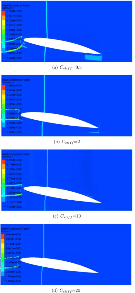
Figure 5.5 Effects of the stiffness model exponent, Cstif f, on the expansion factor of the deformed mesh for flows with u0= 15m/s . . . . 52
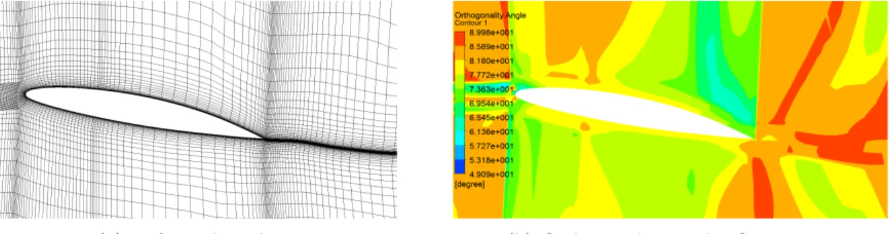
Figure 5.6 Undeformed mesh and the orthogonality angle, u0= 5m/s . . . 53
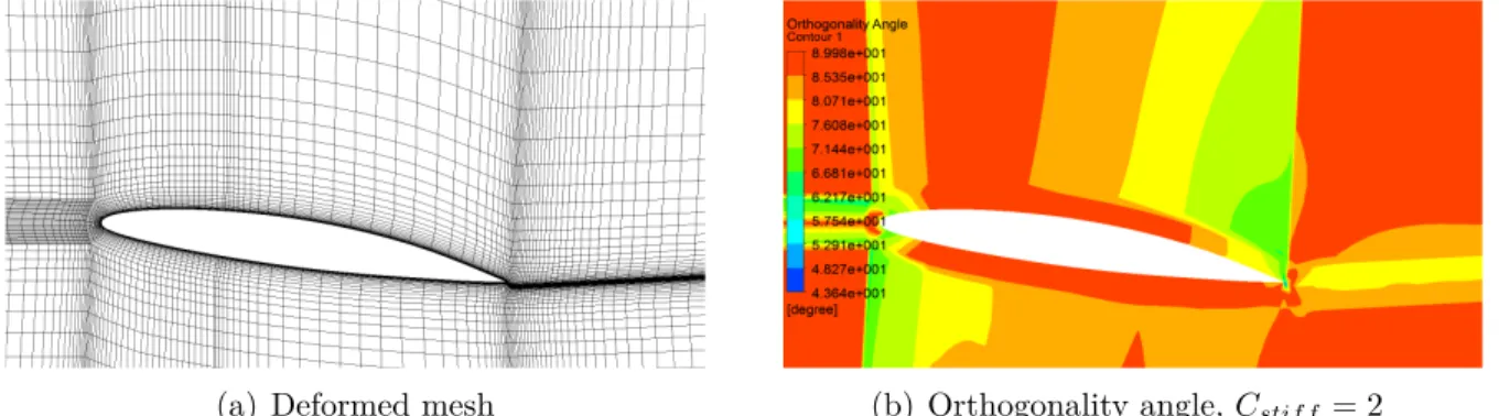
Figure 5.7 Deformed mesh and the orthogonality angle, increasing the stiffness near small volumes with Cstif f = 2, u0= 5m/s . . . . 53
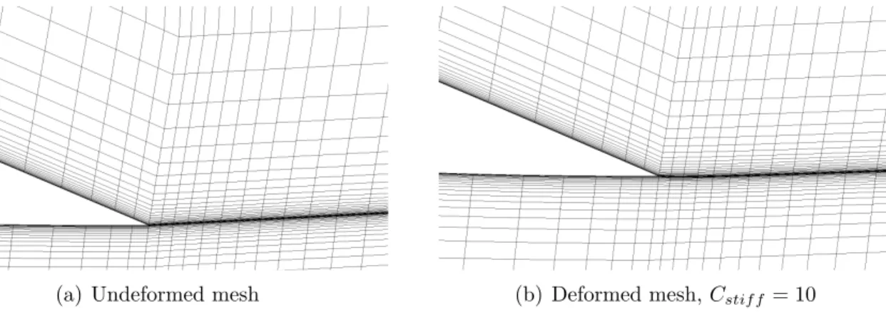
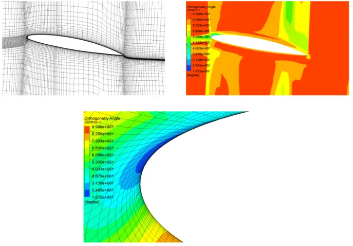
Figure 5.8 Comparison of the undeformed and deformed mesh near the trailing edge, Cstif f = 2, u0= 5m/s . . . . 54 Figure 5.9 Deformed mesh and the orthogonality angle, increasing the stiffness
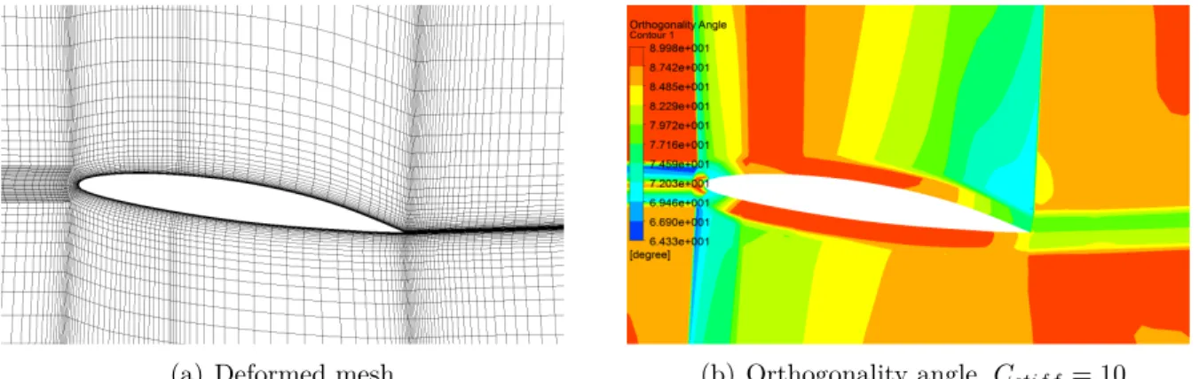
near small volumes with Cstif f = 10, u0= 5m/s . . . . 54 Figure 5.10 Comparison of the undeformed and deformed mesh near the trailing
edge, Cstif f = 10, u0= 5m/s . . . . 55 Figure 5.11 Deformed mesh and the orthogonality angle, increasing the stiffness
near small volumes with Cstif f = 2, u0= 15m/s . . . . 55 Figure 5.12 Deformed mesh and the orthogonality angle, increasing the stiffness
near small volumes with Cstif f = 1, u0= 15m/s . . . . 56 Figure 5.13 Deformed mesh and the orthogonality angle, increasing the stiffness
near small volumes with Cstif f = 10, u0= 15m/s . . . 56 Figure 5.14 Deformed mesh and the orthogonality angle, increasing the stiffness
near small volumes with Cstif f = 20, u0= 15m/s . . . 57 Figure 5.15 Deformed mesh and the orthogonality angle, increasing the stiffness
near small volumes with Cstif f = 10, u0= 20m/s . . . 58 Figure 5.16 Comparison of experimental (Gregory and O’Reilly, 1970) and
numer-ical pressure coefficient, Cp, on a NACA0012 foil for Reynolds number
of Re = 2.88 × 10⁶ . . . 60 Figure 5.17 Comparison of experimental (Ladson, 1988) and numerical lift
coeffi-cients, CL, on a NACA0012 foil for different Reynolds numbers as a
function of the angle of attack, α . . . . 61 Figure 5.18 Comparison of experimental (Ladson, 1988) and numerical drag
coef-ficients, CD, on a NACA0012 foil for different Reynolds numbers as a
function of the angle of attack, α . . . . 62 Figure 5.19 The structural mesh used for CSD simulation . . . 63 Figure 5.20 Pressure coefficient, Cp, along the hydrofoil surface for the rigid foil at
α=8◦ for different values of Y+. (Nf oil=400 and nspan=40 ) . . . 64
Figure 5.21 Pressure coefficient, Cp, along the foil surface for the rigid hydrofoil at
α= 8◦ for different values of Nf oil. (Y+=1 and nspan=40 ) . . . 65
Figure 5.22 Comparison of the experimental (Akcabay et al., 2014) and computa-tional pressure coefficient, Cp, along the free tip of the rigid hydrofoil
surface at α=8◦ . . . 67 Figure 5.23 Comparison of the total displacement for the flexible hydrofoil at α =
8◦ with one-way (left column) and two-way (right column) coupling methods . . . 70
Figure 5.24 Comparison of the vertical tip section displacement, δy, for the flexible
hydrofoil at α = 8◦ with one-way and two-way coupling methods . . . 71 Figure 5.25 Comparison of the velocity contours for the flexible hydrofoil at α =
8◦ with one-way (left column) and two-way (right column) coupling methods . . . 72 Figure 5.26 Comparison of (a) lift coefficient (b) drag coefficient of flexible
hydro-foils at α = 8◦ with one-way and two-way coupling methods . . . 73 Figure 5.27 Skin friction coefficient along the hydrofoil upper surface for the flexible
hydrofoil at α=6◦ with u0= 20m/s . . . . 74 Figure 5.28 Skin friction coefficient along the hydrofoil upper surface for the flexible
hydrofoil at α=6◦ with u0= 25m/s . . . . 75 Figure 5.29 Comparison of the velocity contours at the free tip of the flexible
hy-drofoil at α=6◦ with u0= 25m/s with and without transition modeling 76 Figure 5.30 Comparison of the streamlines for a NACA0012 airfoil at α=18◦ and
Re = 4 × 10⁶, with and without transition modeling . . . . 76 Figure 6.1 Total mesh displacement contour for the flexible hydrofoil at α=8◦ with
u0= 5m/s . . . . 78 Figure 6.2 Total mesh displacement contour for the flexible hydrofoil at α=8◦ with
u0= 20m/s . . . 78 Figure 6.3 The vertical tip section displacement, δy, for the flexible hydrofoil at
various angles of attack . . . 79 Figure 6.4 Pressure coefficient, Cp, for the rigid and flexible hydrofoils subjected
to flow with u0= 10m/s at: (a) α=2◦, (b) α=4◦, (c) α=6◦ and (d)α=8◦ 80 Figure 6.5 Pressure coefficient, Cp, for the rigid and flexible hydrofoils subjected
to flow with u0= 15m/s at: (a) α=2◦, (b) α=4◦, (c) α=6◦ and (d)α=8◦ 81 Figure 6.6 Pressure coefficient, Cp, for the rigid and flexible hydrofoils subjected
to flow with u0= 20m/s at: (a) α=2◦, (b) α=4◦ and (c) α=6◦ . . . . 83 Figure 6.7 Pressure coefficient, Cp, for the rigid and flexible hydrofoils subjected
to flow with u0= 25m/s at: (a) α=2◦, (b) α=4◦ and (c) α=6◦ . . . . 84 Figure 6.8 Laminar to turbulent transition and the laminar separation bubble for
u0= 5m/s . . . . 85 Figure 6.9 Comparison of the velocity contours at the free tip of the rigid (left
col-umn) and flexible (right colcol-umn) hydrofoils at various angles of attack,
Figure 6.10 Comparison of the velocity contours at the free tip of the rigid (left col-umn) and flexible (right colcol-umn) hydrofoils at various angles of attack,
α, for flow with u0= 20m/s . . . . 87 Figure 6.11 Comparison of the velocity contours at the free tip of the rigid (left
col-umn) and flexible (right colcol-umn) hydrofoils at various angles of attack,
α, for flow with u0= 25m/s . . . . 88 Figure 6.12 Lift coefficient for rigid and flexible hydrofoils as a function of the angle
of attack . . . 89 Figure 6.13 Drag coefficient for rigid and flexible hydrofoils as a function of the
angle of attack . . . 89 Figure 6.14 Lift coefficient for rigid and flexible hydrofoils as a function of the angle
of attack for different values of inlet velocities . . . 90 Figure 6.15 Drag coefficient for rigid and flexible hydrofoils as a function of the
angle of attack for different values of inlet velocities . . . 90 Figure 6.16 Pressure distribution along the hydrofoil surface at four sections in the
span-wise direction for the flexible hydrofoil at α=6◦ . . . 91 Figure 6.17 Pressure distribution along the hydrofoil surface at four sections in the
LIST OF APPENDICES
CHAPTER 1 INTRODUCTION
1.1 Motivation
Aeroelastic/hydroelastic behaviour of flexible lifting bodies, such as propulsors, blades and wings, is a very active area of research in the fields of aero/hydrodynamics, structural dynam-ics, and acoustics. From the fluid dynamics point of view, the dynamic loading on a blade, for instance, is affected by the motion of the blade, as given in classic texts such as aeroelastic theory by Theodorsen (Theodorsen, 1935). This unsteady loading causes time-dependent lift and drag forces that can lead to instabilities if not carefully controlled (Chae et al., 2013; Liaghat et al., 2014; Ducoin and Young, 2013). Structurally, these uncontrolled static or dynamic instabilities can lead to vibration, noise issues, excessive deformation, accelerated fatigue, and even catastrophic structural failures (Coutu et al., 2004, 2005, 2007; Seeley et al., 2012; Thapa et al., 2012; Liaghat et al., 2014). Structural vibration causes acoustic wave propagation in the fluid domain that can travel into the far-field and cause structural dam-age given enough energy (Reese, 2010). An important step towards the prediction of such structural damage consists in studying and precisely predicting material response to ensure the structural safety and to facilitate the design/optimization of new/existing structures. In the majority of earlier studies on the interaction between flexible lifting bodies and the surrounding flows, the focus has been on aerospace or wind energy applications, in which fluid damping and inertia have a limited effect on the solid. However, in the interaction between fluid and hydraulic turbines or marine propeller blades for instance, the influence of fluid inertia and fluid damping can be much more important. In those cases, the fluid viscous effects can significantly affect and interact with the dynamic response of the structures and must be taken into account in the analysis and design of such equipments.
Hydroelasticity
Hydroelasticity is the term used to denote the field of study concerned with the interaction between the change in shape of a deformable structure subjected to a fluid flow and the resulting hydrodynamic forces.
The interdisciplinary nature of the field is illustrated in Fig. 1.1 which represents the rela-tionships between the three disciplines of hydrodynamics, dynamics and elasticity, i.e. each circle represents a field of study related to hydroelasticity. The classical hydrodynamic theo-ries, adapted from aerodynamics (Hodges and Pierce, 2004; Harwood et al., 2016), provide a
prediction of the forces acting on a structure of a given shape. Elasticity provides a prediction of the shape of a deformable structure under a given load. Dynamics describes the effects of inertial forces. hydroelasticity dynamic hydroelasticity static flight mechanics structural dynamics
hydrodynamics
dynamics
elasticity
Figure 1.1 Schematic of the field of hydroelasticity (from (Hodges and Pierce, 2004) adapted to hydroelasticity)
The areas where these circles overlap represent the interaction between the relevent domains of study (Hutchison, 2012). Overlap between:
• elasticity and dynamics subfields represents structural dynamics; • fluid dynamics and dynamics represents flight mechanics;
• fluid dynamics and elasticity represents static hydroelasticity, in which the inertial forces have little effect; and,
• all the three subfields represents dynamic hydroelasticity, in which the inertial forces become more significant and phenomena such as flutter can occur.
It is not always easy to distinguish between static and dynamic hydroelasticity as the change can be dictated by the point at which the inertial interaction becomes significant, and may cause instability in the system dynamics (Hutchison, 2012). Hydroelasticity can be considered as the analysis of time-dependent interaction of hydrodynamic and elastic structural forces.
Fluid-Structure Interaction
Fluid–Structure Interaction (FSI) is a broad term spanning many engineering applications, but generally denotes the bidirectional energy transfer in a domain consisting of both fluid and structure (Liaghat et al., 2014). From both theoretical and practical points of view, the complex interaction between flow and structure, known as fluid–structure interaction, must be taken into account in the study of the elastic response and instabilities of flexible lifting bodies. In such applications, the fluid flow and structure are coupled through the force exerted on the structure by the fluid, which results in the structure deformation leading to a change of its orientation to the flow. The orientation and velocity of the structure relative to the fluid flow determines the fluid forces that will be exerted on the structure in a feedback system.
At the boundary between fluid and structure, known as the fluid-structure interface, infor-mation for the solution is shared between the fluid and structural solvers. The inforinfor-mation exchanged is dependent on the coupling method. In a one-way coupling, it is assumed that one domain is driven by the other, with the driven domain having no feedback effect on the driving domain. This method, however, is not always adequate for practical engineering ap-plications, in which the structural displacement caused by the flow further enhances the fluid forces in such a way that both fluid and structure are interacting in a complex feedback fash-ion. In such cases, two-way FSI analysis needs to be undertaken. Numerically, weak coupling methods are explicit and hence, suffer from possible instabilities. Strong coupling methods, in which equilibrium is satisfied jointly between fluid and structure in each time step, provide better fidelity. To the best of our knowledge, most of the numerical studies on flow over hy-drofoils thus far have focused primarily on problems with weak FSI. In the present study, a strongly coupled two-way FSI methodology will be presented to tackle the large flow-induced deformation and accurately simulate the subsequent complex flow phenomena.
Through recent advances in material technologies, it is possible to take advantage of lightweight, flexible hydrofoils to improve hydrodynamic and structural performance. Physical material properties of the structure (density, Young’s modulus and Poisson’s ratio) are important fac-tors in determination of the elastic deformation and, hence, have immediate effect on how strongly the fluid and structure are coupled in the FSI simulation. Physically, under a spec-ified hydrodynamic loading, a more flexible structure undergoes larger deformation. Such a large deformation requires a two-way coupling method, which leads to additional challenges in mesh deformation modelling. To the best of our knowledge, most of the former studies on the dynamic response of hydrofoils thus far involved hydrofoils made of relatively heavy and stiff materials, such as lead, stainless steel and aluminium. In the present study, a highly
flexible hydrofoil will be studied.
The interaction between the hydrofoil and the surrounding flow involves significant three-dimensional features, such as separation, wakes and vortex shedding, that have been shown to have immediate effects in the determination of hydrodynamic loads on hydofoils. Due to the bending and twist deformation of the foil, the hydrodynamic loading is not uniform along the span-wise direction. Particularly, for a flexible foil subjected to high flow velocities at high angles of attacks, the elastic deformation is significant and hence, these 3D features cannot be neglected. Most of the previous studies on the hydroelastic response of hydrofoils have focused mainly on 2D simulations, where the 3D features are neglected. In the present study, we will emphasize these 3D features.
1.2 Research goal
Even though several numerical techniques have been developed to simulate fluid-structure interaction of hydrofoils and provide precise prediction of their hydroelastic response, there still remain some issues that require further investigation. Special care must be taken for the multiphysics nature of the problem which requires implementation of proper numerical techniques for capturing both the global hydroelastic response, and also very local phenomena at the interface, such as development and movement of Laminar Separation Bubble (LSB) that has been shown to have immediate effects on the hydroelastic response of the structure. The goal of this research is to develop an advanced strongly-coupled two-way fluid-structure interaction methodology with sufficiently high spatial accuracy to investigate hydroelastic response of a three-dimensional lightweight flexible hydrofoil in viscous flows. The flow-induced deformation and elastic response of those structures at various operating conditions, i.e. inlet velocities and angles of attack, subjected to moderate to high Reynolds number flows will be studied.
1.3 Thesis overview and organization
Following the present introduction, Chapter 2 provides a literature review on FSI response and stability of hydrofoils. This chapter will provide the context for additional research in the field of hydroelasticty at high Reynolds number flows and presents the different numerical methods to study fluid-structure interaction along with their advantages and drawbacks according to the literature. Furthermore, this chapter will illustrate the lack of an adequate account of three-dimensional features in this field. In Chapter 3, the fundamental concepts of fluid and solid mechanics as a necessary background for the fluid-structure analysis are
reviewed. This chapter includes a brief theoretical description of numerical modelling of FSI and the governing equations for the fluid and the structural domain. The test cases used for validation of the proposed methodology will be described in Chapter 4. The numerical modeling, including the fluid and solid models, meshes and boundary conditions are described in this chapter. In chapter 5, the proposed methodology will be presented. Chapter 6 provides a general discussion about the results. Finally, Chapter 7 presents the conclusion and contributions of the thesis followed by recommendations for future studies.
CHAPTER 2 LITERATURE REVIEW
In this chapter, we aim to provide a literature review to situate our research topic in relation to previous studies and present the current state of the art, upon which our study will build. First, the instability modes of a structure subjected to different fluid flows will be presented. The effects of fluid viscosity along with the limitation of previous studies in the field of hydroelasticity will also be explained to situate the contribution of this work, which is the study of hydroelasticity at high Reynolds number flows. Fluid-structure interaction, the relevant previous studies as well as the different solution methods will next be presented. The advantages and drawbacks of those methods will also be discussed to highlight that the two-way coupling method used in this study is better suited for the FSI analysis of flexible hydrofoils. Furthermore, the necessity of performing 3D analysis, which is the contribution of the present study, rather than previous 2D studies will be highlighted. Finally, the objectives of the present study will be outlined.
It should be noted that we will focus on the numerical techniques that are especially useful for FSI problems with very small length and time scales, for which it is diffcult to perform high resolution experimental studies in detail.
2.1 Physical instability modes
Flexible lifting bodies, such as blades, wings, and hydrofoils, may be subject to instabilities such as divergence, flutter, resonance, etc. (Ducoin and Young, 2013; Chae et al., 2013), which are almost always undesireable. These instabilities can fatigue the structure and reduce its operational longevity and, hence, have to be studied and precisely predicted.
Divergence is one of the most common physical instability modes that cause a system to fail due to excessive deformation and/or material failure. Both static and dynamic diver-gence may be observed. Static diverdiver-gence occurs when the deflection induced by the fluid load increases with time without oscillations. It is caused by the loss of the effective tor-sional stiffness, which occurs when the fluid disturbing moment exceeds the structure’s twist capacity (Ducoin and Young, 2013). In dynamic divergence, the mean deformation also in-creases with time. However, it has an oscillation frequency, which decays with increasing deformation (Chae et al., 2013). In the studies of Bendiksen (Bendiksen, 1992, 2002) it was shown how dynamic divergence can lead to accelerated fatigue and structural failure. Chae et al. (Chae et al., 2013) showed that dynamic divergence cannot be predicted with linear
frequency domain methods because it is a nonlinear instability mode where the oscillation frequency changes with time.
Airfoils/hydrofoils at high angles of attack experience the well-known phenomenon of stall. This occurs when the critical angle of attack of the foil is exceeded, where separated flow is so dominant that additional increases in angle of attack produce less lift and more drag (Clancy, 1975). This phenomenon can occur in the form of a light or massive stall. In the case of a light stall, the vortex developed from the foil’s trailing edge moves toward the foil’s leading edge (Fig. 2.1), which reduces the slope of the lift curve, dCL/dα (where CL is the
lift coefficient and α is the effective angle of attack), and also increases the drag (Rhie and Chow, 1983; Clancy, 1975). When massive stall occurs, periodic shedding of a leading edge vortex may be observed, which creates large load fluctuations, significant lift decrease such that the slope of the lift curve becomes negative (Lee and Gerontakos, 2004), and significant increase in drag. The periodic shedding of the vortices induced by stall may also lead to flutter or resonance (Ducoin and Young, 2013).
Figure 2.1 Flow separating from a foil and stall at high angles of attack (Wikipedia, 2018)
Flutter is defined as a dynamic self-excited aeroelastic/hydroelastic instability of a structure in steady, uniform inflow (i.e. flow that is steady in absence of the structure) (Ducoin and Young, 2013). In this case, the flow-induced deformations oscillate with a fixed frequency. Poirel et al. (Poirel et al., 2008) and Poirel and Yuan (Poirel and Yuan, 2010) showed that flutter can be caused by unsteady bursting of a laminar separation bubble and/or unsteady vortex shedding.
by spatially/temporally varying inflow (Ducoin and Young, 2013). It accounts for unexpected vibrations with large amplitudes that can accelerate fatigue and lead to detrimental failure (Visbal et al., 2009; Young and Savander, 2011).
2.2 Viscous effects
Although the above-mentioned instability modes have received much attention in recent years, most of the analytical and numerical studies thus far have focused on inviscid flows due to interest driven by aerospace or wind turbine applications. Nevertheless, these physical instabilities can also occur in hydraulic turbines or marine propeller blades in which the effects of loads exerted from dense fluids such as water are significant on flexible structures. Due to the lower operating speed, the Reynolds number associated with such structures is typically lower than occuring in aerospace systems, leading to enhanced viscous effects. The enhanced fluid inertial and viscous effects associated with flow separations and vorticity in hydroelasticity might result in nonlinear FSI responses and can significantly modify the hydroelastic stability boundaries (Chae et al., 2013, 2017; Ward et al., 2018).
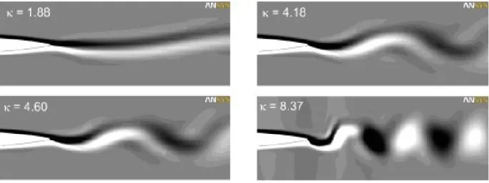
As previously mentioned, in most of the earlier works on elastic response of flexible bodies, the effects of fluid inertia or damping forces are often ignored. In the studies of Theodorsen (Theodorsen, 1935), Sears(Sears, 1941), and Garrick(Garrick, 1946) linear potential theory was used to obtain analytical expressions for the aerodynamic lift and moment of 2-D thin airfoils undergoing small amplitude oscillations in uniform inflow. Theodorsen’s (Theodorsen, 1935) approach assumed that: 1) the total lift force acts at the aerodynamic center (a quarter-chord downstream from the foil’s leading-edge; and 2) the wake behind the foil consists of shed vortices from the trailing-edge that convect downstream in a direction parallel to the inflow without any dissipation, at a fixed frequency. However, the real wake patterns shown in the studies of Anderson et al. (Anderson et al., 1998) and Munch et al.(Munch et al., 2010) are typically more complex than the wake patterns assumed in linear potential theory. The former author experimentally studied the wake patterns of a NACA0012 foil in a water tank for different flow regimes and observed a wavy wake without distinct vortices and with a very weak leading-edge vortex. Munch et al. (Munch et al., 2010) conducted numerical and experimental studies on a NACA0009 hydrofoil and showed that the pattern and strength of the wakes depend on the the reduced frequency of the oscillation motion, as depicted in Fig. 2.2.
Linear potential flow theory has been shown to be inadequate for modeling FSI problems with strong viscous effects. Connell and Yue (Connell and Yue, 2007) and Akcabay and Young (Akcabay and Young, 2012) numerically studied the dynamic response and stability
Figure 2.2 The wake pattern of a NACA0009 hydrofoil for four values of the reduced fre-quency, κ, (Munch et al., 2010)
of cantilever beams in viscous and axial flows. The latter authors validated their numerical results with several experimental data and showed that viscous effects are more significant for light beams in dense fluids due to the increased relative contribution of the fluid forces. They also found that fluid viscosity affects flutter of the structure, reduces the vibration amplitude, and changes the oscillation modes. More recently, Akcabay and Young (Akcabay and Young, 2014) compared their viscous simulation results with the predictions from the quasi-steady inviscid linear potential flow based theory. They concluded that the observed differences between results could be attributed to viscous effects, e.g. thickening of boundary layers, formation of trailing edge vortices, and flow separation. Considering the viscous effects, Ducoin and Young (Ducoin and Young, 2013) calculated the static divergence speed of a spanwise flexible cantilevered hydrofoil and showed that viscous effects help suppress or delay divergence.
The fluid damping and disturbing forces also depend on the flow velocity (Theodorsen, 1935; Sears, 1941; Liaghat, 2014). Reese (Reese, 2010) showed that the resonance frequencies and total loss factors of flexible hydrofoils depend on the flow velocity. This study involved hydrofoils made of relatively heavy and stiff materials for a limited range of flow velocity, and hence showed only a small dependence on the flow velocity.
In addition to the effects of velocity on the structural response, which is intuitively apparent, Reynolds number and angle of attack are also expected to affect the oscillations. Huang and Lin (Huang and Lin, 1995) and Jung and Park (Jung and Park, 2005) studied the unsteady characteristics of vortex shedding in the near wake of an oscillating foil for low Reynold numbers, Re ≤ 2.7 × 10⁴, and showed that the vortex shedding frequency varies with the
angle of incidence.
Boundary layer flows can be transitional around a lifting body at moderate Reynolds num-bers. The development of turbulent flow, which causes a momentum transfer normal to the wall, allows the flow to re-attach, and form a Laminar Separation Bubble (LSB). Flow separation, formation of trailing edge vortices, location and movement of the LSB affect the hydrodynamic loading and vibration of a flexible hydrofoil, which is the topic problem studied in this thesis. Hence, the precise prediction of the onset and the amount of flow separation plays a key role in the determination of the hydrodynamic loads on hydrofoils. Ducoin et al. (Ducoin et al., 2012a) experimentally investigated fluid structure interaction on a flexible hydrofoil in various flow regimes and concluded that the structural vibrations are induced by the laminar to turbulent boundary layer transition and depend on the vortex shedding frequency. Ducoin et al. (Ducoin et al., 2009a) showed that the LSB first appears near the trailing edge for low to moderate angles of attack, and as this is increased, it moves towards the leading edge. It was shown in the studies of Poirel et al. (Poirel et al., 2008) and Ducoin et al. (Ducoin et al., 2012b) that this movement of the LSB affects the hydrodynamic loading and vibration of a flexible hydrofoil. Poirel and Yuan (Poirel and Yuan, 2010) studied the laminar separation at transitional Reynolds numbers, 5.0 × 10⁴ ≤ Re ≤ 1.3 × 10⁵ and showed that the laminar separation can lead to flutter.
Summary
To recapitulate, the viscous effects, such as flow separation and vortices, have immediate effect on the hydrodynamic loads and response of hydrofoils. Furthermore, in the determination of hydroelastic response of flexible hydrofoils, it is crucial to precisely predict the onset and the amount of flow separation. This is particularly the case for high Reynolds number flows, in which the change of the wake pattern and vortex shedding frequency is substancially more noticeable. However, very limited studies are available for flexible hydrofoils at high Reynolds number flows.
In the present study, the hydroelastic response of hydrofoils subjected to moderate to high Reynolds number flows will be investigated.
2.3 Fluid-structure interaction
Fluid-structure interaction is a multiphysics phenomenon where the interaction between fluid flow and structural mechanics is taken into account. FSI is characterized by interactions, which can be stable or oscillatory, between a moving or deformable solid structure and a
surrounding or internal fluid flow. These effects cannot be neglected when evaluating the elastic response of lightweight flexible bodies due to the strong interplay between the body deformations and load distributions (Ward et al., 2018). This is a consequence of the high hydrodynamic load, which is proportional to the density of fluid. For instance, the density of water is approximately three orders of magnitude greater than that of air. Hence, a lifting body operating in water will experience much higher loads and resulting amplified FSI effects than a geometrically identical body in air at the same operating conditions (Harwood et al., 2016; Ward et al., 2018).
As evidenced from these studies, FSI problems play prominent roles in many engineering and scientific applications, yet, due to their strong nonlinearity and multidisciplinary nature, a comprehensive study of such problems remains a challenge (Hou et al., 2012). Different methods for the investigation of fluid–structure coupling have been extensively investigated (Tran et al., 2005; Dowell and Hall, 2001).
The FSI analyses can be generally categorized into two approaches; monolithic and parti-tioned methods. In monolithic approaches, both sub-fields (fluid and solid) are combined as one single problem. The non-linear, discrete system of equations resulting from the dis-cretization of the governing equations are solved as a whole (Barker and Cai, 2010; Gee, 2011). Ryzhakov et al. (Ryzhakov et al., 2010) presented a monolithic method for the simulation of the interaction between flexible structures and free surface flows and showed that their method was robust. However, this method leads to ill-conditioned system due to the different scaling of variables in the multi-field problem (velocity, displacement, pressure) (Ryzhakov et al., 2010) and might be very challenging to implement (Wu et al., 2015) and computationally expensive (Raja, 2012).
In contrast, the computational fluid dynamics (CFD) and computational structure dynamics (CSD) solvers can be coupled in a partitioned way. In this approach, which will be in-corporated in this study, the fluid and solid parts are solved using their distinct numerical methods. Interaction takes place regularly between the fluid and structure solvers via the coupling scheme which is based on successive solutions produced by the two solvers (Wu et al., 2015; Lefrançois, 2017). In an industrial context, the most important advantage that a partitioned approach offsets over a monolithic coupling approach (with a single solver) is the modularity of the coupling method, which makes the different solvers much easier to implement (Ryzhakov et al., 2010) and allows distributed computation (Lefrançois, 2017). Partitioned approaches can be categorized into two types: the loose coupling approach and the strong coupling approach. In a loosely coupled approach, only one single computation per time step is performed for each field (Lefrançois, 2017; Akcabay et al., 2017). Hence,
the coupling conditions at the interface may not be satisfied accurately (Sotiropoulos and Yang, 2014). Furthermore, loosely coupled (LC) partitioned FSI solvers suffer from numerical instabilities (Sotiropoulos and Yang, 2014), as each of the solid and fluid solvers can only use the other’s solution explicitly. This time-delay in the exchange of the boundary conditions (surface tractions and displacements) between the fluid and solid solvers can lead to errors, specially for FSI problems with lightweight structures in dense, incompressible flow (such as water); i.e. problems with low solid-to-fluid density ratios (Akcabay et al., 2017).
In order to avoid this numerical instability, strongly coupled partitioned algorithms with an iterative procedure are developed to improve the accuracy of the satisfaction of coupling conditions (Sotiropoulos and Yang, 2014; Lefrançois, 2017).
Two of the most common terms used when referring to the type of FSI analyses are one-way (unidirectional) and two-one-way (bidirectional). These terms reflect how the loads and displacements are transferred between the two domains. When fluid and solid are coupled by unidirectional load transfer, a given field may strongly affect, but not be affected significantly by the other field (Reference: ANSYS User Guide). When solving a one-way FSI problem, flow and structure are modeled within separate domains. The resultant loads from the flow field are then used to calculate the structural deflection (Liaghat et al., 2014), or the displacement of the structure can be used to update the boundary conditions and solve the flow field. In some Fluid-Structure Interaction simulations, however, there is a strong and potentially nonlinear relationship between the fields that are coupled. This is often the case in situations where the structure undergoes large amplitude deflections (Liaghat et al., 2014). Under these conditions, which is the case in many engineering applications, two-way FSI is required. Benra et al. (Benra et al., 2011) compared the one-way and two-way coupling methods for numerical analysis of fluid-structure interactions and showed that the results of two-way coupling methods were more accurate, especially for larger deflections where the fluid field is strongly influenced by structural deformation. They showed that a one-way coupling algorithm gives plausible results only for specific values in some cases, and does not guarantee energy conservation at the interface (Benra et al., 2011).
Matthies and Steindorf (Matthies and Steindorf, 2003) found that the weak coupling methods are explicit and hence, suffer from possible instabilities. They proposed a partitioned method to compute the transient response and showed that their method was faster, both in the number of iterations and in the overall numerical effort. In addition, it was shown to have superior convergence characteristics, and they concluded that strong coupling methods, where equilibrium is satisfied jointly between fluid and structure at each time step, are better suited. The hydroelastic coupling method of Young and Kinnas (Young and Kinnas, 2003a,b)
as-sumed small blade deformations. Applying Bernoulli’s equation, the total pressure was ex-pressed in terms of the rigid and elastic blade components, with the change in load stiffness and damping matrices. Coupling of the hydrodynamics with a structural analysis model to include the effect of blade vibration is described in (Young and Kinnas, 2004). Young (Young, 2007, 2008) analyzed time-dependent FSI of a propeller using a one-way approach by developing a 3-D potential-based boundary element method coupled with a 3-D finite el-ement method. Their predicted blade tip deflections, cavitation inception coefficient values, as well as cavitation patterns agreed well with experimental measurements.
Carstens et al. (Carstens et al., 2003) developed a coupled fluid-structure interaction algo-rithm to study the aeroelastic behaviour of vibrating blade assemblies. In their study, the motion of fluid and structure were integrated in time by separate time integration meth-ods while their interaction was accounted for through a coupling algorithm. However, to reduce the immense computational effort of a full-scale calculation, simplified structural and aerodynamic models were taken for the computations.
Moffatt and He (Moffatt and He, 2005) performed an evaluation on the use of coupled and decoupled methods for various turbomachinery applications. They predicted the resonant forced response of turbomachinery blades using a fully coupled approach and expected that, by combining the aerodynamic forcing and damping calculations in a single analysis, a higher computational efficiency would result compared to a classical uncoupled approach. Blade vibration in their coupled approach was modelled with a single degree-of-freedom (DoF) modal equation on the CFD mesh and solved simultaneously with the flow equations. The modal equation was solved and directly coupled with the flow equations at each solution step. Ducoin et al. (Ducoin et al., 2009b) incorporated a numerical one-way approach to analyze a deformable hydrofoil with transient pitching motion with a CFD finite volume code (CFX) for the fluid and a CSD finite element code (ANSYS) for the structure. Although there was good agreement with the experiments for the maximum displacement of the hydrofoil at low pitching velocities, for the highest pitching velocity, the simulation showed a stronger hysteresis effect than the experiment.
In the study of Munch et al. (Munch et al., 2010) a model was proposed to predict fluid–structure coupling by linearizing the hydrodynamic load acting on a rigid, oscillat-ing NACA0009 hydrofoil subjected to a turbulent, incompressible flow. The hydrofoil was modeled with forced and free pitching motions and the unsteady simulations of the flow were performed in ANSYS CFX and validated experimentally. Their proposed model could predict fluid–structure coupling with good precision when the response of the system was linearized. Their method was validated for limited values of the motion amplitude.
Ducoin and Young (Ducoin and Young, 2013) and Akcabay et al. (Akcabay et al., 2014) studied the hydroelastic response of two-dimensional flexible hydrofoils in viscous flows. Their numerical approach was based on a simple 2-DOF system (mass-spring-damper) to simulate the chordwise rigid hydrofoil which undergoes bend and twist deformations only, as shown in Fig. 2.3. In their study, the fluid and structure solvers were coupled using the Loose Hybrid Coupled (LHC) method presented in (Chae et al., 2013) and (Young et al., 2012). The LHC method is a partitioned FSI method, as it couples the solutions of the two separate fluid and structure solvers. The 2-DOF solid model in Refs. (Ducoin and Young, 2013) and (Akcabay et al., 2014) was used to calculate the hydrofoil motion at each time step. The fluid forces were extracted and applied on the 2-DOF model and solved for the new position of the hydrofoil within each time step. Ducoin and Young (Ducoin and Young, 2013) compared the predicted and measured lift coefficient and tip section displacement. Some discrepancies between experimental and numerical results were observed, which might be partly due to the 2-D flow assumption in their research, which ignored 3-D effects such as boundary layer effects, induced drag, and the use of a generalized 3-D structural model in their numerical framework. In their studies, LHC approach does not iterate within each time step and that is why the coupling between fluid and structure is loose in their simulations.
Figure 2.3 Dynamics of a 2D hydrofoil cross section with two DOF (Ducoin and Young, 2013)
Sotiropoulos and Yang (Sotiropoulos and Yang, 2014) presented an immersed boundary method to simulate complex fluid–structure interaction problems in engineering and biology. This method has emerged as a powerful numerical approach due to its inherent ability to han-dle arbitrarily complex domains with arbitrarily complex deformable immersed boundaries without the need for expensive and cumbersome dynamic re-meshing strategies or construct grids that conform to and deform with solid boundaries. However, a major disadvantage
of this method is the limitation in its ability to selectively cluster grid nodes in the vicin-ity of solid boundaries, which results in difficulties in simulations of high Reynolds number turbulent flows.
The major drawback of the classical partitioned FSI coupling scheme, according to (Lefrançois et al., 2016; Lefrançois, 2017), is that where the structure is surrounded by high density fluid there will be strong effects of added mass. Under this condition, convergence is not always guaranteed, or may be slow. Divergence will generally be observed, regardless of the chosen time step (Lefrançois, 2017). In 2016, Lefrançois et al. (Lefrançois et al., 2016) presented a numerical model for fluid-structure interactions in the context of sloshing effects in movable, partially filled tanks. The purpose of this model was to counteract the penalizing impact of the added mass effect on classical partitioned FSI coupling schemes. Results show that the corrected version systematically ensures convergence in cases where the classical FSI scheme fails to converge. In the rare cases where convergence was already obtained, the corrected version was shown to significantly reduce the number of required iterations.
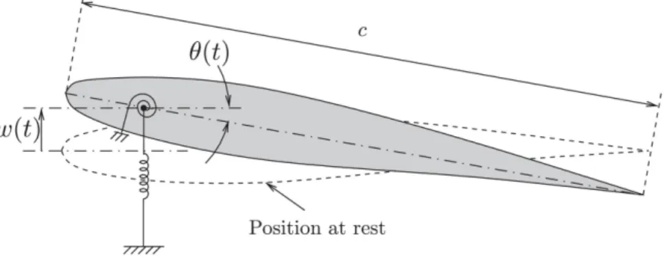
In 2017, Lefrançois (Lefrançois, 2017) presented a modified version of a partitioned FSI scheme for studying the dynamics of a NACA2412 foil flexibly attached and immersed in a heavy fluid. This work was based on an added mass corrected version of the classical strongly coupled partitioned scheme presented in (Song et al., 2013). The mathematical model for the structure in his study was limitted to the dynamics of a 2D foil that encountered only plunging and pitching motions (ω(t) and θ(t)), as shown in Fig. 2.4. Whereas the classical scheme encountered an acceptable (no numerical oscillation) convergence limit for fluid with certain density values, the corrected scheme in the study of Lefrançois (Lefrançois, 2017) was not dependent on fluid density.
Figure 2.4 A two-degrees-of-freedom model representing plunging and pitching (ω(t) and
θ(t)) of a 2D hydrofoil (Lefrançois, 2017)
of hydrofoils by comparing the inviscid and viscous fluid–structure interaction simulation of cantilevered NACA0015 hydrofoils in water. They studied hydrofoils made of stainless steel, aluminium and polyacetate (POM) under attached flow conditions in fully turbulent regimes at low angles of attack, and incorporated the LHC method presented in the studies of Young et al. (Young et al., 2012), Chae et al. (Chae et al., 2013), and Akcabay et al. (Akcabay et al., 2014). The 3D effects were neglected in their FSI method and it was recently applied by Wu et al. (Wu et al., 2018) to investigate transient characteristics of cavitating flow over a flexible 2D hydrofoil via combined experimental and numerical studies. The hydrofoil in theses studies was presented with a chord-wise rigid, two degree of freedom model and the pitching and plunging motion of the tip section was considered as the corresponding twisting and bending deformation of the hydrofoil.
Akcabay et al. (Akcabay et al., 2017) examined the numerical stability behavior of the LHC method, incorporated in (Young et al., 2012; Chae et al., 2013; Akcabay et al., 2014), to solve partitioned fluid and solid solvers for FSI problems. They showed that the LHC method is capable of stable solution to FSI problems, even for the difficult cases with small solid-to-fluid density ratios.
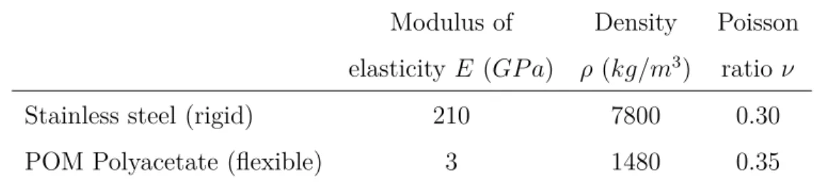
To the best of our knowledge, most of the former studies on the dynamic response of hydrofoils involved hydrofoils made of relatively heavy and stiff materials (Seeley et al., 2012; Liaghat et al., 2014; Yao et al., 2014; Liaghat, 2014). Hutchison (Hutchison, 2012) studied FSI for hydrofoils made of stainless steel (E=193 GP a, ρ=7750 kg/m3) and aluminium (E=71 GP a,
ρ=2770 kg/m3). The flexible hydrofoil in the study of Liaghat et al. (Liaghat et al., 2014; Liaghat, 2014) had a Young’s modulus of E=193 GP a and a density of ρ=8000 kg/m3. The increasing interest in the use of lightweight materials in the applications in which the solid-to-fluid density ratio is typically in the range of 1 and 2 (Chae et al., 2016), points to a better understanding of the elastic response and stability of lightweight lifting structures. These were investigated in Refs. (Ducoin and Young, 2013; Chae et al., 2013, 2016; Akcabay et al., 2014; Akcabay and Young, 2014).
Summary
Different methods for the solution of fluid-structure coupling have been extensively investi-gated in the literature. To study the hydroeastic behaviour of flexible hydrofoils, particularly at high hydrodynamic loadings, fluid and structure fields have strong and potentially nonlin-ear effects on each other. Hence, the solution method should be capable of strongly coupling and jointly satisfaction of equilibrium between fluid and structure. The two-way coupling method, which will be incorporated in the present study, is clearly required to tackle the large
structural deformations and subsequent effects on the flow fields, such as flow separation and instabilities. However, this method has not been recently used in this field. Recent increases in computer power coupled with advances in numerical methods, enable coupled two-way analyses of FSI in a reasonable time frame at an acceptable computational cost.
In addition, most of the hydrofoils studied in this field, have been made of relatively heavy and stiff materials. The present study will focus on highly flexible hydrofoils that undergo large deformation. As a consequence, the two-way FSI coupling is more challenging, particularly in the flow mesh deformation modelling.
2.4 Reasons for 3D simulation
In this dissertation, a two-way fluid-structure interaction (FSI) methodology is presented to study the hydroelastic response and stability of flexible hydrofoils with emphasis on three-dimensional features. This approach is validated by comparing the numerical results with measured experimental data by Akcabay et al. (Akcabay et al., 2014). To the best of our knowledge, despite the fact that the physics of the stated problem is 3D (as will be explained in what follows), most of the the previous studies on the hydroelastic response of hydrofoils have been restricted mainly to 2D simulations.
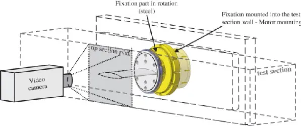
Experimentally and numerically, Chae et al. (Chae et al., 2016) investigated the natural flow-induced vibrations of flexible NACA0015 hydrofoils. The cantelivered hydrofoil in their study was clamped to the back wall of the test tunnel (foil root) and free to move on the other end of the test section wall (foil tip), as shown in Fig. 2.5. This set-up clearly illustrates the importance of 3D effects; i.e. the spanwise tip bending and twisting deformations of the flexible hydrofoil in their experiments. Due to these deformations, the hydrodynamic loading is not uniform in the spanwise direction. However, in their numerical simulation the flow was assumed to be two-dimesional.
The above mentioned cantilevered configuration of flexible hydrofoils have been studied in Refs. (Akcabay et al., 2014), (Akcabay and Young, 2014), (Ducoin and Young, 2013), (Wu et al., 2015), and (Chae et al., 2013). The hydrodynamic loading was assumed to be uniform over the spanwise direction in these studies. Despite the fact that the spanwise deformation will change the pressure distribution along that direction, they assumed that its effect on the foil deformation response is limited because of the small elastic deformation. However, for a flexible hydrofoil subjected to high flow velocities at high angles of attack, the elastic deformation is significant and cannot be neglected.
Figure 2.5 NACA0015 POM hydrofoil inside the tunnel (Chae et al., 2016)
such as bend and twist (as depicted in Fig. 2.5), the hydrodynamic loading is not uniform in the spanwise direction. For this reason, the interaction between hydrofoil and the sur-rounding flow has significant three-dimensional features that clearly should not be neglected. Furthermore, the flow is turbulent in the present study. It has been discussed in the previous sections that the flow separation and enhanced momentum exchange accompanied by the vortices induced by flow turbulence have a significant effect on the structural hydrodynamic response. Hence, the precise prediction of turbulence plays a key role in this area of research. It is widely accepted that turbulence is a three-dimensional phenomenon (Nichols, 2010). Turbulent disturbances can be considered as a series of three-dimensional eddies of different sizes that are in interaction with each other (Nichols, 2010). One important phenomenon in turbulent flows is vortex stretching. This is the lengthening of vortices in the flow, associ-ated with a corresponding increase of the component of vorticity in the stretching direction (Tennekes and Lumley, 1972). Vortex stretching is associated with a particular term in the vorticity dynamics equation:
D~ω
Dt = (~ω · ~∇)~v + ν∇
2ω (2.1)
where D/Dt is the material derivative, ~v is the velocity vector, ν is the fluid kinematic
viscosity and ∇2 is the Laplace operator. The first term on the right hand side describes the stretching or tilting of vorticity due to the flow velocity gradients. It amplifies the vorticity,
~
ω, when the velocity diverges in the direction parallel to ~ω. This term has been shown to be
zero in 2D formulation, and hence, 3D simulations are necessary to capture this important feature of turbulence.
Summary
The hydroelastic deformation of hydrofoil has significant 3D features that will be accounted for in the present study. Particularly, in the case of highly flexible hydrofoils which undergo large deformation, the 3D effects should not be neglected for the accurate prediction of the hydrodynamic loading. Furthermore, for proper investigation of turbulent flows and the 3D turbulence structures, which have immediate effects on the response of flexible hydrofoils, 3D simulation is a necessity. However, most of the the previous studies on the hydroelastic response of hydrofoils have focused mainly on 2D simulations.
2.5 Objectives
This project seeks to gain greater insight into the hydroelastic response of a 3D highly flexible hydrofoil, incorporating a strongly-coupled two-way fluid-structure interaction. The fluid-structure problem in the present study is solved with a finite volume technique using the CFD code CFX, for the fluid, and a finite element code using the CSD code ANSYS, for the structure.
As discussed in the preceeding literature review, the elastic response and stability of lifting bodies have been studied extensively in the literature. However, to the best of our knowledge, most of the studies are limited to no or small viscous effects, low Reynolds number flows, and low structural deformation due to the low material flexibility. Furthermore, in the numerical studies of hydrofoils, most of the analyses have focused on 2D problems with weak or no FSI. Accordingly, the objectives of the project are outlined as follows:
• To develop an advanced methodology to investigate the strongly-coupled two-way FSI of a 3D flexible hydrofoil with a focus on the in-water response,
• To improve the accuracy of the available numerical results for the lift and drag coeffi-cients in comparison with the available experimental data,
• To investigate and quantify the foil flexibility effects by studying the differences in struc-tural response as well as hydrodynamic loading (fluid response) between a lightweight, highly flexible hydrofoil and a rigid hydrofoil,
• To investigate the hydrodynamic response of a hydrofoil subject to different flow regimes at moderate to high Reynolds numbers.
CHAPTER 3 THEORETICAL BACKGROUND
The solution of FSI problems involves the simulation of the fluid and solid domains and their interaction. In the present study, we will focus on the interaction between an incompressible flow and a flexible hydrofoil. This area inherits all the difficulties of the 3D turbulent flow simulation in hydrodynamics, and complements them with the ones related to the strong FSI coupling, such as moving boundaries and large mesh deformation. There are various numerical techniques to tackle this kind of problems, some of which will be elaborated on in this chapter. In the study of FSI, which is a complex combination of CFD and CSD, it is essential to understand the basic physical principles and governing equations of these fields. These will be addressed in the present chapter.
3.1 Numerical modeling of Fluid-structure interaction
FSI modeling consists in performing a structural analysis coupled to a corresponding fluid flow analysis. There are two different approaches for solving such problems, the monolithic approach and the partitioned approach, which are described below.
3.1.1 Monolithic approach
In monolithic approaches a single, non-linear, discrete system of equations is considered taking into account both the fluid and the structure domains simultaneously, as described in (Barker and Cai, 2010; Gee, 2011). Figure 3.1 represents the solution process of such an approach in which Sf and Ss denote the fluid and structure solutions, respectively. t
n and
tn+1 represent the nth and n + 1th time steps.
Figure 3.1 Monolithic approach (Raja, 2012)
The interaction between fluid and structure at the interface is treated synchronously in this approach. This leads to the conservation of properties at the interface, which increases the stability of the solution. However, as explained in the previous chapter, this expensive
approach is complicated to implement and leads to ill-conditioned systems due to the different scaling of variables in the multi-field problem (velocity, displacement, pressure).
3.1.2 Partitioned approach
In the partitioned methods, the equations governing the flow field and the structure are solved alternatingly in time with two distinct solvers. The intermediate flow solution is prescribed as a boundary condition to update the structure and vice versa, and the iterations continue until a convergence criterion is satisfied. Figure 3.2 illustrates the solution process in a partitioned approach. The exchange of information occurs at the fluid-structure interface based on the type of coupling technique applied; i.e. one-way or two-way coupling methods that will be described in the following sections.
Figure 3.2 Partitioned approach (Raja, 2012)
One-way coupling
In a one-way FSI analysis, the CFD results are transferred and applied as loads to the me-chanical model, but the subsequently calculated displacements from the meme-chanical analysis are not transferred back to the CFD analysis. The other way around is also possible, i.e. the deformation of structure influences the flow field but the reaction of the fluid upon the solid object is negligible.
As illustrated in Fig. 3.3, in a one-way coupling method, initially, the fluid flow calculation is performed until convergence is reached. Then, the resulting forces at the interface from the fluid calculations are interpolated onto the solid computational domain. Next, the struc-tural dynamic calculations are performed until the convergence criterion is reached. This is repeated until the final time of the simulation is reached.