Synchronous Machine Modeling Precision and Efficiency in Electromagnetic Transients

UNIVERSITÉ DE MONTRÉAL

SYNCHRONOUS MACHINE MODELING PRECISION AND EFFICIENCY IN ELECTROMAGNETIC TRANSIENTS

ULAS KARAAGAC

DÉPARTEMENT DE GÉNIE ÉLECTRIQUE ÉCOLE POLYTECHNIQUE DE MONTRÉAL

THÈSE PRÉSENTÉE EN VUE DE L’OBTENTION DU DIPLÔME DE PHILOSOPHIAE DOCTOR (Ph.D.)

(GÉNIE ÉLECTRIQUE) NOVEMBRE 2011

UNIVERSITÉ DE MONTRÉAL

ÉCOLE POLYTECHNIQUE DE MONTRÉAL

Cette thèse intitulée

SYNCHRONOUS MACHINE MODELING PRECISION AND EFFICIENCY IN ELECTROMAGNETIC TRANSIENTS

présentée par : KARAAGAC Ulas

en vue de l’obtention du diplôme de : Philosophiae Doctor a été dûment acceptée par le jury d’examen constitué de :

M. KOCAR Ilhan, Ph.D., président

M. MAHSEREDJIAN Jean, Ph.D., membre et directeur de recherche M. GAGNON Richard, Ph.D., membre

ACKNOWLEDGEMENTS

I would like to express my deepest gratitude to my supervisor Prof. Jean Mahseredjian for his guidance, encouragement, patience, support and especially friendship. His innovative and questioning approach, his broad knowledge and his real life experience in Power Systems discipline helped me to establish a solid understanding and vision. I learned a lot from him about how to think different and to be creative. I think this is the most important asset that one can gain from a Ph.D. program.

Special thanks goes to colleagues working in Planning Department of Turkish Transmission Company for providing practical cases used in this study.

Greatest appreciation is reserved for my wife, Asli for her patience, support and encouragement.

Finally, I would like to express special thanks to my parents Yunus and Kezban for their endless love and support.

RÉSUMÉ

L’objectif principal de cette thèse est l’élaboration d’une méthode de modélisation de la machine synchrone plus performante et plus précise, et des algorithmes pour le calcul et la solution des transitoires électromagnétiques. Le pas d’intégration numérique est un facteur clef pour ces aspects. La possibilité d’utiliser des pas plus grands permet d'augmenter la vitesse des calculs et donc d'étendre le champ d'application des méthodes de type électromagnétique.

Cette thèse propose quatre modèles de façon à améliorer la précision du modèle dq0 classique tout en maintenant son efficacité. Trois de ces modèles utilisent le dq0 avec une précision accrue de la modélisation. Parmi les modèles précis se retrouve le dq0 avec des pas d'intégration intermédiaires. L’efficacité est maintenue par la restriction du modèle à l’usage durant des intervalles transitoires, là où la précision du modèle classique dq0 diminue. Ces modèles fournissent une modélisation précise tout en maintenant la vitesse du dq0 classique. Cependant, ils sont conçus spécialement pour les cas typiques d'étude de stabilité transitoire de réseau, et leur précision se détériore quand l’exactitude du modèle est nécessaire pour une grande partie de l’intervalle de simulation complète. Le meilleur modèle nommé PD-dq0 est obtenu en appliquant la transformation de ‘’Park’’ aux équations discrétisées dans le domaine des phase.

Les études d’évaluation de la précision et de l’efficacité démontrent que le modèle PD-dq0 est supérieur aux autres modèles proposés dans la littérature.

L’analyse de précision est effectuée avec les contraintes de précision du réseau environnant. Donc, ce travail contribue également à une meilleure évaluation de la précision numérique et de l’efficacité des engins de simulation étudiés.

La thèse se termine par des analyses au niveau des méthodes d'implémentation des équations de machine synchrone dans les équations de réseau et des solveurs de matrices

creuses. Les analyses permettent de déduire des améliorations de performance numérique selon les choix de modèle et de solution par matrices creuses.

ABSTRACT

The main objective of this dissertation is the establishment of more efficient and more precise synchronous machine modeling approaches and solution algorithms for the computation of electromagnetic transients (EMT). Numerical integration time step size is a key factor in both aspects. The capability to use larger time steps in EMT-type simulation methods also contributes to the extension of such methods into the efficient simulation of electromechanical transients.

In this thesis, four new models are proposed in order to improve the precision of the classical dq0 model while maintaining its efficiency. Three of them use the classical dq0 model with increased accuracy. The most accurate models are: dq0 with internal intermediate time step usage, phase-domain and voltage behind reactance. Efficiency is maintained by restricting the accurate model usage to the transient intervals where the precision of the classical dq0 formulation decreases. This approach provides accuracy while maintaining classical dq0 computational speed. However, these three models are designed for typical transient stability cases and their performance deteriorates when the accurate model usage is needed for a large portion of the complete simulation interval. The last forth model proposed in this thesis is obtained by applying Park’s transformation to the discretized equations of the phase-domain model. This model maintains the precision of the phase-domain model and eliminates its computational inefficiencies through a constant admittance matrix. Unlike the first three models, its efficiency does not change with simulated system and phenomenon. Precision and efficiency assessment studies demonstrate that this model is superior in both aspects and should be chosen for the computation of both electromagnetic and electromechanical transients in the same computational framework.

The models proposed in this thesis are compared for practical cases and conditions. Precision analysis is performed within the accuracy constraints of the surrounding network and numerical efficiency assessment analysis accounts for the utilized sparse

matrix solver and refactorization scheme. Hence, this work also contributes to better assessment of both numerical precision and efficiency for researched machine models in this thesis and in the recent literature.

This thesis also proposes two new synchronous machine representations for Modified-Augmented-Nodal-Analysis (MANA) formulation. In the first formulation, a machine Thevenin equivalent equation is inserted directly into the main network equations (MNE) using MANA. The second representation is proposed for phase-domain and voltage behind reactance models. In this representation all machine equations are inserted into the MNEs, thus eliminating the requirement of interfacing circuits. Although these formulations do not improve simulation speed, they demonstrate the modeling flexibility achievable through MANA and allow to verify performance hypothesis based on partial factorization.

LIST OF FIGURES ... xiii 

LIST of NOTATION and ABBREVIATIONS ... xvi 

CHAPTER 1. ... 1 

INTRODUCTION ... 1 

1.1.  Background ... 3 

1.1.1.  Power System Network Equations in EMTP-type Programs ... 3 

1.1.2.  Synchronous Machine Modeling in EMT-Type Programs ... 5 

1.2.  Motivation ... 7 

1.3.  Methodology ... 10 

1.4.  Summary of Results and Contributions ... 12 

1.5.  About this Thesis ... 18 

CHAPTER 2. ... 19 

SYNCHRONOUS MACHINE EQUATIONS ... 19 

2.1.  Basic Equations for Electrical Part ... 19 

2.2.  Park Transformation ... 23 

2.3.  Voltage-Behind-Reactance (VBR) Formulation ... 28 

2.4.  Magnetic Saturation ... 32 

2.4.1.  dq0 Model Equations with Magnetic Saturation ... 36 

2.4.2.  PD Model Equations with Magnetic Saturation... 37 

2.4.3.  VBR Model Equations with Magnetic Saturation ... 38 

2.5.  Basic Equations for Mechanical Part ... 40 

DISCRETE-TIME SYNCHRONOUS MACHINE MODELS AND SOLUTION

PROCEDURES IN EMT-TYPE PROGRAMS ... 42 

3.1.  Discrete-Time Mechanical Part Model ... 43 

3.2.  Discrete-Time dq0 Model ... 44 

3.3.  Discrete-Time PD Model ... 51 

3.4.  Discrete-Time VBR Model ... 55 

3.5.  Discrete-Time dq0 Model with Internal Intermediate Time Step Usage (dq0-IITS Model) ... 60 

3.6.  Combinations of dq0 Model with PD and VBR Models (dq+PD and dq+VBR Models) ... 68 

3.7.  Discrete Time PD-dq0 Model ... 70 

CHAPTER 4. ... 75 

STUDIES FOR NUMERICAL PRECISION – EMTP-RV SIMULATIONS ... 75 

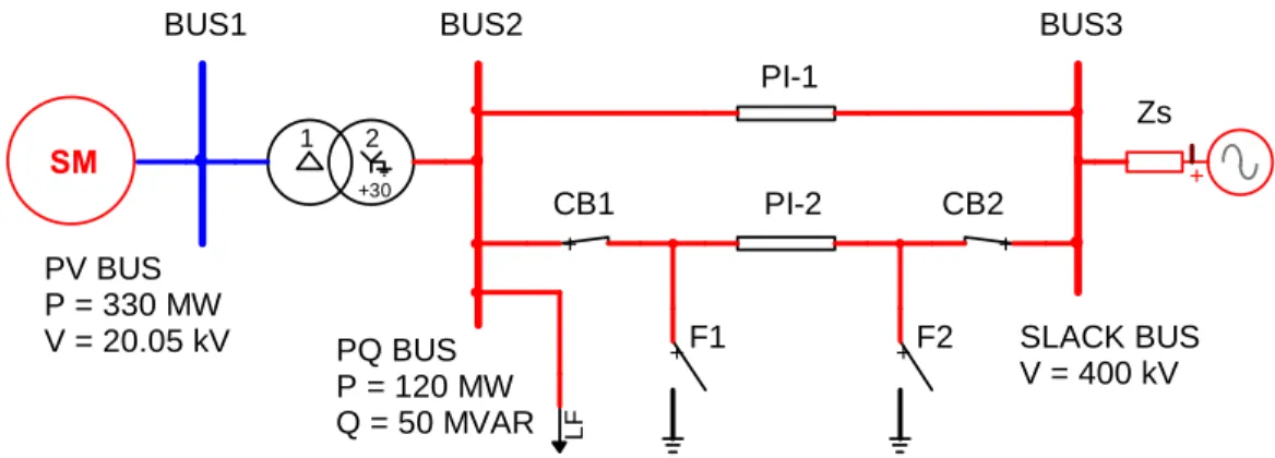
4.1.  Single Machine - Infinite Bus System ... 76 

4.1.1.  Test Case C1 ... 77  4.1.2.  Test Case C2 ... 84  4.1.3.  Test Case C3 ... 86  4.1.4.  Test Case C4 ... 88  4.1.5.  Test Case C5 ... 90  4.1.6.  Test Case C6 ... 91 

4.2.  Transient Stability Case ... 93 

4.2.1.  System Description ... 93 

4.2.2.  Simulated Cases ... 96 

4.2.3.  Simulation Results ... 96 

4.3.  Subsynchronous Resonance (SSR) Case ... 101 

4.3.1.  System Description and Simulated Cases ... 101 

4.3.2.  Simulation Results ... 103 

COMPLEMENTARY STUDIES FOR NUMERICAL EFFICIENCY ASSESSMENT

... 107 

5.1.  Background on Modified Augmented Nodal Analysis (MANA) Formulation 108  5.1.1.  MANA Formulation with Machine Thevenin Equivalents (MANA-Thevenin) ... 109 

5.1.2.  MANA Formulation with Machine Complete Electrical Equations (MANA-Complete) ... 110 

5.2.  Solution of Main Network Equations ... 115 

5.3.  Partial Refactorization ... 116  5.4.  MatEMTP Simulations ... 119  CHAPTER 6. ... 127  CONCLUSIONS ... 127  REFERENCES ... 131  Appendix I ... 136 

Input Data Conversion ... 136 

Appendix II ... 147 

Linear Predictors ... 147 

Appendix III ... 149 

Aλ, BI, Bλk, bVF, Kλ(ω), KI, Kλk(ω), Kpλk and kVF in Discrete-Time VBR Machine Model ... 149 

Appendix IV ... 152 

LIST OF TABLES

Table 4.1 Single Machine - Infinite Bus Cases ... 77 

Table 4.2 Error e%, Armature Currents, Test Case C1 ... 77 

Table 4.3 Error e%, Armature Currents, Test Case C1 ... 79 

Table 4.4 Error e%, Armature Currents, Test Case C1 (0 to 0.22 s only) ... 81 

Table 4.5 Error e%, Electrical Torque, Test Case C1 ... 84 

Table 4.6 Error e%, Armature Currents, Test Case C2 ... 85 

Table 4.7 Error e%, Electrical Torque, Test Case C2 ... 86 

Table 4.8 Error e%, Armature Currents, Test Case C3 ... 86 

Table 4.9 Error e%, Electrical Torque, Test Case C3 ... 86 

Table 4.10 Error e%, Armature Currents, Test Case C4 ... 90 

Table 4.11 Error e%, Electrical Torque, Test Case C4 ... 90 

Table 4.12 Error e%, Armature Currents, Test Case C5 ... 90 

Table 4.13 Error e%, Electrical Torque, Test Case C5 ... 91 

Table 4.14 Error e%, Armature Currents, Test Case C6 ... 93 

Table 4.15 Error e%, Electrical Torque, Test Case C6 ... 93 

Table 4.16 Power Injections, Total Load and Network Losses ... 95 

Table 4.17 Circuit Breaker Fault Clearing Times ... 95 

Table 4.18 Error e%, Electrical Torque, TS-C1 ... 97 

Table 4.19 Error e%, Electrical Torque, TS-C2 ... 97 

Table 4.20 Error e%, Electrical Torque, TS-C1 (with Damping Resistor Usage) ... 98 

Table 4.21 CPU Timings in pu based on dq0 model, TS-C1 ... 99 

Table 4.22 SSR System Model Summary ... 101 

Table 4.23 SSR Cases ... 101 

Table 4.24 Error e%, Electrical Torque, SSR-C1... 103 

Table 4.25 Error e%, Electrical Torque, SSR-C2... 103 

Table 4.26 Error e%, Electrical Torque, SSR-C3... 103 

Table 4.27 Error e%, Electrical Torque, SSR-C4... 103 

Table 5.1 Simulation Codes, Utilized Machine Models, Sparse Matrix Solvers,

MANA Refactorization Schemes ... 120 

Table 5.2 Detailed CPU Timings in EMTP-RV Simulation ... 120 

Table 5.3 Detailed CPU Timings in MatEMTP Simulations ... 121 

Table 5.4 Ordering Quality Comparison ... 123 

Table 5.5 Expected CPU Timings in EMTP-RV Simulation with KLU usage (based on MatEMTP simulations) ... 124 

Table 5.6 Expected CPU Timings in EMTP-RV Simulation with Partial Refactorization Scheme (based on MatEMTP simulations) ... 124 

Table 5.7 Expected CPU Timings in EMTP-RV Simulation with partial refactorization scheme, KLU and MNA-Thevenin usage (based on MatEMTP simulations) ... 126 

Table 5.8 Expected CPU Timings in EMTP-RV Simulation with partial refactorization scheme, KLU and MNA-Complete usage (based on MatEMTP simulations) ... 126 

Table I.1 Transient and Subtransient Inductances and Time Constants ... 144 

Table I.2 Equivalent Data Sets ... 144 

LIST OF FIGURES

Figure 2.1 Stator and rotor circuits of a synchronous machine ... 19 

Figure 2.2 Synchronous machine with rotating armature windings ... 25 

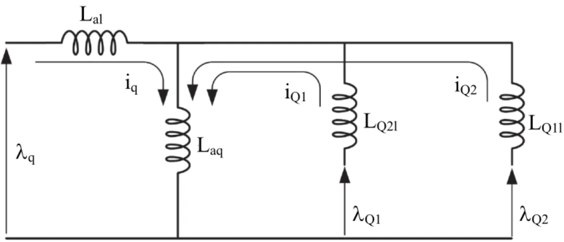
Figure 2.3 d -axis equivalent circuit illustrating flux-current relationship ... 26 

Figure 2.4 q -axis equivalent circuit illustrating flux-current relationship ... 27 

Figure 2.5 Saturated and unsaturated mutual fluxes ... 34 

Figure 2.6 Magnetic saturation characteristic (piecewise-linear approximation) ... 34 

Figure 2.7 Structure of a typical lumped multimass system ... 40 

Figure 3.1 Solution following a discontinuity... 42 

Figure 3.2 Linear three-point prediction with smoothing ... 47 

Figure 3.3 Solution algorithm for dq0-IITS model ... 67 

Figure 3.4 Solution algorithm for dq0-PD model ... 69 

Figure 4.1 Single line diagram of the simple single-machine system... 76 

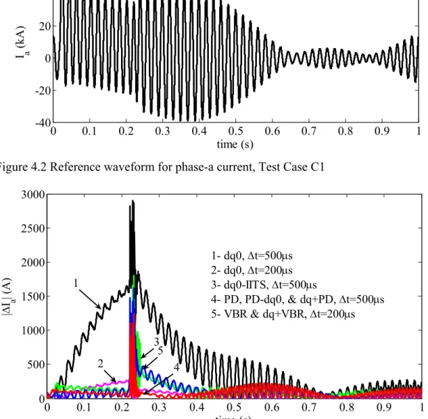
Figure 4.2 Reference waveform for phase-a current, Test Case C1 ... 78 

Figure 4.3 Differences between the numerical solutions and the reference waveform for phase-a currents, Test Case C1 ... 78 

Figure 4.4 Accurate model usage period in dq0-IITS, dq+PD and dq+VBR models, Test Case C1 ... 80 

Figure 4.5 Phase-a currents during fault removal, Test Case C1 ... 80 

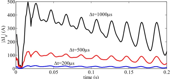
Figure 4.6 Time delay in switch opening due to large time step usage, Test Case C1 .... 81 

Figure 4.7 The effect of utilized time step on simulation starting transient, Test Case C1, PD-dq0 model ... 83 

Figure 4.8 Reference waveform for electrical torque, Test Case C1 ... 83 

Figure 4.9 Differences between the numerical solutions and the reference waveform for electrical torque, Test Case C1... 84 

Figure 4.10 Differences between the numerical solutions and the reference waveform for phase-a currents, Test Case C2 ... 85 

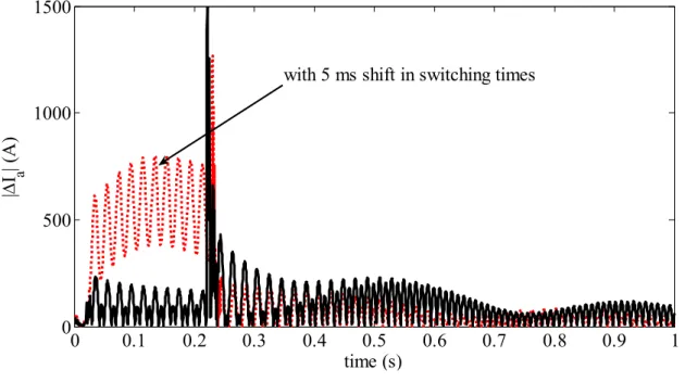
Figure 4.11 Effect of 5 ms shift in switching times on phase-a current (reference waveform) in Test Case C3 ... 87  Figure 4.12 Effect of 5 ms shift in switching times on the difference between the numerical solution and the reference waveform of phase-a current for dq0 model with

500

t s

  in Test Case C3 ... 87  Figure 4.13 Effect of 5 ms shift in switching times on dq0 model armature current errors in Test Case C3 ... 88  Figure 4.14 Differences between phase-a currents and the reference waveform for Test Cases C1 and C4, PD-dq0 model,  t 500s ... 89  Figure 4.15 Jump in machine operating conditions due to operating segment change in the saturation curve ... 89  Figure 4.16 Differences between phase-a currents and the reference waveform for Test Cases C1 and C5, PD-dq0 model,  t 200s ... 91  Figure 4.17 Numerical solutions with PD-dq0 model and the reference waveform for phase-c current on transformer magnetizing branch, Test Case C6,... 92  Figure 4.18 Zoomed version of Figure 4.17 ... 92  Figure 4.19 Differences between phase-a currents and the reference waveform for Test Cases C5 and C6, PD-dq0 model,  t 200s ... 93  Figure 4.20 Single line EMTP-RV diagram of the transient stability case ... 94  Figure 4.21 Simplified single line diagram of the BORCKA Substation ... 96  Figure 4.22 Field currents (pu) for the synchronous machines of Figure 4.20, TS-C1 ... 98  Figure 4.23 Single line EMTP-RV diagram of the SSR case ... 102  Figure 4.24 Machine terminal voltages (pu) for the synchronous machines in HAMIT, KEBAN and KANGA; SSR-C2 ... 105  Figure 4.25 Machine field currents (pu) for the synchronous machines in HAMIT, KEBAN and KANGA; SSR-C2 ... 105  Figure 5.1 MNE coefficient matrix (number of non-zeros = 2187) ... 122  Figure 5.2 Block triangular form of MNE coefficient matrix (number of non-zeros = 2187) ... 122 

Figure 5.3 Continuously refactorized matrix in partial refactorization scheme (A_n22,

number of non-zeros = 783) ... 125 

Figure I.1. d -axis equivalent circuit representing the complete characteristic ... 136 

Figure I.2. q -axis equivalent circuit representing the complete characteristic ... 137 

LIST of NOTATION and ABBREVIATIONS

(1.1) Equation 1.1

[1] Reference 1

n

A Linear Augmented Network Matrix in MANA formulation n

b Vector of known currents and voltages in MANA formulation m

D Tridiagonal matrix of damping coefficients dq0

i Vector of stator currents in dq0 variables n

i Vector of current sources in NA formulation r

i Vector of rotor currents s

i Vector of stator currents in phase variables m

J Diagonal matrix of moments of inertia m

K Tridiagonal matrix of stiffness coefficients L Lower triangular matrix

 

L Subtransient inductance matrix dq0rs

L Rotor-stator inductance after Park’s transformation dq0sr

L Stator-rotor inductance after Park’s transformation dq0ss

L Stator-stator inductance after Park’s transformation rr L Rotor-rotor inductance

 

 

 

λ Vector of stator flux linkages in dq0 variables r

λ Vector of rotor flux linkages s

p _{d dt /}

P Number of poles

 

P Park’s transformation matrix C

P Column permutation matrix R

P Row permutation matrix

R Scaling matrix

r

R Diagonal rotor resistance matrix s

R Diagonal stator resistance matrix a

T Vector of torques

mach

T Electromagnetic torque of the machine

 Angle between magnetic d-axis and magnetic phase a-axis in electrical rad

m

θ Vector of angular positions in rad u Vector of speed voltages

U Upper triangular matrix 

abc

v Vector of subtransient voltages dq0

v Vector of stator voltages in dq0 variables n

v Vector of node voltages in NA formulation r

v Vector of rotor voltages s

v Vector of stator voltages in phase variables  Rotor angular speed, in electrical rad/s

m

ω Vector of speeds in rad n

x Vector of unknown currents and voltages in MNA formulation n

AMD Approximate Minimum Degree ATP Alternative Transient Programs BTF Block Triangular Factorization

COLAMD Column Approximate Minimum Degree CPU Central Processing Unit

EBA Backward Euler Integration Method EMT

EMTP

Electromagnetic Transients

Electromagnetic Transients Program

EMTP-RV Electromagnetic Transients Program Restructured Version FACT Flexible AC Transmission

HPP Hydraulic Power Plant

HVDC High-Voltage Direct-Current IITS Internal Intermediate Time Step MatEMTP Transient Analysis Program in MATLAB M-files MANA

MNA

Modified-Augmented-Nodal-Analysis Modified Nodal Analysis

MNE Main Network Equations MMD Multiple Minimum Degree

NA Nodal Analysis

NE Norton Equivalent

PD Phase-Domain

SSR Subsynchronous Resonance

TE Thevenin Equivalent

TPP Thermal Power Plant

TRAP Trapezoidal Integration Method VBR Voltage-Behind-Reactance

CHAPTER 1.

INTRODUCTION

Simulation of electromagnetic transients in modern power systems is widely used for the determination of component ratings such as insulation levels and energy absorption capabilities, in the design and optimization process, for testing control and protection systems and for analyzing power system performance in general [1], [2]. In order to simulate electromagnetic transients, various simulation tools have been developed. These simulation tools are called EMTP-type programs and can be categorized as nodal (or modified-nodal or modified-augmented-nodal) equation based and state variable (state-space) based simulators. Contrary to nodal equations, the automatic formulation of state-space equations is significantly more time consuming and requires the computation of the network topological proper-tree. Large scale system simulation software packages are based on nodal equations. The list of packages (EMT or EMTP type programs) includes: EMTP-RV [3], EMTP96 [4], ATP/EMTP [5] and PSCAD/EMTDC [6]. EMTP96 was abandoned after the development of EMTP-RV. ATP is based on the original code of EMTP [4] which evolved to become EMTP96. EMTP-RV is a more recent software and the only one using MANA formulation. The SimPowerSystems software included in the Simulink environment uses state-space formulation [7].

Due to the increased in speed of modern computers and recent improvements in numerical methods, EMT type programs can now be used for studying transient stability (electromechanical transients) or even small signal stability problems, although such studies are traditionally performed using transient stability (stability-type) programs [1], [2]. In transient stability programs, the energy exchange between generators and other dynamic equipments is assumed to take place while the electric network is remaining at system frequency (quasi-steady state approach using fundamental frequency

representation), i.e. the electromagnetic transients are totally ignored during computation of electromechanical transients. This assumption enables the utilization of large simulation time steps (typically 1 to 8 ms for 60 Hz systems), hence provides much better computational speeds when compared to EMT type programs. On the other hand, the stability type method assumptions may lead to significantly inaccurate simulation results. In addition, the fundamental frequency phasor modeling techniques can not directly represent the faster transients characterizing the power electronic based equipments such as HVDC and FACTS components. Therefore, the EMT type programs are becoming indispensable also for simulating electromechanical transients in power systems.

Synchronous machines are essential components in all power systems. They form the principle source of electric energy and provide reactive power required by the transmission network. Moreover, many large industrial loads are driven by synchronous machines. Therefore, accurate modeling and simulation of synchronous machines is indispensable in EMTP type programs. Numerous machine models and solution procedures have been proposed in the literature. Although these models are based on the lumped-parameter coupled electric circuit approach and remain equivalent in continuous time domain, the numerical properties of these models differ when their equations are discretized by utilizing a particular integration method. Hence, the machine models and solution procedures have significant influence on simulation precision and speed. Moreover, depending on the simulated phenomenon and the system model, the machine model or its solution procedure might become a limiting factor that imposes very small integration time steps and causes reduced simulation speeds.

This dissertation presents new modeling approaches and solution procedures for synchronous machines in the computation of electromagnetic transients. The proposed modeling approaches and solution procedures improve computational efficiency significantly while maintaining precision. In addition to simple infinite bus analysis, the proposed modeling approaches and solution procedures are also compared for more

sophisticated and practical cases. This dissertation also studies sparse matrix solver and refactorization schemes in relation with machine models. Computational speed remains the main target in all studies.

1.1. Background

1.1.1. Power System Network Equations in EMTP-type Programs The nodal equation based power system network model has been widely used in EMTP-type programs. The main system of symmetric equations for an n node system is given by

n n n

Y v = i (1.1)

Equation (1.1) is referred to as the standard nodal analysis (NA) formulation in the literature and it is based on the assumption that the admittance matrix model exists for all network components. In (1.1), Y_n is the admittance matrix, v_n is the vector of node voltages and i_n is the vector of current sources combined with history current sources for the trapezoidal integration method. Since there are usually voltage sources (known node voltages) in the simulated power system model, (1.1) must be partitioned to keep only the unknown voltages on the left hand side

    n n n s s

Y v = i Y v (1.2)

In (1.2), Y_n is related only to unknown node voltages v_n, i_n holds the sum of currents entering nodes with unknown voltage, and Y_sY_n relates to known voltages v_s. It should be noted that v = v_n





The assumption of admittance model existence for every component is a significant limitation. (1.2) becomes a variable rank system to model the ideal switch operations which reduce the computational efficiency, especially when the number of switches and switching frequency become high. In addition, direct representation of the branch relations and the devices with voltage and current relations is not possible. These limitations can be eliminated by using Modified-Augmented-Nodal-Analysis (MANA) formulation as introduced in [9] and improved in [10] and [11]. In MANA formulation, (1.1) is augmented to include extra generic equations and the system of network equations becomes

n n n

A x = b (1.3)

In (1.3), x_n contains the unknown voltage and current quantities, b_n contains the known current and voltage quantities and A_n is the linear augmented network matrix (Y_nA_n).

For generic power systems, both Y_n in (1.2) and A_n in (1.3) are sparse. Therefore, depending on used formulation in EMTP type program, the solution of (1.2) or (1.3) is obtained using sparse matrix methods and LU factorization [12]. It is common to use special ordering techniques to obtain sparser LU factors for better solution speed. A_n in (1.3) has a larger size compared to Y_n in (1.2); however, using (1.3) instead of (1.2) does not cause a significant increase in simulation speed due to utilization of efficient sparse matrix solvers. As MANA formulation in (1.3) is superior over NA and MNA, this thesis considers MANA formulation.

Throughout this thesis the system of network equations given in (1.2) and (1.3) will be referred as main network equations (MNE); Y_n in (1.2) and A_n in (1.3) will be referred as MNE coefficient matrices.

1.1.2. Synchronous Machine Modeling in EMT-Type Programs

In EMT-type programs, synchronous machines are modeled outside of the power system network and require a special interface in both NA and MANA formulations. Depending on the utilized machine model, the methods of interfacing machine models with the power system network can be classified into indirect and direct approaches [13].

1.1.2.1. Indirect Approaches

In indirect approaches, the classical dq0 model [14] for synchronous machine is interfaced with the power system network expressed in physical variables and phase coordinates. There are currently three different approaches used to interface the dq0-model of the machine with the power system network.

In the first approach [15], the machine is interfaced using a Norton equivalent in phase coordinates. The Norton resistance matrix is approximated to become time-independent and the Norton current sources result from predicted machine electrical and mechanical variables. Synchronous machine models SM module in EMTP-RV, Type-59 in EMTP96 (also ATP), fall into this category. In EMTP-RV it is optionally possible to iterate with MNE to achieve voltage convergence.

The second approach [16] is based on the compensation method in which the main network is represented as a Thevenin equivalent circuit and interfaced with the synchronous machine dq0 circuits. The universal machine model in ATP/EMTP is implemented using this method. The compensation method suffers, however, from topological limitations [17] and is not considered in this thesis.

In the third approach, used in PSCAD/EMTDC, the machine model is interfaced with the main network as a compensation current source and a special terminating resistance [18]. The Norton current source, that represents the machine, is calculated

using the previous time point terminal voltages of the machine. Hence one time-step delay exists in this approach and this approach is not considered in this thesis.

The key advantage of the first approach over the direct methods is utilization of constant admittance matrix at the expense of predicting certain electrical variables. This eliminates the time consuming refactoring of the MNE coefficient matrix at each solution time point and increases simulation speed. However, accumulation of prediction errors may cause numerical noise problems (in some cases) and even instability especially with large time steps. In order to improve the model stability, it is common to use damping resistances in parallel with model circuit inductances at the expense of reduced model accuracy [15], [19], [20], [21]. However, as illustrated in [21] and in this thesis, the error due to damping resistances is less noticeable at large time steps due to reduced overall accuracy.

1.1.2.2. Direct Approaches

The phase-domain (PD) model is in the original form of the coupled electric circuit in which the model is expressed in physical variables and phase coordinates [22], [23]. In this model, the machine circuits are directly inserted into the MNE, thus providing a simultaneous solution. It has been demonstrated that this approach improves numerical accuracy and stability [24]-[27]. However, due to the time variant self and mutual inductances of the PD model, it is required to update and refactor the MNE coefficient matrix at each solution time point at an increased computational cost. Type-58 in ATP/EMTP is implemented using this model [28].

The voltage-behind-reactance (VBR) machine model was introduced in [29] for the state variable approach and extended to nodal analysis in [26]. As in the PD model, the stator circuit is expressed in phase coordinates and directly inserted into the MNE in order to achieve a simultaneous solution. On the other hand, the rotor equations are expressed in dq-rotor reference. In [26] the analysis of PD and VBR models concludes that the VBR model has a better numerical accuracy and a lower computational cost

when compared to the PD model. However, as in the PD model, due to the time variant self and mutual inductances of the VBR model, it is needed to update and refactor the MNE coefficient matrix at each solution time point.

1.2. Motivation

Although numerous machine models and solution procedures have been proposed for EMTP type programs, their effect on simulation accuracy and speed has not been investigated in details. Analysis for the accuracy assessment of the machine models and solution methods have been presented in [26] for balanced and in [27] for unbalanced faults. In both studies, the accuracy of numerous machine models and solution methods are compared for various numerical integration time step size usage in order to make overall simulation efficiency evaluation. The numerical integration time step size is a key factor in both aspects. On the other hand, in both studies, the accuracy assessment is performed based on the results of machine terminal fault simulations in a simple single-machine infinite bus system which includes only the fault period. In normal practice, it is necessary to simulate faults on transmission facilities. Moreover, the system simulation should also include the fault removal and continue until stability assessment becomes possible. As the presented results in [26] and [27] totally ignore the effect of reduced precision in the surrounding network due to large time step usage, these results are not sufficient to conclude on modeling performance. Therefore, a better assessment of numerical precision for researched machine models is required.

While studying electromechanical transients, such as transient stability or subsynchronous resonance, it is needed to model a large portion of the targeted power system since electromechanical transients include frequency perturbations. Depending on the power system model, the poor accuracy of classical dq0 model might force the utilization of a small numerical integration time step. This creates significant computing time problems for large scale cases and repetitive simulations. However, it can be shown that as the time step increases, the classical dq0 model introduces significant errors

especially in the DC component of armature currents following a discontinuity (fault condition) in the power network. For these types of studies, the simulation accuracy can be improved by switching to a more accurate model (PD or VBR) or a more accurate dq0 model solution procedure following a large disturbance in the network and switching back to classical dq0 model as the DC component of armature currents decays to small values. The more accurate solution for dq0 model can be obtained by implementing an internal intermediate (fractional) time step usage between two existing MNE solution time points at the expense of reduced simulation speed resulting from solving the machine equations more than once. For typical transients, the accurate model or solution procedure is expected to become active only for a small portion of the complete simulation interval. Hence this solution approach is expected to provide similar simulation accuracy with the accurate model or solution procedure while maintaining classical dq0 model like simulation speed.

Although all dq0, PD and VBR models are based on lumped-parameter coupled electric circuit approach and equivalent in continuous time domain, the numerical properties of these models differ when their equations are discretized. The inaccurate behavior of dq0 model at large time steps is resulting from its discretized equations. Therefore, the dq0 model can be reformulated by applying Park’s transformation to the discretized equations of the PD model to maintain PD model like accuracy. By implementing a prediction-correction scheme, constant machine admittance matrix usage in MNE can be achieved to provide classical dq0 model like computation efficiency.

Unlike the classical dq0 model, the PD and VBR models need to update and refactor the MNE coefficient matrix at each solution time point. The increase in simulation time due to the usage of the PD model instead of the classical dq0 model is investigated in [24]. In this study, the simulation times are compared for the classical dq0 and PD models usage in ATP (Type-59 and Type-58 synchronous machine models, respectively) for the same time step usage. It should be noted that, ATP performs

complete refactorization at each solution time point. However, the increase in simulation time due to usage of PD or VBR models is expected to be affected by implemented refactorization schemes. In addition, the effect of the sparse matrix solver efficiency on simulation speed is expected to be different for PD and VBR models due to their refactorization requirements at each solution time point. Therefore, the comparisons between the models that use constant and time-varying MNE coefficient matrices should be done by considering these facts. On the other hand, partial refactorization schemes may create other matrix ordering problems and such schemes have not been tested and proven for large scale practical systems.

In both NA and MANA formulations, the machines are represented in MNE by modifying Y_n and i_n with their Norton equivalent circuits. On the other hand, MANA formulation does not require or force the admittance model usage. Power system network models in the MANA formulation can be augmented to include extra generic equations based on the machine equations and the nodal relations where the machine is connected. For example inserting Thevenin equivalent circuits of the machines into the MNE will eliminate the calculation of Norton equivalent circuits of the machines at each time step. With this formulation, the solution of the MNE will provide the machine stator currents in addition to the machine stator voltages; hence the calculation of machine stator currents following MNE solution will be also eliminated. When all machine electrical circuit equations are inserted into the MNE, the calculations to form the machine interfacing circuit for the MNE solution and the calculations to find machine electrical variables following the MNE solution will be completely eliminated. It should be noted that, such MANA formulations will increase the size of the MNE coefficient matrix, hence the MNE solution time. However, the increase in the MNE solution time might be less when compared to the time gained from the computations regarding machine equations, especially for efficient sparse matrix solvers.

1.3. Methodology

The methodology used in this thesis is to start by implementing the classical dq0, PD and VBR models. This work is followed by research on new solutions algorithms and modeling approaches. All models are implemented and tested through user-defined modeling facilities available in EMTP-RV [10]. In addition to simple single machine - infinite bus test cases, the machine model performances are also compared for actual practical and large scale cases. In all cases, precision analysis includes surrounding network constraints.

In all simulations, the reference solutions for precision comparisons are obtained from the contributed EMTP-RV software implementation of the PD model and 1 s simulation time step (t) [21]. It should be noted that in all simulated cases, all models converge to the reference solution with smaller simulation time step usage and the differences between the reference solutions become negligible for  t 1s. The simulations are repeated for all models for different simulation time steps from 50 s _to 1ms . In order to evaluate the accuracy of different numerical solutions, the relative

error between the reference solution trajectory ( f ) and the given numerical solution ( f ) is calculated using the 2-norm [30]:

2 2

e% f f f (1.4)

Simulation accuracy is directly related to the utilized machine model; hence EMTP-RV simulations are sufficient to conclude on model accuracy. On the other hand, as the MNE coefficient matrix is constant for indirect approaches and time-varying for direct approaches, the effect of the sparse matrix solver and implemented refactorization schemes on computational efficiency is different for these approaches. Therefore, EMTP-RV simulations are not sufficient to conclude on the computational efficiency of these models.

For a reasonable computational efficiency comparisons, PD, VBR and the most accurate and efficient models proposed in this thesis are implemented in MatEMTP (a transient analysis program in MATLAB M-files) [9] in addition to proposed MANA formulations and partial refactorization scheme. Three different sparse matrix solvers are used in MatEMTP in order to demonstrate its effect on simulation efficiency. These sparse matrix solvers are:

 LU factorization with approximate column minimum degree ordering (COLAMD) [31],[32];

 LU factorization with approximate minimum degree ordering (AMD) [33],[34];  KLU Matrix-solve package [35].

All simulations are performed on a computer having a four-core CPU of 2.67 GHz and 4G RAM. Model computational efficiency evaluation is done based on the CPU timings of a practical case simulation. In order to correlate MatEMTP with EMTP-RV CPU timings, the total simulation time (t_sim) is decomposed as follows

&

sim ss update A b refactor MNE solve MNE comp

t t t _ t _ t _ t (1.5)

where

 t_ss: the CPU time for steady state solution, system component initialization and preparation for time-domain simulation,

 t_{update A b &} : the CPU time for updating A_n and b_n in (1.3),  t_{refactor MNE} : the CPU time for refactoring A_n in (1.3),

 t_{solve MNE} : the CPU time for solving factorized version of (1.3),

 t_comp: the CPU time for updating network equivalents of each system component for MNE solution and solving their equations following MNE solution.

The reasoning behind the decomposition of t_sim into five parts is for correctly accounting for their different shares in total simulation time of EMTP-RV and

MatEMTP. Any conclusion made based on only the changes in total simulation time of MatEMTP will not be valid for EMTP-RV. Therefore, the changes in t_{update A b &} ,

refactor MNE

t _ , t_{solve MNE} and t_comp in MatEMTP simulations are considered separately to estimate the possible EMTP-RV simulation times with the proposed MANA formulations, partial refactorization scheme for PD and VBR models, and different sparse matrix solver packages.

1.4. Summary of Results and Contributions

The overall contributions and results of this thesis are summarized below:

1. Assessment of Numerical Precision for Existing Machine Models: Unlike existing studies ([26] and [27]), the existing and proposed machine models are compared for more practical cases and conditions. Simulation results show that for a given simulation time step, PD or VBR model usage provides much better precision compared to the classical dq0 model. However, their usage instead of the classical dq0 model does not provide the improvement stated in [26] in practical cases due to the following reasons:

 For a given simulation time step, the classical dq0 model produces less error during fault conditions for the faults on transmission facilities compared to the faults at machine terminals due to large impedance between the fault and the machine terminals,

 Large time step usage causes reduced accuracy in the surrounding network solution and consequently the precisions for all models,

 Large time steps usage create initialization errors and discrepancies with the steady-state phasor solution. This obvious observation is reconfirmed to avoid erroneous statements made in some papers.

According to simulation results, PD and VBR models have similar precision for a given simulation time step. In some cases, they enable utilizing twice the time step of the classical dq0 model while maintaining simulation precision.

2. Discrete-Time dq0 Model with Internal Intermediate Time Step Usage (dq0-IITS): The classical dq0 model solution algorithm is modified by implementing an option for internal intermediate (fractional) time step usage between two existing main network solution time points. This approach improves precision at the expense of reduced simulation speed resulting from solving the machine equations more than once. However, internal intermediate time step usage is restricted to the transient intervals where the precision of the dq0 formulation decreases. As demonstrated in this thesis, when simulation time step is increased, the classical dq0 model introduces significant errors especially in the DC component of armature currents following a fault condition. The restriction of internal intermediate time step usage is achieved by implementing a network switching detection and machine terminal voltage monitoring algorithm for the startup of the transient (perturbation) interval and a field current monitoring algorithm for the decision process of moving back to normal time step after the perturbation interval. For a typical transient stability case, internal intermediate time step usage becomes active only for a small portion of the complete simulation interval. In addition, electromagnetic transients are local by nature, which limits the number of machines with intermediate time point solutions while simulating large scale systems. Therefore, the increase in simulation time is not significant. This solution approach provides similar accuracy with the PD and VBR models.

Similar to the classical dq0 model, this model may require damping resistances for some cases and for larger time-steps, but even with damping resistances it is still able to provide accuracy comparable to PD and VBR models and especially for balanced faults. It should be also noted that, the error due to damping resistances is less noticeable at large time steps due to reduced overall accuracy.

3. Combinations of Classical dq0 Model with PD and VBR Models (dq+PD and dq+VBR): The combinations of the classical dq0 approach with PD and VBR models are designed to improve the performances of the PD and VBR models respectively. Similar to dq0-IITS, the objective is to restrict the usage of PD or VBR modeling to the transient intervals where the precision of the classical dq0 formulation decreases while maintaining dq0 throughout the rest of the simulation. This is achieved by implementing network switching detection and a machine terminal voltage monitoring algorithm for the startup of the transient (perturbation) interval and a field current monitoring algorithm for the decision process of moving back to dq0 after the perturbation interval. For typical transient stability cases, this approach is as precise as the accurate PD and VBR models while maintaining classical dq0 model like simulation speed.

In the dq+PD and dq+VBR models, damping resistances are present only when the machines are using the classical dq0 model. It should be noted that, damping resistances produce high errors during fault conditions due to high armature currents. The effect of damping resistances on the accuracy of the dq+PD and dq+VBR models is not significant because these models move into the PD and VBR models respectively during fault duration.

4. Discrete Time PD-dq0 Model: Although the mathematical backgrounds of classical dq0 and PD models are equivalent in continuous time domain, the numerical properties of these models differ when their equations are discretized. As demonstrated in [21] and in this thesis, the inaccurate behavior of the classical dq0 model at larger time steps is related to its discretized equations. To combine the accuracy of the PD model with the efficiency of the dq0 model, this model is obtained by applying Park’s transformation to the discretized equations of the PD model. As it emanates from the discretized PD model, it delivers an accuracy similar to the PD model. As for the classical dq0 model, a prediction-correction scheme is implemented for interfacing with MNE through a constant admittance matrix for computational efficiency. In short, this

model inherits precision and performance from the PD and dq0 models respectively. It is the best model delivered in this thesis.

Alike the classical dq0 model the PD-dq0 version may require damping resistances for correcting numerical stability problems in some cases with large time step usage. However, the error due to damping resistances is less noticeable at large time steps due to reduced overall accuracy.

The driving idea in the dq0-IITS, dq+PD and dq+VBR models is the usage of accurate models for the time intervals where the precision of the classical dq0 formulation decreases. These models are designed for typical transient stability cases where accurate model usage is needed for a small portion of the complete simulation interval. Depending on the simulated phenomenon and the surrounding system model, computational speeds of these models may deteriorate. Therefore, the PD-dq0 model is superior over the proposed dq0-IITS, dq+PD and dq+VBR models.

Although implementing partial refactorization scheme improves the computational efficiency of PD and VBR models significantly, their computational performance is still poor compared to the PD-dq0 model. Therefore, the PD-dq0 model is also superior over the existing machine models in the literature due to its high precision and computational performance. In addition, it offers the advantage of programming simplicity in existing classical dq0 model codes in EMT type programs.

5. Assessment of Numerical Efficiency for Machine Models: PD and VBR models are much less efficient due to time consuming updating and refactoring of the MNE coefficient matrix. In EMTP-RV, PD and VBR models require more than twice the computational time compared to the classical dq0 model for a given simulation time step. Hence, PD or VBR model usage does not provide any advantage in EMTP-RV while simulating practical cases. However, EMTP-RV uses a complete refactorization

scheme and a sparse matrix solver that employs multiple minimum degree ordering (MMD) to obtain sparser LU factors [3]. In this thesis the implementation of partial

refactorization is demonstrated for various sparse matrix solvers and tested in MatEMTP for a practical case including several synchronous machines. Partial refactorization reduces MNE solution time by 38.7% in MatEMTP simulations for both PD and VBR model usage when LU factorization is used with AMD. By considering this improvement in MatEMTP, total simulation time in EMTP-RV is expected to reduce by 27.7% and 28.5% for PD and VBR model usage, respectively. With this improvement, both PD and VBR models become superior to the classical dq0 model due to their better precision. On the other hand, their computational performance is still very poor compared to the proposed PD-dq0 model.

It should be noted that large simulation time step usage is correlated with the simulated network model. For example, using more precise propagation delay based models for transmission lines instead of multi-phase pi-section models, impose a hard upper limit on simulation time step. Moreover, the usage of large simulation time steps may cause convergence problems in the iterative process with nonlinear devices or other drifts in precision. In such cases, not only the proposed PD-dq0 model, but also the classical dq0 model may be preferred due to its high computational efficiency if it provides acceptable precision.

This thesis also investigates the impact of the utilized sparse matrix solver on simulation efficiency for a typical EMT-type solution method. The machine models using constant and time-varying MNE coefficient matrices, partial and complete refactorization schemes are taken into account. The KLU sparse matrix solver provides the most efficient simulations in all cases, as expected. The improvement in simulation speed with the KLU sparse matrix solver usage instead of LU factorization with AMD, reduce the MNE solution time by 86.4% in MatEMTP simulations with the PD-dq0 model. By considering this improvement in MatEMTP, total simulation time of EMTP-RV is projected to reduce by 25.9%. On the other hand, the improvement in the MNE solution time with KLU usage is smaller in MatEMTP for PD and VBR models with partial refactorization schemes (around 43.5%). This improvement in MatEMTP implies

around 17.2% and 16.5% expected decrease in total simulation time of EMTP-RV for PD and VBR models, respectively. Although, KLU usage improves the simulation speed for all models, the computational difference between PD-dq0 and VBR (or PD) models is expected to become more significant in a typical EMT-type program.

6. Alternative Machine Representation in MNA: As MANA formulation does not require the admittance model for power system components; it enables different machine representations in the MNE. This thesis proposes two new machine representations in MANA formulation. In the first formulation, the Thevenin equivalents of the machines are inserted into the MNE to eliminate machine Norton equivalent calculations and machine stator current calculations following the MNE solution. In the second formulation, all machine equations are inserted into the MNE to eliminate interfacing circuit calculations and machine electrical variable calculations following the MNE solution. It should be noted that, this formulation introduces time dependent terms in the MNE coefficient matrix for the PD-dq0 model. As the advantage of constant MNE coefficient matrix usage disappears, this formulation is not suitable for the PD-dq0 model; hence it is proposed only for PD and VBR representations.

The above formulations are tested in MatEMTP with the KLU sparse matrix solver usage and partial refactorization scheme for PD and VBR models. The first formulation decreases the total simulation time of MatEMTP by 2.6%, 6.0% and 5.3% for PD-dq0, VBR and PD models respectively. However, detailed analysis shows that the possible decrease in EMTP-RV simulation time will be 1.5% for PD-dq0 and below 1% for both PD and VBR models with this formulation. The second formulation decreases the total simulation time of MatEMTP by 20.9% and 18.3% for VBR and PD models respectively. On the other hand, detailed analysis shows that this formulation may even reduce simulation efficiency when transposed into EMTP-RV.

Although proposed formulations are not expected to improve the efficiency of an EMT-type program, they demonstrate the flexibility of MANA.

1.5. About this Thesis

The work presented in this thesis is divided into following chapters:

 Chapter I, Introduction: Motivation, study methodology and important contributions are presented following a brief presentation of EMT-type programs and synchronous machine modelling approaches in the computation of electromagnetic transients.  Chapter II: Synchronous Machine Equations: Mathematical modeling of the

synchronous machine is presented in details.

 Chapter III: Discrete Time Synchronous Machine Models and Solution Procedures in EMTP-Type Programs: The proposed new synchronous machine models and solution procedures for the computation of electromagnetic transients are presented in addition to the existing models and solution procedures in the literature.

 Chapter IV: Studies for Numerical Precision – EMTP-RV Simulations: EMTP-RV simulation results are presented to compare both the precision and efficiency of the proposed models and the existing models in the literature.

 Chapter V: Complementary Studies for Numerical Efficiency Assessment: Partial refactorization implementation and proposed MANA formulations are presented for the direct machine modeling approaches. MatEMTP simulation results are presented for a reasonable efficiency comparison between direct and indirect modeling approaches that considers refactorization scheme, MANA formulation and applied sparse matrix solver.

CHAPTER 2.

SYNCHRONOUS MACHINE EQUATIONS

2.1. Basic Equations for Electrical Part

Figure 2.1 Stator and rotor circuits of a synchronous machine

Figure 2.1 illustrates the circuits involved in the analysis of a synchronous machine. The stator circuits are composed of three-phase armature windings and the rotor circuits are composed of the field and the damper windings. Although a large number of circuits are used to represent damper effects in machine design analysis, a limited number of circuits may be used in power system analysis depending on the type of rotor construction and the frequency range of interest. Usually the damper effects are represented with three damper windings: one located on d-axis, and other two located

on q -axis [36]. The rotor circuits have therefore three damper windings and the mathematical model of the machine is based on this assumption in this thesis.

In Figure 2.1, a, b and c are the stator phase windings; F is the field winding, D is the d-axis damper winding; Q₁ and Q₂ are the first and second q -axis damper windings;  is the angle between magnetic d-axis and magnetic phase a-axis in electrical rad;  is the rotor angular speed in electrical rad/s.

It should be noted that the electrical equations for one pole-pair machine are the same with the machines having more than one pole-pair except the rotor angular speed and the torque calculated for the mechanical part. The necessary conversion can be done as follows:









where P is the number of poles; _mach and T_mach are the actual angular speed and electromagnetic torque values;  and T are the angular speed and electromagnetic torque values for the 2-pole machine.

The following assumptions are made while developing the mathematical model of the synchronous machine [36]:

 The mmf in the air-gap has sinusoidal distribution and the space harmonics are neglected.

 The effect of stator slots on the rotor inductances is neglected; i.e., saliency is restricted to the rotor.

 The magnetic hysteresis is neglected.

The omission of magnetic saturation effects is made to deal with linear coupled circuits and make superposition applicable in the derivation of the basic equations of the synchronous machine. However, saturation effects can be significant and the necessary corrections for accounting their effects will be discussed in Section 2.4.

The stator and rotor flux linkages can be written as

 

 

_{ }

 

The vectors i_{s and} λ_{s denote the stator currents and flux linkages; the vectors} i_r and λ_{r denote the rotor currents and flux linkages.} L_ss

 

 

 

Stator-Stator Inductances: The variation of the permeance of magnetic flux path

with the rotor position produces the second harmonic terms for both self and mutual inductances. The stator self and mutual inductances can be expressed as [36]:

 

 

























cos 2 cos 2 2 3 cos 2 2 3

cos 2 2 3 cos 2 2 3 cos 2

cos 2 2 3 cos 2 cos 2 2 3

aa ab ab ab aa ab ab ab aa aa L L L L L L L L L L                                    _   _        s ss s L L (2.4)

where L_aa0 and L_ab0 correspond to the constant part of the self inductance of each stator winding and mutual inductance between any two stator windings, respectively. L_aa2 is the maximum value of the second harmonic term for both the self inductance of each stator winding and the mutual inductance between any two stator windings.

Stator-Rotor Inductances: The variation of the mutual inductance is due to the relative motions of the windings. The stator-rotor mutual inductances can be expressed as

 

1 2

1 2

1 2

cos cos sin sin

2 2 2 2

cos cos sin sin

3 3 3 3

2 2 2 2

cos cos sin sin

3 3 3 3 aF aD aQ aQ aF aD aQ aQ aF aD aQ aQ L L L L L L L L L L L L                                    _{ }  _{ }  _{ }  _{ }  _                    _{   }           _{       }   sr L (2.5) where L_aF, L_aD, L_aQ1, L_aQ2 are the maximum values of the mutual inductances

between stator phase windings (a,b,c) and the F , D , Q1, Q2 windings, respectively.

Rotor-Stator Inductances: As L_ij L_ji for i a b c , , and jF D Q Q, , ₁, ₂, the rotor-stator mutual inductances can be expressed as

 

 

L L (2.6)

Rotor-Rotor Inductances: The self inductances of the rotor circuit and the mutual

inductances between each other do not change with the rotor position. The constant rotor-rotor inductance matrix can be written as

1 1 1 2 1 2 2 2 0 0 0 0 0 0 0 0 FF FD FD DD Q Q Q Q Q Q Q Q L L L L L L L L                rr L (2.7)

where L_FF , L_DD, L_{Q Q1 1} and L_{Q Q2 2} are the self inductances of the windings F , D , Q₁

and Q₂, respectively. L_FD is the mutual inductance between _{F and D windings;} L_{Q Q1 2}

The voltage equations for the stator and rotor windings are p                         s s s s r r r r v R 0 i λ = - -v 0 R i λ (2.8)

The vector v_s denotes the stator voltages and the vector v_r denotes the rotor voltages. It should be noted that, only the field voltage v_F in v_r is non-zero. R_s and

r

R are constant diagonal matrices containing the stator and rotor resistances, i.e.









where r_a, r_F, r_D, r and _Q1 r are the resistances of the stator, F , D , _Q2 Q1 and Q2

windings, respectively.

Generator convention is used while expressing the voltage equations; that is, the currents are assumed to be leaving the winding at the terminals and the terminal voltages are assumed to be the voltage drops in the direction of currents. The electromagnetic torque expression can be found from the co-energy function as below [36]:

 

 

2.2. Park Transformation

Equations (2.3), (2.8) and (2.11) completely describe the electrical behavior of the synchronous machine. However, these equations can be solved numerically and they are not suitable for analytical solution due to time varying inductances. The time-invariant set of machine equations can be obtained through Park Transformation [14]. The new fictitious quantities are obtained from the projection of the actual stator variables along

three axes, which are the direct axis of the rotor winding (d axis), quadrature axis ( q

-axis) and the stationary axis. In other words, all the stator quantities are transformed into new fictitious (dq0) variables in which the reference frame rotates with the rotor. Thus, by definition

 

s dq0

f P f (2.12)

where f_s are the stator phase quantities that can be either voltages, currents or flux linkages of the stator windings and f_dq0 are new fictitious quantities. The park transformation matrix P

 

 

















The constants k_d, k and _q k₀ are arbitrary and their values may be chosen to simplify the numerical coefficients in performance equations. Power invariant transformation (i.e., P

 

 

2 3

q

k  and k0  1 3 [36]. The major advantage of this transformation is that, all

the transformed mutual inductances are reciprocal. The flux linkages in terms of dq0 variables are given by

                          dq0ss dq0sr dq0 dq0 dq0 dq0 dq0rs rr r r r L L λ i i = L L L λ i i (2.14)

Here the vectors i_dqo and λ_dqo denote the stator currents and flux linkages in dq0 variables respectively. The inductance matrix L_dq0 is constant due to Park’s transformation and given by

 

   





 

 

 

 

   



 

 



It should be noted that, the fictitious d winding is aligned with the d -axis and the fictitious q winding is aligned with the q -axis as illustrated in Figure 2.2. Hence, there is no coupling between the fictitious d ( q ) winding and the rotor windings on q ( d )-axis.