UMR CNRS 7024
ANNALES DU LAMSADE N°7
Mai 2007
Robustness in OR-DA
Guest Editors: Bernard Roy, Mohamed Ali Aloulou, Rim Kalaï
Numéro publié grâce au Bonus Qualité Recherche accordé par l’Université Paris IX - Dauphine Responsables de la collection : Vangelis PASCHOS, Bernard ROY
Comité de Rédaction : Cristina BAZGAN, Marie-José BLIN, Denis BOUYSSOU, Albert DAVID, Marie-Hélène HUGONNARD-ROCHE, Eric JACQUET- LAGRÈZE, Patrice MOREAUX, Pierre TOLLA, Alexis TSOUKIÁS.
Pour se procurer l’ouvrage, contacter Mme D. François tél. 01 44 05 42 87 e-mail : [email protected]
I La collection « Cahiers, Documents et Notes » du LAMSADE publie, en anglais ou en français, des travaux effectués par les chercheurs du laboratoire éventuellement en collaboration avec des chercheurs externes. Ces textes peuvent ensuite être soumis pour publication dans des revues internationales. Si un texte publié dans la collection a fait l'objet d'une communication à un congrès, ceci doit être alors mentionné. La collection est animée par un comité de rédaction.
Toute proposition de cahier de recherche est soumise au comité de rédaction qui la transmet à des relecteurs anonymes. Les documents et notes de recherche sont également transmis au comité de rédaction, mais ils sont publiés sans relecture. Pour toute publication dans la collection, les opinions émises n'engagent que les auteurs de la publication.
Depuis mars 2002, les cahiers, documents et notes de recherche sont en ligne. Les numéros antérieurs à mars 2002 peuvent être consultés à la Bibliothèque du LAMSADE ou être demandés directement à leurs auteurs.
Deux éditions « papier » par an, intitulées « Annales du LAMSADE » sont prévues. Elles peuvent être thématiques ou représentatives de travaux récents effectués au laboratoire.
COLLECTION "CAHIERS, DOCUMENTS ET NOTES" OF LAMSADE The collection “Cahiers, Documents et Notes” of LAMSADE publishes, in English or in French, research works performed by the Laboratory research staff, possibly in collaboration with external researchers. Such papers can (and we encourage to) be submitted for publication in international scientific journals. In the case one of the texts submitted to the collection has already been presented in a conference, it has to be mentioned. The collection is coordinated by an editorial board.
Any submission to be published as “cahier” of LAMSADE, is sent to the editorial board and is refereed by one or two anonymous referees. The “notes” and “documents” are also submitted to the editorial board, but they are published without refereeing process. For any publication in the collection, the authors are the unique responsible for the opinions expressed.
Since March 2002, the collection is on-line. Old volumes (before March 2002) can be found at the LAMSADE library or can be asked directly to the authors.
Two paper volumes, called “Annals of LAMSADE” are planned per year. They can be thematic or representative of the research recently performed in the laboratory.
III
Éditorial
Les contributions qui constituent le présent volume ont, pour la plupart d’entre elles, donné lieu à présentations orales et débats au sein d’un groupe de travail. Ce groupe, créé en 2003 par Bernard Roy sous l’égide du LAMSADE, avait pour objet de confronter, de comparer et d’approfondir les travaux de recherche ayant trait à la robustesse en recherche opérationnelle et aide à la décision, lesquels devenaient de plus en plus nombreux et diversifiés. Deux réunions d’une journée entière se sont tenues chaque année. Chacune d’elles a rassemblé des chercheurs et enseignants-chercheurs provenant d’universités multiples, essentiellement françaises et belges. Ce groupe de travail a bénéficié d’un soutien dans le cadre du programme de coopé-ration entre le CNRS et le FNRS/CGRI Belgique.
Tous les articles de ce volume ont été soumis, sous le contrôle des éditeurs, à une procédure d’arbitrage mobilisant, pour chacun, deux arbitres. Dans le présent vo-lume, les articles ont été rangés par ordre alphabétique du premier auteur. Toutefois, pour les présenter brièvement, nous avons adopté ci-après un critère de rangement différent qui nous a conduits à les regrouper en quatre familles.
La première rassemble deux articles qui, chacun à leur manière, visent à mettre en évi-dence l’intérêt du sujet dont traite le présent volume ainsi que la variété des travaux qui lui sont consacrés dans la littérature. Il s’agit des articles de L. Dias et B. Roy.
L’article de L. Dias débute par une rapide présentation des difficultés les plus cou-rantes auxquelles le chercheur opérationnel se heurte pour attribuer une valeur aux paramètres que comportent les modèles d’aide à la décision (décision individuelle ou de groupe). L’analyse de robustesse a pour objet de répondre à ces difficultés. L’auteur décrit trois usages possibles qui mettent en évidence les bénéfices que l’on peut retirer de « l’outil analyse de robustesse » en les faisant intervenir du début à la fin du processus de décision. VIP analysis et IRIS lui servent d’exemples pour illus-trer ses propos. L’auteur met l’accent sur la recherche de conclusions robustes plutôt que sur celle de solutions robustes. Il souligne ainsi le rôle de la modélisation comme processus constructif d’apprentissage.
Après avoir défini le sens qu’il attribue au qualificatif « robuste » (en RO-AD), B. Roy explique pourquoi il préfère parler de « préoccupation de robustesse » plutôt que d’analyse de robustesse. Il explicite et approfondit ensuite les multiples raisons d’être de cette préoccupation. Afin de mieux mettre en évidence le caractère multi facettes de cette préoccupation, il propose de regarder les travaux traitant de robus-tesse en les situant sur trois versants : les deux premiers, qualifiés respectivement de
standard (S) et concret (C), présentent des traits caractéristiques qui les opposent à
bien des égards alors que le troisième, mixte (M), est destiné à supporter ceux des travaux qui ne présentent que trop imparfaitement tous les traits caractéristiques requis pour pouvoir être clairement affectés à l'un des deux versants précédents. Dans la section 4, il montre que, sur chacun de ces trois versants, la préoccupation de robustesse devrait produire des formes de réponses encore plus variées qu’elles
IV Les trois autres familles dont il va être question maintenant rassemblent ceux des articles qui se situent successivement sur les versants standard, mixte et concret. Six articles se situent clairement sur le versant standard S. Il s’agit des articles de H. Aïssi, C. Bazgan, D. Vanderpooten ; V. Gabrel, C. Murat ; M. Salazar-Neumann ; V.Th. Paschos, O.A. Telelis, V. Zissimopoulos ; R. Kalaï, C. Lamboray ainsi que celui de M. Minoux.
H. Aïssi et al. proposent un état de l’art sur les versions min-max et min-max regret de quelques problèmes combinatoires. Les auteurs s’intéressent particulièrement aux problèmes de plus court chemin, d’arbre couvrant, d’affectation, de coupe, de (s − t)-coupe et de sac à dos. Ils présentent des résultats de complexité ainsi que des algorithmes de résolution pour les versions min-max et min-max regret de ces pro-blèmes.
L’article de V. Gabrel et C. Murat ainsi que celui de M. Salazar-Neumann traitent le problème de plus court chemin robuste. Tandis que le premier fait un état de l’art général sur les problèmes de plus courts chemins pour lesquels il existe des éléments d’incertitude et d’indétermination sur les valeurs des arcs, le second se focalise sur la détermination des arcs strictement forts et les arcs non faibles d’un graphe orienté dans le cas particulier où l’incertitude sur les arcs est modélisée par des intervalles. V.Th. Paschos et al. étudient, quant à eux, une version robuste du problème de l’arbre de Steiner. Ils utilisent un modèle d’optimisation stochastique à deux étages pour résoudre le problème dans le cas d’incertitude sur la présence de chaque som-met du graphe complet initial dans le graphe final.
R. Kalaï et C. Lamboray s’intéressent à la comparaison de deux approches de robus-tesse fondées sur le concept de quasi-optimalité. Les auteurs mettent en évidence quelques propriétés communes aux deux approches et démontrent que l’une d’elle peut être considérée comme une relaxation de l’autre.
Enfin, M. Minoux traite des notions de dualité et de robustesse dans les problèmes de programmation linéaire. En particulier, il démontre que la version robuste du dual d’un PL n’est pas forcément équivalente au dual de la version robuste. Il s’intéresse également à une sous-classe de problèmes linéaires robustes et introduit le concept de modèle linéaire robuste à deux étages. Pour démontrer l’intérêt pratique de ce nouveau modèle, l’auteur l’applique au problème d’ordonnancement PERT robuste.
Il nous a paru justifié de situer sur le versant mixte M les six autres articles que nous présentons brièvement ci-après.
L'article de M. Aloulou et C. Artigues ainsi que celui de E. Sanlaville traitent de robustesse en ordonnancement. Le premier considère le problème de pilotage d'ate-lier en temps réel. Les auteurs proposent de construire d'une façon procative une solution présentant de la flexibilité séquentielle pouvant être exploitée en temps réel
V la possibilité au décideur de compléter les décisions de séquencement en fonction de ses préférences et de l’état de l’exécution. Proposer une solution partielle n’est perti-nent que si on est capable de donner une évaluation de tous les ordonnancements qui peuvent être obtenus par extension de cette solution. L'article répond alors aux deux questions suivantes : Quelle est la pire performance des ordonnancements pouvant être atteints par une règle de pilotage suivie par le décideur ? Comment construire une solution flexible avec des garanties de performance imposées ?
L'article de E. Sanlaville est avant tout un état de l'art de travaux existants incluant quelques nouveaux résultats pour le problème d'ordonnancement de deux machines parallèles identiques avec incertitudes sur les délais de communication. Deux analy-ses sont proposées : une analyse de sensibilité des algorithmes optimaux en contexte déterministeet une analyse de robustesse en présence d'incertitude. Les deux cas de petits et de grands délais de communication sont considérés séparément. Les études montrent le rôle central d'algorithmes processeur-ordonnés, c'est-à-dire des algo-rithmes qui bâtissent des affectations telles que toutes les communications se font d'une machine « émettrice » vers une machine « réceptrice ». Ce type d'analyse peut être étendu à de nombreux autres problèmes d'ordonnancement.
Deux papiers font références à un type particulier de problèmes concrets.
K. Sörensen et M. Sevaux dans lequel les auteurs explorent comment des solutions robustes et flexibles d’un certain nombre de variantes du problème de tournées de véhicules peuvent être obtenues. Dans ce but, une approche par échantillonage pour estimer la robustesse et la flexibilité des solutions est combinée avec une méta-heuristique. Cette combinaison permet de résoudre des problèmes plus grands et avec des structures stochastiques plus complexes que les méthodes traditionnelles basées sur la programmation stochastique. Les auteurs mettent en avant le fait que le risque pris par le décideur doit être pris en compte lors du choix des solutions robus-tes et flexibles et montrent comment ceci peut être intégré dans leur approche. P. Vallin se propose d'exhiber des conclusions et solutions robustes dans un pro-blème d’investissement sous contrainte budgétaire avec une incertitude se traduisant par la méconnaissance des rentabilités des investissements (ou placements). La no-tion de robustesse est appréhendée à travers le critère de min-max regret. L'analyse aboutit à des conclusions génériques intéressantes. Par exemple, lorsque le taux maximum de perte est supérieur au taux maximum de gain, la consommation totale du budget n’est pas une politique robuste mais, pour obtenir une politique robuste, il faut investir dans les deux placements à plus faible coût.
Enfin, deux articles traitent de procédures susceptibles d'êtres utilisées dans des contextes variés.
S. Greco et al présentent une nouvelle méthode, appelée UTAGMS, pour le range-ment multicritère d'un ensemble fini d'alternatives utilisant un ensemble de fonctions additives qui résultent d'une régression linéaire. UTAGMS utilise une information de préférence indirecte dans le processus de désagrégation et présente deux rangements
VI compatibles avec l'information de préférence et le « rangement possible » pour le-quel a est au moins aussi bien classée que b pour au moins une fonction additive. Le « classement nécessaire » peut alors être considéré comme une conclusion robuste donnée par la méthode.
C. Lamboray considère le problème où des rangements, fournis par exemple par des évaluateurs, doivent être agrégés en un rangement de compromis. Il propose de construire des conclusions robustes sur des ordres prudents afin de gérer la possible multiplicité des solutions de compromis. Ceci est motivé par la suggestion de Arrow et Raynaud qu'un rangement de compromis devait être un ordre prudent. L'approche proposée permet de raffiner progressivement le modèle d’aide à la décision. L'auteur illustre son approche sur un exemple de rangement de priorités de recherche par un groupe de jeunes chercheurs.
A notre grand regret aucune contribution n'a été retenue sur le versant concret C. Bernard Roy, Mohamed Ali Aloulou, Rim Kalaï
VII
Foreword
Most of the papers in this volume were initially presented and debated within a working group created in 2003 by Bernard Roy under the aegis of LAMSADE. The goal of this group was to discuss, compare and deepen the ever more numerous and more diverse research about robustness in the context of operational research and decision aiding tools and to work towards defining a common research framework. To this end, two day-long meetings were held each year, bringing together research-ers from multiple univresearch-ersities, primarily French and Belgian. This working group was supported financially by the French CNRS and the Belgian FNRS/CGRI.
The editors of this volume appointed two reviewers for each paper for a review process. The final articles are presented in this volume in alphabetical order, under the name of the first author. However, here in this editorial, the diverse articles have been grouped into four general families.
The first one groups together articles by L. Dias and B. Roy, who try to underline the interest of the subject of this volume, highlighting the variety of the research currently available in the literature.
Dias' article begins with a rapid presentation of the most current difficulties encoun-tered by OR researchers in setting the parameter values of individual or group deci-sion aiding models. The objective of robustness analysis is to respond to these diffi-culties. The author describes three possible roles for robustness analysis, highlight-ing the potential benefits of ushighlight-ing robustness analysis as a tool to guide the entire decision process, as is the case in the VIP Analysis and IRIS software cited in the text. The author emphasizes the need to search for robust conclusions rather than robust solutions, thus underlining the role of modeling as a constructive learning process.
After defining what he means by “robust” in the OR-DA context, B. Roy explains why he prefers to speak about “robustness concerns” rather than “robustness analy-sis”, which is likely to be interpreted too narrowly, and describes in detail the multi-ple reasons for these concerns. In order to better show the multi-faceted character of these concerns, he suggests grouping the studies that deal with robustness on three territories. The first two territories, called standard (S) and concrete (C), have char-acteristic features which oppose them in many ways. The third one, mixed (M), intends to support those works which do not possess all the characteristic features required for being clearly assigned to one on the two other territories. In the fourth section, he shows that, on each of the three territories, considering these robustness concerns provide even more varied responses than those currently existing. He ends by suggesting several avenues of research that would lead directly to other kinds of responses.
VIII Six articles are clearly on the standard territory. They include those by H. Aïssi, C. Bazgan, D. Vanderpooten; V. Gabrel, C. Murat; M. Salazar-Neumann; V.Th. Paschos, A.O. Telelis, V. Zissimopoulos; R. Kalaï, C. Lamboray and M. Minoux.
Aïssi et al. survey complexity results for the min-max and min-max regret versions of some combinatorial optimization problems. The authors are particularly interested in shortest-path problems, spanning tree problems, assignment problems, cut prob-lems, s-t cut probprob-lems, and knapsack problems. They present complexity results and algorithms to solve these problems optimally.
The article by Gabrel & Murat, as well as the one by Salazar-Neumann, deal with the robust shortest-path problem. The former present a general State-of-the-Art of shortest-path problems in which uncertainty affects the arc values. The latter focuses on strictly determining the strong and non-weak arcs in a directed graph for the special case in which uncertainty is modeled using intervals.
Paschos et al. present a study of a robust version of Steiner's tree problem. They use a two-stage stochastic optimization model to solve the problem for the case of uncer-tainty related to the presence in the final graph of the nodes constituting the initial complete weighted graph.
Kalai & Lamboray compare two approaches of robustness based on the quasi-optimality concept. The authors highlight the properties that these two approaches have in common and demonstrate that one of them can be considered to be a relaxa-tion of the other.
Minoux tackles the notions of duality and robustness in linear programming (LP) problems. Specifically, he demonstrates the dual of a given robust linear program-ming model is not equivalent to the robust version of the dual. He deepens his inves-tigations of duality in the context of robustness by considering a sub-class of robust LP problems involving uncertainty and introduces the idea of a robust 2-stage LP model. To show the practical advantages of this new model, the author applies it to a robust PERT scheduling problem.
The next six articles can be situated on the territory M.
The first two articles in this category deal with scheduling:
The article by Aloulou & Artigues, as well as the one by Sanlaville, deals with ro-bustness in scheduling. Aloulou & Artigues consider the problem of workshop piloting in real time. The authors propose proactively building a sequentially flexible solution that can be exploited in real time, allowing both perturbations and model uncertainty to be absorbed. This can be accomplished by defining a partial order of operations for each machine, while making it possible for decision-makers to modify the sequencing decisions according to their preferences and the execution status. Still, proposing a partial solution is only useful if it is possible to evaluate all the
IX attained using a piloting rule monitored by the decision-maker?
Sanlaville's article examines the problem of scheduling with uncertainties. For a specific case of scheduling two identicalmachines with uncertainties related to de-lays in communication, two methods are proposed for finding a robust solution: sensitivity analysis for deterministic optimal algorithms and robustness analysis. The cases of small and large communication delays are considered separately. The au-thor shows the central role of the processor-ordered algorithms (i.e., the algorithms that build assignments so that all the communications go from a “sending” machine to a “receiving” machine). These two types of analysis can be extended to numerous other scheduling problems.
The second two articles deal with a particular type of concrete problem:
Sörensen & Sevaux explore how robust and flexible solutions of a number of sto-chastic variants of the capacitated vehicle routing problem can be obtained. To this end, they combine a sampling approach for estimating the robustness or flexibility of a solution with a meta-heuristic optimization technique. This combination allows solutions to larger problems with more complex stochastic structures than the tradi-tional stochastic programming methods. It is also more flexible in that the approach can be easily adapted to more complex problems. The authors argue that the deci-sion-maker's risk preference must be explicitly taken into account when choosing a robust or flexible solution and show how this can be done using their approach. Vallin proposes conclusions and robust solutions for a investment problem with budgetary constraints and uncertainty. This uncertainty comes from not knowing the profitability of the investments on a fixed horizon. The notion of robustness is given using the min-max regret criteria. The analysis leads to interesting general conclu-sions. For example, when the minimum rate of loss is higher than the maximum rate of profit, the overall budget expenditure does not constitute a robust policy. In order to obtain a robust policy, it is necessary to chose either one or both of the two least expensive investments possibilities.
The last two articles deal with procedures that can be used in a variety of contexts:
Greco et al. present a new method, called UTAGMS, for the multi-criteria ranking of a finite set of alternatives, using a set of additive value functions produced by ordi-nal regression. UTAGMS uses indirect preference information in the disaggregation process and presents two possible rankings of the alternatives set: the “necessary” ranking for which an action a is at least as well ranked as an action b for all the additive value functions compatible with the preference information, and the “possi-ble” ranking for which action a is at least as well ranked as action b for at least one additive value function. The “necessary” ranking can thus be considered a robust conclusion given by the method.
Lamboray considers the problem in which various rankings (e.g., those provided by evaluators) must be aggregated in a compromise ranking. He proposes constructing robust conclusions on prudent orders in order to manage the possible multiplicity of
X decision-making model to be refined progressively. The author uses the example of a group of young researchers organizing their research priorities to illustrate his approach.
Unfortunately, no article situated on the concrete territory C was retained for publi-cation.
Collection Cahiers et Documents ... I Editorial ... III Foreword ... VII ROBUSTNESS IN OR-DA
H. Aissi, C. Bazgan, D. Vanderpooten
Min-max and min-max regret versions of some combinatorial optimization
problems: a survey ... 1
M. A. Aloulou, C. Artigues
Flexible solutions in disjunctive scheduling: general formulation and study of the flow-shop case ... 33
L. C. Dias
A note on the role of robustness analysis in decision-aiding processes ... 53
V. Gabrel, C. Murat
Robust shortest path problems ... 71 S. Greco, V. Mousseau, R. Slowiński
Robust multiple criteria ranking using a set of additive value functions ... 95
R. Kalaï, C. Lamboray
L’α-robustesse lexicographique : une relaxation de la β-robustesse ... 129
C. Lamboray
Supporting the search for a group ranking with robust conclusions on
prudent orders ... 145
M. Minoux
Duality, Robustness, and 2-stage robust LP decision models. Application
to Robust PERT Scheduling ... 173
V. Th. Paschos, O. A. Telelis, V. Zissimopoulos
A robust 2-stage version for the STEINER TREE problem ... 191
B. Roy
La robustesse en recherche opérationnelle et aide à la décision :
interval data ... 237
E. Sanlaville
Sensitivity and Robustness analyses in scheduling: the two machine with
communication case ... 253
K. Sörensen, M. Sevaux
A practical approach for robust and flexible vehicle routing using
metaheuristics and Monte Carlo sampling ... 269
Ph. Vallin
Recherche de conclusions robustes dans une problématique de placements
combinatorial optimization problems : a survey
Hassene Aissi
∗, Cristina Bazgan
∗, and Daniel Vanderpooten
∗Résumé
Les critères min-max et min-max regret sont souvent utilisés en vue d’obtenir des solutions robustes. Après avoir motivé l’utilisation de ces critères, nous présen-tons des résultats généraux. Ensuite, nous donnons des résultats de complexité des versions min-max et min-max regret de quelques problèmes d’optimisation combi-natoire : plus court chemin, arbre couvrant, affectation, coupe, s− t coupe, sac à
dos. Comme la plupart de ces problèmes sont NP-difficiles, nous présentons des al-gorithmes d’approximation ainsi que des alal-gorithmes exacts de résolution.
Mots-clefs : Min-max, min-max regret, optimisation combinatoire, complexité,
ap-proximation, analyse de robustesse.
Abstract
Min-max and min-max regret criteria are commonly used to define robust solu-tions. After motivating the use of these criteria, we present general results. Then, we survey complexity results for the min-max and min-max regret versions of some combinatorial optimization problems: shortest path, spanning tree, assignment, cut, s-t cut, knapsack. Since most of these problems are NP-hard, we also investigate the approximability of these problems. Furthermore, we present algorithms to solve these problems to optimality.
Key words : Min-max, min-max regret, combinatorial optimization, complexity,
approximation, robustness analysis.
∗LAMSADE, Université Paris-Dauphine, 75775 Paris cedex 16, France. {aissi,bazgan,vdp}@lamsade.dauphine.fr
1 Introduction
The definition of an instance of a combinatorial optimization problem requires to spec-ify parameters, in particular coefficients of the objective function, which may be uncertain or imprecise. Uncertainty/imprecision can be structured through the concept of scenario which corresponds to an assignment of plausible values to model parameters. There exist two natural ways of describing the set of all possible scenarios. In the discrete scenario
case, the scenario set is described explicitly. In the interval scenario case, each numerical
parameter can take any value between a lower and an upper bound. The min-max and min-max regret criteria, stemming from decision theory, are often used to obtain solu-tions hedging against parameters variasolu-tions. The min-max criterion aims at constructing solutions having the best possible performance in the worst case. The min-max regret cri-terion, less conservative, aims at obtaining a solution minimizing the maximum deviation, over all possible scenarios, between the value of the solution and the optimal value of the corresponding scenario.
The study of these criteria is motivated by practical applications where an anticipa-tion of the worst case is crucial. For instance, consider the sensor placement problem when designing contaminant warning systems for water distribution networks [16, 47]. A key deployment issue is identifying where the sensors should be placed in order to max-imize the level of protection. Quantifying the protection level using the expected impact of a contamination event is not completely satisfactory since the issue of how to guard against potentially high-impact events, with low probability, is only partially handled. Consequently, standard approaches, such as deterministic or stochastic approaches, will fail to protect against exceptional high-impact events (earthquakes, hurricanes, 9/11-style attacks,. . . ). In addition, reliable estimation of contamination event probabilities is ex-tremely difficult. Min-max and min-max regret criteria are appropriate in this context by focusing on a subset of high-impact contamination events, and placing sensors to mini-mize the impact of such events.
The purpose of this paper is to review the existing literature on the min-max and min-max regret versions of combinatorial optimization problems with an emphasis on the complexity, the approximation and the exact resolution of these problems, both for the discrete and interval scenario cases.
The rest of the paper is organized as follows. Section 2 introduces, illustrates and motivates the min-max and min-max regret criteria. General results for these two criteria are presented in section 3. Section 4 provides complexity results for the min-max and min-max regret versions of various combinatorial optimization problems. Since most of these problems are NP-hard, section 5 describes the approximability of these problems. Section 6 describes exact procedures to solve min-max and min-max regret versions in the discrete and interval scenario cases. Conclusions are provided in the final section.
2 Presentation and motivations
We consider in this paper the classC of 0-1 problems with a linear objective function
defined as: ½
min(or max)Pni=1cixi ci∈ N
x ∈ X ⊂ {0, 1}n
This class encompasses a large variety of classical combinatorial problems, some of which are polynomial-time solvable (shortest path problem, minimum spanning tree, . . . ) and others are NP-difficult (knapsack, set covering, . . . ).
In the following, all the definitions and results are presented for minimization pro-blems P ∈ C. In general, they also hold with minor modifications for maximization
problems, except for some cases that will be explicitly mentioned.
2.1 Min-max, min-max regret versions
In the discrete scenario case, the min-max or min-max regret version associated to a minimization problemP ∈ C has as input a finite set S of scenarios where each scenario s ∈ S is represented by a vector cs= (cs
1, . . . , csn).
In the interval scenario case, each coefficientci can take any value in the interval
[ci, ci]. In this case, the scenario set S is the cartesian product of the intervals [ci, ci],
i = 1, . . . , n. An extreme scenario is a scenario where ci= ciorci,i = 1, . . . , n. We denote byval(x, s) =Pni=1cs
ixithe value of solutionx ∈ X under scenario s ∈
S, by x∗
san optimal solution under scenarios, and by val∗s= val(x∗s, s) the corresponding optimal value.
The min-max version corresponding toP consists of finding a solution having the best
worst case value across all scenarios, which can be stated as:
min
x∈Xmaxs∈S val(x, s) (1)
This version is denoted by DISCRETEMIN-MAXP in the discrete scenario case, and by
INTERVALMIN-MAXP in the interval scenario case.
Given a solutionx ∈ X, its regret, R(x, s), under scenario s ∈ S is defined as R(x, s) = val(x, s) − val∗
s. The maximum regretRmax(x) of solution x is then defined asRmax(x) = maxs∈SR(x, s).
The min-max regret version corresponding toP consists of finding a solution
mini-mizing its maximum regret, which can be stated as:
min
x∈XRmax(x) = minx∈Xmaxs∈S(val(x, s) − val ∗
This version is denoted by DISCRETE MIN-MAX REGRET P in the discrete scenario
case, and by INTERVALMIN-MAXREGRETP in the interval scenario case.
For maximization problems, corresponding max-min and min-max regret versions can be defined.
2.2 An illustrative example
In order to illustrate the previous definitions and to show the interest of using the min-max and min-max regret criteria, we consider a capital budgeting problem with un-certainty or imprecision on the expected profits. Suppose we wish to invest a capitalb
and we have identifiedn investment opportunities. Investment i requires a cash outflow wi at present time and yields an expected profitpi at some term,i = 1, . . . , n. Due to various exogenous factors (evolution of the market, inflation conditions, . . . ), the profits are evaluated with uncertainty/imprecision.
The capital budgeting problem is a knapsack problem where we look for a subset
I ⊆ {1, . . . , n} of items such thatPi∈Iwi ≤ b which maximizes the total expected profit, i.e.,Pi∈Ipi.
Depending on the type of uncertainty or imprecision, we use either discrete or in-terval scenarios. When the profits of investments are influenced by the occurrence of well-defined future events (e.g., different levels of market reactions, public decisions of constructing or not a facility which would impact on the investment projects), it is natural to define discrete scenarios corresponding to each event. When the evaluation of the profit is simply imprecise, a definition using interval scenarios is more appropriate.
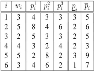
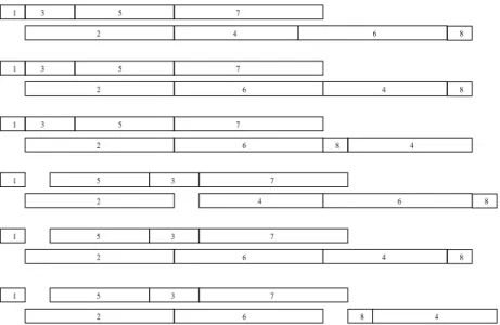
As an illustration, consider a small size capital budgeting problem where profit uncer-tainty or imprecision is modelled with three discrete scenarios or with interval scenarios. Numerical values are given in Table 1 withb = 12 and n = 6.
i wi p1i p2i p3i pi pi 1 3 4 3 3 3 5 2 5 8 4 6 2 6 3 2 5 3 3 2 5 4 4 3 2 4 2 3 5 5 2 8 2 3 9 6 3 4 6 2 1 7
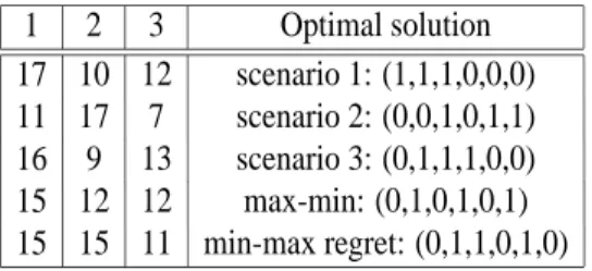
1 2 3 Optimal solution 17 10 12 scenario 1: (1,1,1,0,0,0) 11 17 7 scenario 2: (0,0,1,0,1,1) 16 9 13 scenario 3: (0,1,1,1,0,0) 15 12 12 max-min: (0,1,0,1,0,1) 15 15 11 min-max regret: (0,1,1,0,1,0)
Table 2: Optimal values and solutions (discrete scenario case)
In the discrete scenario case, we observe in Table 2 that the optimal solutions of the three scenarios are not completely satisfactory since they give low profits in some scenar-ios. An appropriate solution should behave well under any variation of the future profits. In this example, optimal solutions to max-min and min-max regret versions are more ac-ceptable solutions since their performances are more stable. A risk-averse decision maker would favor the max-min solution that guarantees at least 12 in all scenarios. If the deci-sion maker is willing to accept a small degradation of the performance in the worst case scenario with an increase of the average performance over all scenarios, then the optimal solution of the min-max regret version is more appropriate than the optimal solution of the min-max version.
In the interval scenario case, the optimal solution to the max-min version is obtained by considering only the worst-case scenario (see section 3.2) and corresponds tox1 =
x3= x5= 1; x2= x4= x6= 0 with a worst value 8. The obtained solution only depends on one scenario and, in particular, is completely independent of the interval upper bound values. An optimal solution of the min-max regret version is given byx1= x5= x6= 1;
x2= x3= x4= 0 with a worst value and a maximum regret 7. Unlike for the max-min criterion, the optimal min-max regret solution does depend on the interval lower and upper bound values. In particular, when an interval upper bound increases, the maximum regret of each feasible solution either increases or remains stable. Obviously, this may impact on the resulting optimal solution. For instance, if we increasep3 from 5 to 8, the new min-max regret optimal solution becomesx3= x5= x6= 1; x1= x2= x4= 0 with a worst value 6 and a maximum regret 8. Observe, in the previous example, that improving the prospects of investment 3 leads to include this investment in the new optimal solution.
2.3 Relevance and limits of the min-max (regret) criteria
When uncertainty or imprecision on the parameter values of decision aiding models is a crucial issue, decision makers may not feel confident using results derived from parame-ters taking precise values. Robustness analysis is a theoretical framework that enables the decision maker to take into account uncertainty or imprecision in order to produce
deci-sions that will behave reasonably under any likely input data (see, e.g., Roy [42], Vincke [45] for general contexts, Kouvelis and Yu [30] in combinatorial optimization, and Mul-vey, Verderbel, and Zenios [39] in mathematical programming). Different criteria can be used to select among robust decisions. The min-max and min-max regret criteria are often used to obtain conservative decisions to hedge against variations of the input data [41]. We briefly review situations where each criterion is appropriate.
The min-max criterion is suited for non-repetitive decisions (construction of a high voltage line, highway, . . . ) and for decision environments where precautionary measures are needed (nuclear accidents, public health). In such cases, classical approaches like deterministic or stochastic optimization are not relevant. This criterion is also appropriate in competitive situations [41] or when the decision maker must reach a pre-defined goal (sales, inventory, . . . ) under any variation of the input data.
The min-max regret criterion is suitable in situations where the decision maker may feel regret if he/she makes a wrong decision. He/she thus takes this anticipated regret into account when deciding. For instance, in finance, an investor may observe not only his own portfolio performance but also returns on other stocks or portfolios in which he was able to invest but decided not to [20]. Therefore, it seems very natural to assume that the investor may feel joy/disappointment if his own portfolio outperformed/underperformed some benchmark portfolio or portfolios. The min-max regret criterion reflects such a behavior and is less conservative than the min-max criterion since it considers missed opportunities. It has also been shown that, in the presence of uncertainty on prices and yields, the behavior of some economical agents (farmers) could sometimes be better pre-dicted using a min-max regret criterion, rather than a classical profit maximization crite-rion [29].
Maximum regret can also serve as an indicator of how much the performance of a decision can be improved if all uncertainties/imprecisions could be resolved [30]. The min-max regret criterion is relevant in situations where the decision maker is evaluated ex-post.
Another justification of the min-max regret criterion is as follows. In uncertain/impre-cise decision contexts, a reasonable objective is to find a solution with performances as close as possible from the optimal values under all scenarios. This amounts to setting a thresholdε and looking for a solution x ∈ X such that val(x, s) − val∗
s≤ ε, for all s ∈ S. Equivalently,x should satisfy Rmax(x) ≤ ε. Then, looking for such a solution with ε as small as possible is equivalent to determining a min-max regret solution.
Min-max and min-max regret criteria are simple to use since they do not require any additional information unlike other approaches based on probability or fuzzy set theory. Furthermore, they are often considered as reference criteria and a starting point in robust-ness analysis. However, the min-max and min-max regret criteria are sometimes inappro-priate. In some situations, these criteria are too pessimistic for decision makers who are
willing to accept some degree of risk. In addition, they attach a great importance to worst case scenarios which are sometimes unlikely to occur. In the discrete scenario case, this difficulty could be handled, at the modelling stage, by including only relevant scenarios in the scenario set. In the interval scenario case, min-max and min-max regret optimal solutions are obtained for extreme scenarios, as will be shown in section 3.2. Clearly not all these scenarios are likely to happen and this limits the applicability of these criteria. This difficulty becomes all the more important than the intervals get larger.
Some approaches have been designed so as to reduce these drawbacks. In the discrete scenario case, Daskin, Hesse, and ReVelle [19] propose a model called theα-reliable
min-max regret model that identifies a solution that minimizes the maximum regret with respect to a selected subset of scenarios whose probability of occurrence is at least some user-defined valueα. Kalai, Aloulou, Vallin, and Vanderpooten [25] propose another
approach called lexicographicα-robustness which, instead of focusing on the worst case,
considers all scenarios in lexicographic order, from the worst to the best, and also includes a tolerance thresholdα in order not to discriminate among solutions with similar values.
In the interval scenario case, Bertsimas and Sim [15] propose a robustness model with a scenario set restricted to scenarios where the number of parameters that are pushed to their upper bounds is limited by a user-specified parameter. The robust version obtained using this model has the same approximation complexity as the classical version. This is a clear advantage over the classical robustness criteria since their robust counterpart are generally NP-hard. The main difficulty is, however, the definition of this technical parameter whose value may impact on the resulting solution.
3 General results on min-max (regret) versions
We present in this section general results that give an insight on the nature and dif-ficulty of min-max (regret) versions. They also serve as a basis for further results or algorithms presented in the next sections.
3.1 Discrete scenario case
3.1.1 Relationships between min-max (regret) and classical versions
We investigate, in this part, the quality of the solutions obtained by solvingP for
specific scenarios.
A first attempt to solve DISCRETEMIN-MAX(REGRET)P is to construct an optimal
solutionx∗
sfor each scenarios ∈ S, compute maxs∈Sval(x∗s, s) (or Rmax(x∗s)), and then, select the best of the obtained candidate solutions. However, this solution can be very
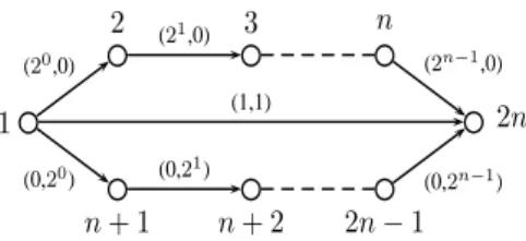
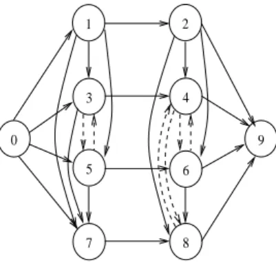
bad, since the gap between its value and the optimal value may increase exponentially in the size of the instance as we can see in the following example. Consider for example a pathological instance of DISCRETEMIN-MAX(REGRET) SHORTESTPATH. Figure 1 depicts a graphG = (V, A) with 2n vertices where each arc is valued by costs on 2
scenarios. The optimal solution in the first scenario is given by path1, n+1, . . . , 2n−1, 2n
with values(0, 2n− 1), a worst value 2n − 1 and a maximum regret 2n− 1, whereas the optimal solution in the second scenario is given by path1, 2, . . . , n, 2n with values (2n− 1, 0), a worst value 2n− 1, and a maximum regret 2n− 1. However, the optimal solution of the min-max and min-max regret versions is given by path1, 2n with a worst
value 1 and a maximum regret 1. Thus the gap between the best value (regret) among the optimal solutions of each scenario and the optimum of min-max (min-max regret) is
2n− 2. 1 2 3 n n+ 1 n+ 2 2n − 1 2n (20,0) (0,20) (2n−1,0) (0,2n−1) (21,0) (0,21) (1,1)
Figure 1:A critical instance of DISCRETEMIN-MAX(REGRET) SHORTESTPATHwhere opti-mal solutions in each scenario are very bad
The previous example shows that by solvingP for all scenarios in S, we cannot
guar-antee the performance of the obtained solution. Another idea is to solve problemP for
a fictitious scenario in the hope that the obtained solution has a good performance. The following proposition considers the median scenario, i.e. with costs corresponding to the average value over all scenarios.
Proposition 1 ([30]) Consider an instanceI of DISCRETEMIN-MAXP (or DISCRETE
MIN-MAX REGRET P) with k scenarios where each scenario s ∈ S is represented
by (cs
1, . . . , csn) and where P is a minimization problem. Consider also an instance
I′ of P where each coefficient of the objective function is defined by c′ i = Pk s=1 cs i k,
i = 1, . . . , n. Then x′an optimal solution ofI′is such thatmax
s∈Sval(x′, s) ≤ k.opt(I)
(orRmax(x′) ≤ k.opt(I)) where opt(I) denotes the optimal value of instance I.
Proof : Consider an instance I of DISCRETE MIN-MAX REGRET P. Let x′ be an optimal solution ofI′. We first show thatL =P
s∈S1k(val(x′, s) − val∗s) is a lower bound ofopt(I). L = min x∈X 1 k X s∈S
(val(x, s) − val∗s) ≤ min
x∈X
1
kk maxs∈S(val(x, s) − val ∗
Moreover,U = maxs∈S(val(x′, s) − val∗s) is clearly an upper bound of opt(I) and we get
min
x∈Xmaxs∈S(val(x, s) − val ∗
s) ≤ maxs∈S(val(x′, s) − val∗s) ≤
X
s∈S
(val(x′, s) − vals∗)
= kL ≤ k.opt(I)
The proof for DISCRETE MIN-MAX P is exactly the same except that we take L = P
s∈S1kval(x′, s) and U = maxs∈Sval(x′, s) as lower and upper bounds of opt(I), and we removeval∗
severywhere in the proof. 2
Considering a maximization problemP, we can define lower and upper bounds L and U similarly. For the min-max regret version, we also obtain a k-approximate solution
in this way. However, the previous result does not hold for the max-min version since the ratio UL is not bounded. In particular, for the knapsack problem, this ratio can be exponential in the size of the input, as noticed in [49].
An alternative idea is to solve problemP on a fictitious scenario, called pessimistic
scenario, with costs corresponding to the worst values over all scenarios.
Proposition 2 Consider an instanceI of DISCRETEMIN-MAXP with k scenarios where each scenarios ∈ S is represented by (cs
1, . . . , csn) and where P is a minimization
prob-lem. Consider also an instanceI′ofP where each coefficient of the objective function is
defined byc′
i = maxs∈Scsi,i = 1, . . . , n. Then x′an optimal solution ofI′is such that
maxs∈Sval(x′, s) ≤ k.opt(I) where opt(I) denotes the optimal value of instance I.
Proof : Letx∗denote an optimal solution of instanceI. We have
max s∈S n X i=1 csix′i≤ n X i=1 c′ix′i≤ n X i=1 c′ix∗i ≤ n X i=1 X s∈S csix∗i =X s∈S n X i=1 csix∗i ≤ k. max s∈S n X i=1 csix∗i = k.opt(I) 2
The same result cannot be extended to the min-max regret version. Figure 2 illustrates a critical instance of DISCRETEMIN-MAXREGRETSHORTESTPATHwith two scenar-ios. The optimal solution for the first and second scenario is the same and corresponds to path1, n − 1, n. Thus, this path is the min-max regret optimal solution with a
maxi-mum regret 0. However, the optimal solution for the pessimistic scenario is given by path
1 2 3 4 n − 2 n− 1 n (2n, 2n) (0,2n + 1) (2n, 2n) (0, 0) (0, 0) (2n ,0)
Figure 2: A critical instance of DISCRETE MIN-MAXREGRET SHORTEST PATHwhere the optimal solution in the pessimistic scenario is very bad
Extension of Proposition 2 to a maximization problemP does not hold neither for
DISCRETEMAX-MINP nor for DISCRETEMIN-MAXREGRETP.
Quite interestingly, however, solvingP for the pessimistic scenario leads to optimal
solutions for the specific class of bottleneck problems defined as
½
min maxi=1,...,ncixi ci∈ N
x ∈ X ⊂ {0, 1}n
This class encompasses bottleneck versions of classical optimization problems (short-est path, spanning tree, . . . ). The min-max and min-max regret bottleneck versions are defined by (1) and (2) respectively, withval(x, s) = maxi=1,...,ncsixi.
These versions are denoted DISCRETE MIN-MAX (REGRET) BOTTLENECKP in
the discrete scenario case, and INTERVALMIN-MAX(REGRET) BOTTLENECKP in the
interval scenario case.
Proposition 3 Consider an instanceI of DISCRETEMIN-MAX BOTTLENECKP with k scenarios where each scenario s ∈ S is represented by (cs
1, . . . , csn) and where P is a
minimization problem. Consider also an instanceI′ofP where each coefficient of the
objective function is defined byc′
i= maxs∈Scsi,i = 1, . . . , n. Then x′an optimal solution
ofI′is also an optimal solution ofI.
Proof :
min
x∈Xmaxs∈S val(x, s) = minx∈Xmaxs∈S i=1,...,nmax c s
ixi= min
x∈Xi=1,...,nmax maxs∈S c s ixi= min x∈Xi=1,...,nmax c ′ ixi 2
The next proposition gives a reduction from DISCRETE MIN-MAX REGRET BOT
Proposition 4 Consider an instanceI of DISCRETEMIN-MAXREGRETBOTTLENECK P with k scenarios where each scenario s ∈ S is represented by (cs
1, . . . , csn) and where
P is a minimization problem. Consider also an instance eI of DISCRETE MIN-MAX
BOTTLENECK P where each coefficient of the objective function is defined by ecsi = max{cs
i − val∗s, 0}, i = 1, . . . , n. Then ex, an optimal solution of eI, is also an optimal
solution ofI.
Proof :
min
x∈Xmaxs∈S(val(x, s) − val ∗
s) = minx∈Xmaxs∈S( maxi=1,...,ncsixi− vals∗) = minx∈Xmaxs∈S i=1,...,nmax ecsixi
2
The previous propositions are summarized in the following corollary.
Corollary 1 GivenP an optimization problem, DISCRETEMIN-MAXBOTTLENECKP and DISCRETEMIN-MAXREGRETBOTTLENECKP reduce to P.
3.1.2 Relationships between min-max (regret) and multi-objective versions
It is natural to consider scenarios as objective functions. This leads us to investigate relationships between min-max (regret) and multi-objective versions.
The multi-objective version associated to P ∈ C, denoted by MULTI-OBJECTIVE P, has for input k objective functions where the hth objective function has coefficients ch
1, . . . , chn. We denote byval(x, h) =
Pn
i=1chixithe value of solutionx ∈ X on criterion
h, and assume w.l.o.g. that all criteria are to be minimized. Given two feasible solutions x and y, we say that x dominates y if val(x, h) ≤ val(y, h) for h = 1, . . . , k with at least
one strict inequality. The problem consists of finding the setE of efficient solutions. A
feasible solutionx is efficient if there is no other feasible solution y that dominates x. In
general MULTI-OBJECTIVEP is intractable in the sense that it admits instances for which
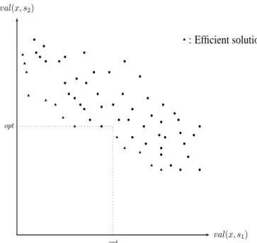
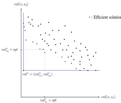
val(x, s2) val(x, s1) u u u u u u u u u u u u u b b b b b b b b b b b b b b b b b b b b b b b b b b b b b b b b b b b b b b b b b b b b b b b b b opt opt : Efficient solutions u
Figure 3: Relationships between min-max and multi-objective versions
Proposition 5 Given a minimization problemP, at least one optimal solution for DIS
-CRETEMIN-MAXP is necessarily an efficient solution.
Proof : Ifx ∈ X dominates y ∈ X then maxs∈Sval(x, s) ≤ maxs∈Sval(y, s). There-fore, we obtain an optimal solution for DISCRETEMIN-MAXP by taking, among the
efficient solutions, one that has a minimummaxs∈Sval(x, s), see Figure 3. 2
Proposition 6 Given a minimization problemP, at least one optimal solution for DIS
-CRETEMIN-MAXREGRETP is necessarily an efficient solution.
Proof : Ifx ∈ X dominates y ∈ X then val(x, s) ≤ val(y, s), for each s ∈ S, and thus Rmax(x) ≤ Rmax(y). Therefore, we obtain an optimal solution for DISCRETEMIN-MAX REGRET P by taking, among the efficient solutions, a solution x that has a minimum
val(x, s2) val(x, s1) u u u u u u u u u u u u u b b b b b b b b b b b b b b b b b b b b b b b b b b b b b b b b b b b b b b b b b b b b b b b b b b b val∗= (val∗ s1, val∗s2) val∗ s2+ opt val∗ s1+ opt : Efficient solutions u
Figure 4: Relationships between min-max regret and multi-objective versions Observe that if DISCRETEMIN-MAX(REGRET)P admit several optimal solutions,
some of them may not be efficient, but at least one is efficient (see Figures 3 and 4).
3.2 Interval scenario case
For a minimization problemP ∈ C, solving INTERVALMIN-MAXP is equivalent to
solvingP on the scenario c = (c1, . . . , cn) where the values of all coefficients ciare set to their upper bounds (for a maximization problem, consider only scenarioc = (c1, . . . , cn)).
Therefore, the rest of the section is devoted to INTERVALMIN-MAXREGRETP.
In order to compute the maximum regret of a solutionx ∈ X, we only need to consider
its worst scenarioc−(x). Yaman, Kara¸san and Pinar [48] propose an approach to construct this scenario for INTERVALMIN-MAX REGRETSPANNINGTREEand characterize the optimal solution. These approaches can, however, be generalized to any problemP ∈ C.
Proposition 7 Given a minimization problemP, the regret of a solution x ∈ X is maxi-mized for scenarioc−(x) defined as follows:
c−i(x) = ½
ci if xi= 1,
ci if xi= 0,
Proof : Given a solutionx ∈ X, let I(x) = {i ∈ 1, . . . , n : xi = 1}. For any scenario s ∈ S, we have R(x, s) = val(x, s) − val(x∗s, s) = X i∈I(x)\I(x∗s) csi− X i∈I(x∗s)\I(x) csi ≤ X i∈I(x)\I(x∗s) ci− X i∈I(x∗s)\I(x) ci = val(x, c−(x)) − val(x∗s, c−(x)) ≤ val(x, c−(x)) − val(x∗c−(x), c−(x)) = R(x, c−(x)) 2
The following proposition shows that an optimal solution of INTERVAL MIN-MAX
REGRETP is an optimal solution of P for one of the extreme scenarios.
Proposition 8 Given a minimization problemP, an optimal solution x∗ of INTERVAL MIN-MAXREGRETP corresponds to an optimal solution of P for at least one extreme scenario, in particular its most favorable scenarioc+(x∗) defined as follows:
c+i (x∗) = ½ ci if x∗ i = 1, ci if x∗i = 0, i = 1, . . . , n
Proof : Letx∗ denote an optimal solution of INTERVAL MIN-MAX REGRET P and
I(x) = {i ∈ 1, . . . , n : xi= 1}. For any s ∈ S, we have
val(x∗, s) − val(x∗ c+(x∗), s) = X i∈I(x∗)\I(x∗ c+(x∗)) cs i − X i∈I(x∗ c+(x∗))\I(x∗) cs i ≥ X i∈I(x∗)\I(x∗ c+(x∗)) ci− X i∈I(x∗ c+(x∗))\I(x∗) ci = val(x∗, c+(x∗)) − val(x∗c+(x∗), c +(x∗)) Suppose thatx∗ is not an optimal solution ofP for its most favorable scenario c+(x∗). Then the previous expression is strictly positive. Consequently, we have
val(x∗, s) − val∗s> val(x∗c+(x∗), s) − val
∗ s, for all s ∈ S thus max s∈S{val(x ∗, s) − val∗
s} > maxs∈S{val(x∗c+(x∗), s) − val
∗ s} This contradicts the optimality ofx∗for INTERVALMIN-MAXREGRETP.
The two previous propositions suggest the following direct procedure to solve exactly the min-max regret version. First construct an optimal solutionx∗
sfor each extreme sce-narios and compute Rmax(x∗s) using Proposition 7. Then, select among these solutions one having the minimum maximum regret. This procedure is in general impracticable since the number of extreme scenarios is up to2n. Nevertheless, if the numberu ≤ n of uncertain/imprecise coefficientsci, corresponding to non degenerate intervals, is constant or bounded by the logarithm of a polynomial function in the size of the input, then IN
-TERVAL MIN-MAXREGRETP has the same complexity as P, as noticed by Averbakh
and Lebedev [14].
As for the discrete scenario case, we briefly investigate the quality of the solutions obtained by solvingP on a specific scenario.
A first idea, is to consider the worst scenarioc = (c1, . . . , cn), that is to take an optimal min-max solution as a candidate solution for the min-max regret version.
An optimal solution of INTERVALMIN-MAXP has, in practice, a maximum regret
close to the optimal value of the min-max regret version but, in the worst case, its perfor-mance is very bad. Figure 5 presents a critical example for SHORTESTPATH. The optimal solution of the min-max version is given by path1, n with a worst value and a maximum
regret2n. On the other hand, the optimal solution of the min-max regret version is given by path1, 2, . . . , n with a worst value 2n+ 1 and a maximum regret 1.
1 2 3 4 n− 1 n [0, 2n + 1] 2n 0 0 0
Figure 5: A critical instance of INTERVALMIN-MAX REGRET SHORTEST PATHwhere the optimal min-max solution is very bad
Kasperski and Zieli´nski [28] show that, by solving problemP on a particular scenario,
we can obtain a good upper bound of the optimal value of INTERVALMIN-MAXREGRET P.
Proposition 9 ([28]) Given an instanceI of INTERVALMIN-MAXREGRETP, consider an instanceI′ ofP where each coefficient of the objective function is defined by c′
i = 1
2(ci + ci). Then x′ an optimal solution of I′ has Rmax(x′) ≤ 2opt(I) where opt(I)
denotes the optimal value of instanceI.
For the class of bottleneck problems, as for the discrete scenario case (see Propositions 3 and 4), an optimal solution of INTERVALMIN-MAXREGRETBOTTLENECKP can be
obtained by solving BOTTLENECKP on a carefully selected scenario. Let si denote the scenario whereci= ciandcj= cjforj 6= i, and i = 1, . . . , n.
Proposition 10 ([9]) Given an instanceI of INTERVALMIN-MAX REGRETBOTTLE
-NECKP, consider an instance I′of BOTTLENECKP where each coefficient of the objec-tive function is defined byc′
i = max{ci− vals∗i, 0}. Then x
′an optimal solution ofI′is
also an optimal solution ofI.
4 Complexity of min-max and min-max regret versions
Complexity of the min-max (regret) versions has been studied extensively during the last decade. Clearly, the min-max version of problemP is at least as hard as P since P is a particular case of DISCRETE MIN-MAXP when the scenario set contains only
one scenario andP is a particular case of INTERVALMIN-MAXP when all coefficients
are degenerate. Similarly, the min-max regret version ofP is at least as difficult as P
sinceP reduces to DISCRETE(INTERVAL) MIN-MAXREGRETP when the scenario set
is reduced to one scenario. For this reason, in the following, we consider only min-max (regret) versions of polynomial or pseudo-polynomial time solvable problems, for which we could hope to preserve the complexity.
For the discrete scenario case, Kouvelis and Yu [30] give complexity results for sev-eral combinatorial optimization problems, including SHORTESTPATH, SPANNINGTREE, ASSIGNMENT, and KNAPSACK. In general, these versions are shown to be harder than
the classical versions. More precisely, if the number of scenarios is non-constant (the number of scenarios is part of the input), these problems become strongly NP-hard, even when the classical problems are solvable in polynomial time. On the other hand, for a constant number of scenarios, it is only partially known if these problems are strongly or weakly NP-hard. Indeed, the reductions described in [30] to prove the NP-hardness are based on transformations from the partition problem which is known to be weakly NP-hard [23]. These reductions give no indications on the precise status of these problems. Most of the problems which are known to be weakly NP-hard are those for which there exists a pseudo-polynomial algorithm based on dynamic programming [30] (MIN-MAX
(REGRET) SHORTESTPATH, MAX-MINKNAPSACK, MIN-MAXREGRETKNAPSACK,
MIN-MAX(REGRET) SPANNINGTREEon grid graphs, . . . )
As an example for this family of algorithms, we describe a pseudo-polynomial algo-rithm to solve DISCRETEMAX-MINKNAPSACK. The standard procedure to solve the classical knapsack problem is based on dynamic programming. We give an extension to the multi-scenario case which is very similar to the procedure presented in [22] by Er-lebach, Kellerer and Pferschy to solve multi-objective knapsack problem. This procedure is easier and more efficient than the one originally presented by Yu [49].
Consider a knapsack instance where each itemi has a weight wi and profitpsi, for
LetWi(v1, . . . , vk) denote the minimum weight of any subset of items among the first
i items with profit vsin each scenarios ∈ S. The initial condition of the algorithm is given by settingW0(0, . . . , 0) = 0 and W0(v1, . . . , vk) = b + 1 for all other combinations. The recursive relation is given by:
Ifvs≥ psi for alls ∈ S, then
Wi(v1, . . . , vk) = min{Wi−1(v1, . . . , vk), Wi−1(v1− p1i, . . . , vk− pki) + wi} else Wi(v1, . . . , vk) = Wi−1(v1, . . . , vk)
fori = 1, . . . , n.
Each entry ofWnsatisfyingWn(v1, . . . , vk) ≤ b corresponds to a feasible solution with profitvsin scenarios. The set of items leading to a feasible solution can be deter-mined easily using standard bookkeeping techniques. The feasible solutions are collected and an optimal solution to DISCRETE MAX-MIN KNAPSACK is obtained by picking a feasible solution minimizingmaxs∈Svs. Since,vs ∈ {0, . . . ,Pni=1psi}, the running time of this approach is given by going through the complete profit space for every item that isO(n(maxs∈SPni=1psi)k). The algorithm presented by Yu [49] has a running time
O(nb(maxs∈SPni=1psi)k).
SPANNINGTREEis not known to have a dynamic programming scheme but can be
solved, for instance, using Kruskal’s algorithm or Prim’s algorithm. A specific pseudo-polynomial algorithm is given in [3] for DISCRETEMIN-MAXSPANNINGTREEusing an extension of the matrix tree theorem to the multi-scenario case.
Aissi, Bazgan, and Vanderpooten investigate in [2] the complexity of min-max and min-max regret versions of two closely related polynomial-time solvable problems: CUT
ands−t CUT. For a constant number of scenarios, the complexity status of these problems
is widely contrasted. More precisely, DISCRETEMIN-MAX(REGRET) CUTare polyno-mial, whereas DISCRETE MIN-MAX(REGRET)s − t CUTare strongly NP-hard even
for two scenarios. It is interesting to observe thats − t CUTis the first polynomial-time solvable problem, whose min-max and min-max regret versions are strongly NP-hard.
Network location models are characterized by two types of parameters (weights of nodes and lengths of edges) and by a location site (on nodes or on edges). Kouvelis and Yu [30] show that DISCRETE MIN-MAX (REGRET) 1-MEDIANcan be solved in polynomial time for trees with scenarios both on node weights and edge lengths. If the location sites are limited to nodes, DISCRETEMIN-MAX(REGRET) 1-MEDIANcan be solved in polynomial time using an exhaustive search algorithm.
The complexity of the min-max (regret) versions of scheduling problems has also been investigated. Daniels and Kouvelis [18] show that DISCRETEMIN-MAX(REGRET)
1|prec|fmaxis polynomial-time solvable whereas DISCRETEMIN-MAX1||PUjis NP-hard.
In the interval scenario case, extensive research has been devoted for studying the complexity of min-max regret versions of various optimization problems including SHORT
-ESTPATH[14], SPANNINGTREE[8, 14], ASSIGNMENT[1], CUTands − t CUT[2]. In general, all these problems are shown to be strongly NP-hard.
For network locations problems, if edge lengths are uncertain/imprecise, INTERVAL
MIN-MAX REGRET 1-MEDIAN is shown to be strongly NP-hard for general graphs
[11] but polynomial-time solvable on trees [17]. However, if vertex weights are uncer-tain/imprecise, this problem is polynomial-time solvable [13]. For 1-CENTER, a closely
related problem, INTERVALMIN-MAXREGRET1-CENTERis shown to be strongly NP-hard for general graphs if edge lengths are uncertain/imprecise but polynomial-time solv-able on trees [13]. Nevertheless, if vertex weights are uncertain/imprecise, this problem is polynomial-time solvable [12].
For scheduling problems, Kasperski [27] shows that INTERVALMIN-MAXREGRET 1|prec|fmaxis polynomial-time solvable. Lebedev and Averbakh [31] show that INTER
-VALMIN-MAXREGRET1||PwjCjis NP-hard.
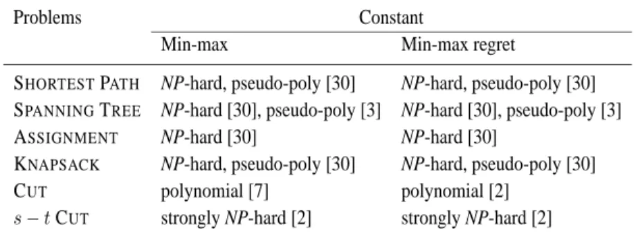
Tables 3-5 summarize the complexity of min-max (regret) versions of several classical combinatorial optimization problems. For all studied problems, min-max and min-max regret versions have the same complexity in the discrete scenario case. In general, there is no reduction between the min-max and the min-max regret versions or vice versa. However, in all known reductions establishing the NP-hardness of min-max versions [30, 1, 2], the obtained instances of min-max versions have been designed so as to get an optimal value on each scenario equal to zero. This way, these reductions also imply the
NP-hardness of the min-max regret associated versions. Comparing now the complexity
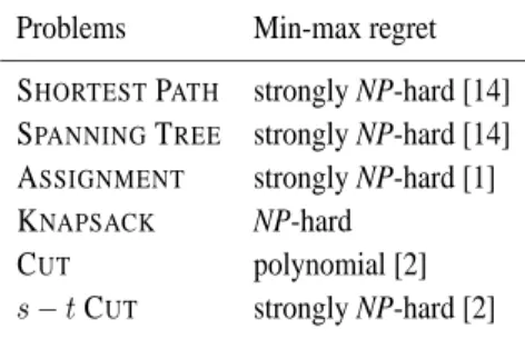
of the min-max regret version in the discrete scenario case and in the interval scenario case, we observe some slight differences. As shown by Averbakh [10], there even exists a simple combinatorial optimization problem, the selection problem, whose min-max regret version is solvable in polynomial time in the interval scenario case whereas it is NP-hard even for two scenarios.
Table 3: Complexity of the min-max (regret) versions of classical combinatorial problems (constant number of scenarios)
Problems Constant
Min-max Min-max regret
SHORTESTPATH NP-hard, pseudo-poly [30] NP-hard, pseudo-poly [30]
SPANNINGTREE NP-hard [30], pseudo-poly [3] NP-hard [30], pseudo-poly [3]
ASSIGNMENT NP-hard [30] NP-hard [30]
KNAPSACK NP-hard, pseudo-poly [30] NP-hard, pseudo-poly [30]
CUT polynomial [7] polynomial [2]
s− t CUT strongly NP-hard [2] strongly NP-hard [2]
Table 4: Complexity of the min-max (regret) versions of classical combinatorial problems (non-constant number of scenarios)
Problems Non-constant
Min-max Min-max regret SHORTESTPATH strongly NP-hard [30] strongly NP-hard [30] SPANNINGTREE strongly NP-hard [30] strongly NP-hard [4] ASSIGNMENT strongly NP-hard [1] strongly NP-hard [1] KNAPSACK strongly NP-hard [30] strongly NP-hard [4] CUT strongly NP-hard [2] strongly NP-hard [2]
s− t CUT strongly NP-hard [2] strongly NP-hard [2]
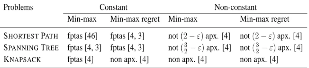
5 Approximation of the min-max (regret) versions
The approximation of the min-max (regret) versions of classical combinatorial opti-mization problems has received great attention recently. Aissi, Bazgan, and Vanderpooten initiated in [4] a systematic study of this question in the discrete scenario case. More precisely, they investigate the relationships between min-max, min-max regret and multi-objective versions, and show the existence, in the case of a constant number of scenarios, of fully polynomial-time approximation schemes (fptas) for min-max (regret) versions of several classical optimization problems. They also study the case of a non-constant number of scenarios. In this setting, they provide non-approximability results for min-max (regret) versions of shortest path and spanning tree. In [3] they adopt an alternative
Table 5: Complexity of min-max regret versions of classical combinatorial problems (in-terval scenario case)
Problems Min-max regret SHORTESTPATH strongly NP-hard [14] SPANNINGTREE strongly NP-hard [14] ASSIGNMENT strongly NP-hard [1] KNAPSACK NP-hard
CUT polynomial [2]
s− t CUT strongly NP-hard [2]
perspective and develop a general approximation scheme, using the scaling technique, which can be applied to min-max (regret) versions of some problems, provided that some conditions are satisfied. The advantage of this second approach is that the resulting fptas usually have much better running times than those derived using multi-objective fptas for the multi-objective versions.
The interval scenario case has been much less studied. We only report one general result due to Kasperski and Zieli´nski [28].
5.1 Discrete scenario case
As a first general result, Proposition 1 gives ak-approximation algorithm for DIS
-CRETE MIN-MAX (REGRET) P when the underlying problem P is polynomial-time
solvable. In some cases, however, we can derive fptas for some problems.
5.1.1 Relationships between min-max (regret) and multi-objective versions
Exploiting the results mentioned in section 3.1.2 concerning the relationships with the multi-objective version, we can derive approximation algorithms, with a noticeable difference between the min-max and the min-max regret versions.
Min-max version
Proposition 11 ([4]) Given a minimization problemP, for any function f : IN → (1, ∞), if MULTI-OBJECTIVEP has a polynomial-time f(n)-approximation algorithm, then DIS