Can diversification degree amplify momentum and contrarian anomalies ?

Co-authored by:

Houda BEN MHENNI HAJ YOUSSEF Economics and Applied Finance Research Unit The Institute of High Commercial Studies Carthage, Tunisia

hbenmhenni@ yahoo.fr (216) 21 32 76 48 Lassad EL MOUBARKI Paris Dauphine University elmoubarki_lassad@yahoo.fr

(216) 97 37 91 04

Olfa BENOUDA SIOUD Associate Professsor

Economics and Applied Finance Research Unit The Institute of High Commercial Studies Carthage, Tunisia

olfa.benouda@ihec.rnu.tn (216) 98 64 80 64

Abstract

This paper analyses the impact of industrial diversification on the profitability of contrarian and momentum strategies. Our findings show that the momentum strategy seems to be no more profitable in the recent years. In fact, while momentum strategies earn large positive and significant returns before the 2000 crash, these returns are negative after the crash. Then, firms are classified into two groups according to the intensity of their industrial diversification by the Ward (1963) method. We find that, for the non -diversified sample, no effect is significant. However, for the diversified sample, the significant contrarian effect observed in the medium term disappears in the long run. Before the crash, we find a more pronounced momentum effect for the non -diversified sample. After the

crash, we identify a contrarian effect more important for this sample. Moreover, the Bootstrap without replacement results do not support the risk based explanation.

Keywords : corporate diversification, mo ment u m, Bootstrap, cross-sectional variance of expected return, risk

1.

I

The momentum and contrarian anomalies have been witnessed not only in the American market but also in many international financial markets (Patro and Wu, 2004; Lewellen, 2002; Rouwenhorst, 1998; Richards, 1997). Based on the fact that the best (bad) performing stocks will continue their upward (downward) trend, the momentum strategies, which consist in buying stocks with high returns (winners) and selling stocks with low return (losers), are profitable in the medium run (Jegadeesh and Titman 1993). In the long run, the trend will reverse and the contrarian strategy, implying a long position in the past losers and short position in the winners, will be profitable during 3-5 years (DeBondt and Thaler, 1985, 1987).

Two competing approaches are put forward to account for the profitability of these trading strategies: the first is the rational approach that consists in explaining the momentum anomaly by systematic factors of the risk ignored by the standard models. The second is the behavioral approach that explains the strategy’s profits by judgment biases. These judgment biases induce investors’ over-reaction or under-reaction to information and produce continuation and of stock returns’ reversals. The behavioral models also suggest that momentum and contrarian effects should be more severe for firms that are hard-to-value (Daniel and Titman 1999) and suffering from a higher level of informational asymmetry (Jegadeesh and Titman 2001).

Prior studies recorded a significant relation between industrial diversification and information asymmetry.Nonetheless, they offer contradictory predictions about how diversification affects the level of information asymmetry. On the one hand, the degree of information asymmetry between managers and outsiders may differ for the diversified versus the focused firms. The reason is twofold. First, diversified firms are required to report only limited accounting information for their business segment. Therefore, diversified firms’ managers can observe divisional cash- flows while outsiders can observe only noisy estimates of divisional cash flows (Rajan et al. 2000; Nanda and Narayanan, 1999). Aware of this advantage, managers may manage earnings and exercise considerable discretion in allocating revenues, costs, and assets across the business segments (Givoly et al. 1999; Dunn and Nathan, 1998). Thus, the consolidated nature of earnings for the diversified firms could actually imply less transparency to outsiders and reported earnings will convey less value-relevant information (Habib et al. 1997).

Second, diversified firms operate in many industries and have more complex structures while individual financial analysts often specialize within a particular industry (Boudoukh et al. 1994).Hence, analyzing the firm’s earnings reports requires more resources and expertise and dealing with a diversified firm will be a difficult task (Zuckerman, 2000; Dunn and Nathan, 1998). As a result, the degree of informational asymmetry is likely to be more acute in diversified firms.

On the other hand, corporate diversification may reduce the asymmetric information problems because of the aggregate nature of firms’ accounting reports. Indeed, firms that operate in different industries are likely to derive cash flows that are not perfectly correlated. Thus, the errors made by outsiders’ in predicting these cash flows are imperfectly or negatively correlated across the segments and the absolute value of the percentage error in the forecast of diversified firm’s consolidated cash flows may be lowered. In other words, if the errors that outsiders make in forecasting segment cash flows are not perfectly positively correlated then the consolidated forecast may be more precise for a diversified firm than a forecast for a focused firm. Therefore, the degree to which the predictions of outsiders differ from the managers’ private information could be reduced (Hadlock et al. 1999; Thomas, 2002; Clarke et al. 2004).

In brief, prior studies affirm that industrial diversification has an impact on the level of information asymmetry. The behavioral models also suggest that momentum anomaly is affected by information asymmetry. Specifically, they argue that the momentum (and contrarian) effect is attributed to inefficient stock price reaction to the firm’s specific information (Jegadeesh and Titman, 2001). Empirical evidence support that it is related to various proxies for the quality and type of information that is provided about the firm, the relative amounts of information disclosed publicly and being generated privately (Hong et Stein, 1999). Therefore, mispricing should be more severe among securities that are hard to value and momentum and contrarian effects are likely to be greater. Thus, this paper aims to study the impact of industrial diversification on the profitability of contrarian and momentum strategies. If industrial diversification decreases the level of asymmetric information, the momentum and contrarian effects must be less pronounced for the diversified firms. Contrarily, if industrial diversification increases the level of asymmetric information, the momentum and contrarian effects must be less pronounced for the diversified firms.

Using Monthly returns, the WRSS strategy were applied to 249 American listed stocks from January 1994 to April 2004. In contrast to previous studies using older data, our results show that the momentum strategy seems to stop being profitable. To study the impact of the 2000 crash on our results, we implement the WRSS strategy during the [01/1994-03/2000] and [04/2000-04/2004] sub-periods. Our results indicate that while momentum strategies earn

large positive and significant returns during the first sub- period, these returns are negative during the second sub- period. As Hong and Stein (2003) report, the 2000 market crash is qualified by negative returns.

Then, firms are classified according to the intensity of their industrial diversification by Ward‘s (1963) method of hierarchical cluster analysis. According to this method, our sample should be classified into two sub-samples: the diversified and non diversified samples. By re-implementing the WRSS strategy on these sub-samples, we find that, for the non diversified sample, no effect is significant. However, for the diversified sample, the significant contrarian effect observed in the medium term disappears in the long run. Before the crash, we find a momentum effect more pronounced for the non diversified sample. After the crash, we note a contrarian effect which is more important for this sample. The Bootstrap without replacement is used to explore the risk- based explanation of the profitability of trading strategies. Our results imply that the cross-sectional difference in expected returns does not, entirely, explain the trading strategies’ profits.

Our investigation extends the literature both in behavioural finance and corporate diversification. Really, it’s noteworthy to verify the persistence of the momentum and contrarian anomalies in recent years for two reasons: The first is to avoid data mining problems and the second is to assess the extent to which investors have learned from earlier trends. Moreover, many studies revealed that the contrarian or momentum portfolios formed by firm characteristics such as size, book-to-market, and/or dividend can yield a significant positive return. Nevertheless, in spite of its importance, industrial diversification remains not studied.

Also, our study contributes to the literature on corporate diversification. According to the latest surveys, the values of diversified firms are discounted compared with non diversified firms (Jensen, 1986; Stulz, 1990; Denis, et al., 1997). We provided evidence that diversified firms are more efficiently valued. In fact, before the crash, the non diversified firms were more overvalued and after the crash they become more undervalued.

The paper is outlined as follows. Section 1 presents a literature review. Section 2 introduces the sample and the methodology. As for the results, they are presented in section 3, while alternative explanations are examined in section 4, and we shall conclude our research in the last section.

2.

Literature review: Momentum and Contrarian effects

The profitability of contrarian and momentum strategies was confirmed by empirical studies1_{. Momentum}

portfolios, which entail long positions in the past best performing stocks (winners) and short positions in the past worst performing stocks (losers), yield significant positive profits in the medium term: 3–12 months (Jegadeesh and

1 _{Jegadeesh et Titman (1993), DeBondt et Thaler (1985), Daniel et al (1998), Barberis et al (1998), Hong et Stein}

Titman, 1993). In contrast, a systematic reversal effect is found when a longer holding period (more than 3 years) is considered, and reversing the momentum strategy (buying past losers and selling past winners) results in the production of contrarian profits (DeBondt and Thaler 1985).

While most of the empirical works point to some level of predictability in stock returns, the underlying

explanation for this type of predictability remains challenging. The rational approach asserts that the standard models like CAPM or the three -factor model fail to take into account the systematic risk (Fama, 1998). To bypass this shortfall, Conrad and Kaul (1998) adopt the bootstrap and Monte Carlo -simulation techniques. They find that momentum and contrarian profits are explained by the cross-sectional variance of the stocks’ expected returns: The momentum strategy tends to buy the stocks with higher than average unconditional mean returns and sell the stocks with lower than average mean returns, and hence the momentum effect is not related to stock predictability.

Advocates of the behavioral approach propose a number of theoretical models of investors’ behaviour to explain these serial correlation properties in stock prices. The underpinning of the Daniel et al. (1998) model is investor overconfidence. They consider that stock prices are determined by the informed investors who are subject to two biases: overconfidence and self-attribution. Overconfidence in their signals causes overreaction to their private information, and self-attribution causes under-reaction to public information. Overreaction to private information leads them to push up the prices of the winners above their fundamental values. This trend will be reversed, in the long run, when public information will be confirmed.

Baberis et al. (1998) present a pattern consisting of a representative investor who believes that earnings tend to move between two different “regimes”. In regime A, earnings are mean reverting and in regime B earning are trending. Specifically, when a positive earnings surprise is followed by another positive (negative) surprise, the investor raises the likelihood that he is in the trending regime, he tends to become too optimistic (pessimistic) about the future profitability of the firm. As a result, firms realizing good earnings’ growths tend to become overvalued, and those realizing bad earnings’ growths tend to become undervalued. The prices of these stocks ultimately undergo reversals as achieved earnings fail to meet expectations. Whereas when a positive surprise is followed by a negative surprise, the investor raises the likelihood that he is in the mean-reverting regime and he will under-react to earnings’ announcement. When this expectation is not confirmed by later earnings, stock prices show a delayed response to earlier earnings.

Hong and Stein (1999) propose a model which focuses on the interactions between heterogeneous agents rather than the psychology of the representative agent. The informed investors or the “news watchers” make forecasts based only upon private information. The other investors “momentum traders” condition only on the most

recent price change. The information obtained by the news watchers is broadcast slowly and hence is partially incorporated in the prices. This slow diffusion of information generates momentum. To benefit from the prices’ momentum, the momentum traders continue to trade pushing up the prices above their fundamental value and generating an overreaction that will be later reversed.

3. Sample and methodology

Momentum strategies will be profitable if stock returns display a positive serial correlation, whereas contrarian strategies will be profitable in case of negative serial correlation of stock returns. In order to examine the profits of these trading strategies, we employ the weighted relative strength strategy (WRSS) first proposed by Lo and MacKinlay (1990) and used by Conrad and Kaul (1998), Jegadeesh and Titman (2002), Lewellen (2002) to mention but a few. Under this strategy, investors hold assets in proportion to their market-adjusted returns. Specifically, they take long positions in stocks that have above average past returns and short stocks with below average past returns. So, the investment weight assigned to stock i at time t is given by

(

)

Where: N is the total number of stocks in the sample ri,t-1 is the return of stock i during ranking period t-1

Rt-1 is the average return across all stocks in the sample at time t-1

The profit of the WRSS strategy is given by:

it n it it

=

∑

W

r

π

ri,t is the return of stock i during holding period t

A positive (negative) profit indicates that a momentum (contrarian) strategy is profitable. As Conrad and Kaul (1998) highlight, this strategy has, at least, three advantages. First, it captures the philosophy of return-based trading strategies since its success depends on the time-series’ behavior of asset prices. Second, the weighing scheme reflects investor’s beliefs. Third, weights on all stocks sum up to zero; that is, they imply a zero-cost portfolio.

Our sample consists of 250 American firms listed from January 1, 1994, to April 30, 2004. Monthly returns are yielded from Datastream data files and the data for segment sales were taken from firm’s 10K annual reports published by the Securities and Exchange Commission (SEC).

We, first, implemented the WRSS strategy, on the entire sample, during different time periods ([1994, 2004]; [1994, 03/2000] and [04/2000, 04/2004]), for different holding periods (3, 6, 9 and 12 months) and for different ranking periods (3, 6, 9, 12 months). We stop our time period to March 2000 because it corresponds to the millennium crash and to be able to compare our results with prior studies. To minimize small-sample bias and raise the power of our tests, like Conrad and Kaul (1998) and Jegadeesh and Titman (2002), we construct trading strategies for overlapping holding periods on a monthly -frequency. Hence, we obtain 16 trading strategies for each time period. Then, firms of the sample are classified in two sub-samples according to their berry’s index: The diversified sample (Div) and the non diversified (NDiv) sample. We then re-implemented these strategies on these two sub-samples.

The Berry Index is an entropy measure of industrial diversification which takes into account both the number of segmentsin which a firm operates and the relative importance of each segment in total firm sales (Jacquemin and Berry, 1979; Palepu, 1985). This measure increases with the number of segments, holding constant variance of the segment size, and decreases with variance of the segment size, holding the number of segments constant. Thus, a two-segment firm with equal segment sales is more diversified than a two-segment firm with unequal segment sales. The lower bound of the Berry index is 0 (a single segment) and it tends to 1 for a highly diversified firm (but not equal to 1).

The Berry Index is defined as:

∑

Where n is the number of industrysegments in which the firm is active andPi is the share of the ith segment in the total sales of thefirm. Firms are taxonomised as diversified and non diversified by Hierarchical cluster -analysis. The Hierarchical cluster- analysis is a statistical method for finding relatively homogeneous clusters of cases based on measured characteristics. It starts with each case in a separate cluster and then combines the clusters sequentially, reducing the number of clusters at each step until only one cluster is left. When there are N cases, this involves N-1 clustering steps, or fusions. Ward (1963) put forward a clustering procedure that computes the distance between two

clusters. This popular method combines the two clusters at each stage which minimize the squared error function, or Euclidean sum of squares, E. Objective function E is defined as follows:

MinE = ΣkΣiεk (xi- µk)2

Where for a given classification, firm i belongs to cluster k, xi is the value of the Berry Index for the firm i, and µk is

the mean of Berry Index in cluster k. The summations are, firstly, the squared error of firm i in cluster k for the Berry Index; secondly, for all observations (firms) i within cluster k; and finally, to total the error over all clusters k. This hierarchical clustering process can be displayed as a tree, or dendrogram, where each step in the clustering process is illustrated by a join of the tree. The choice of the number of clusters in the classification tree relies on the Euclidean distances: A great distance between classes indicates a high degree of dissimilarity between classes. Each year we classify our sample firms according to their Berry Index ( the variable xi ). The ward methods’ tree,

displayed in figure 1, shows that our sample should be classified in two classes: Diversified and non diversified. In fact, the Euclidean distance is maximal for a number of classes equal two for all years.

1 70 2 3182_2110131287₁06₁5234₂₀927₂₁14₂₄₂82₁₂₂9₁₄14₂18391₁43₁₂₁₀7₂₄697₁₃0378841₁₂₁541₁₈352904800327594₁8951₁9₁₇₁₁₅55879₁₁3₁₅34265₁54₂₃35753₂₂7₁57₂0219₁₆09867₁₅68₁₁66₁₁₂321731₁₉02₁86₁61₁₆2₁₇412₁₂220399₁₇75₁4068₂5038₂28₂₂₃5₁₃7₁₅₆₂₃712251251492492482472456239234041222342302262242116222223222112082072050719012020421961951941939087111192191861851811781712176171771691675163159164948115101151471461421408121134913131241181514171611115398959392888783828180787776747372696866646260565554504947444039383533312928272625232214111098726631011091011 18036220133611994521023 8 16 496₂₄42189₁₀1 13 5 4 6 7 0 18 8 12 1 86 11 2 1 3632595043024₂₄313₁₁257101543₁₁₂₁9126120144213 0 10 20 30 40 hclust (*, "w ard") 1 70 2 31 22 99108₂12₁00₁2734₁₂32₁₃82₁066₁₀₂₀₂₀1₁₄9₂₄₂₁8₁₃8642₁₀₁₂₄75297₁5567₁₂2₁₃3₂₁494₁₅5₁7990425179₁₅3414846₁₈3581565183752₂8470₁52512148₁₈1298420322823723 5 8599₁₇3 13 7 1 7 1 58₁₅7535767₂₀2₁₉8819₁₆₂33₁60₂₂71619₁74₁63₁₀2₁₁3₁₅4₁6120₁₆52₁₆17₁₂122₂₄9₂₄8₂₄7₂₄5₂41₂4030₂346₂₂₃₂₃9₂26₂24₂₂3₂₂218₂₀₂₂₁1621₂₂₀7₂₀5₂04₂0195₁967₁₁₉0₂₀₁₉4₁₉3₁₉2₁₉15₁₈6₁₈87₁90₁₁81₁78₁₇7₁₇667₁69₁1₁₇2₁₇50₁51₁₁₅93₁₆5₁₆6₁₄748₁₄₁₁4943₁42₁₄0₁₃9₁₁₂4₁₂8₁₃4₁₃1₁₁8₁₁7₁16₁15₁₀5₁₀91₁₁4₁₁₁04₁039896959392888782818047787776737269686664626055940545569047444338353331292827262523_{221411109872621}7₁₁2868932₁₂₁11343₁₃6559₁₃3₂₃83645161345014421892183₁26₁206380₂0₂₁9₂₁₁₂561₁₉971315₂₁₁4420₁₁103024₂₄3 0 10 20 30 40 hclust (*, "w ard") 3 0 2 4 63 12 0 2 137 1 11 2 13 3 12 6 22 0 1 10 1 44961₁99₂1045₂₁9₂₄₁₆451₂48₂47₂₂403915₂₄₂₄622₂23₂4₂₂₂₂0₂₃34₂36₂₂₂1₂₁6₂05₂078₂₀1₂₁₂₁00971₂₀4₂₀₁₉6₁₉5₁₉4₁₉307₁₈91₁₉₁92₁₁₈₁₇1885₁86₁₁₇7₁₇6₁72₁7153_1616161697₁₅₁₄091₁₅9₁₅₁48₁47₁₄6₁₄33934₁₁₁40₁42₁₃1₁₂8₁24₁181₁₁5₁₁4₁₁₁₁67₁₁₁₀39896959392888782818078777674737269686665646260565554504947444340393835333129282726252322181514111098726₁₀05₁09₁4 ₁21586133251298599841225₅₉₁₄1732032282376130121101222023315811915420 2 16 0 1 98 2 27 10 2 16 853₁₅757₂₂₉₁₇9 23 517 1 37₂₄29097₁₃2₁₀63₁₂7₁₆₂₄6₁₀8₂₁167₂₃20₁₇8₁₃323483₁₆₂291₂0906₁₁41₁824₁₂7₂₁5₁₇730₁52₁₂₁8₁₁319₂06₂₁4375258414279₁₈3₁89₁53₁₅67594336244₁₅₅₁₇101238180616135489122451318448215701882146 0 1 0 2 0 3 0 4 0 5 0 hclust (*, "w ard") 2 49 2 484140₂₂₄₂₂₄75₂₃9₂₃6₂₃4₂₃0₂₂₂₂322426₂₂₂₁₂₁4316₂21₂₂₁1₂₀8₂07₂0496₁97₁0₂₀₂₀15₁₉4₁₉3₁₉2₁₉1₁₉₁₈56₁₈87₁90₁₁₇₁₇768₁₇1₁₈₁₇2₁₇1₁69₁67₁49₁509₁₆₁₅548₁47₁₄6₁₄3₁41₁₃40₁₃39₁₁17₁18₁4₁₂₁₂814₁₁11₁₁5₁₁65₁₀4₁₀398969593928887868281807877767473726968666564626056555450494443403938353332313029282726252322151411109826₁₀ 16451963371326591311321505212575154129115618425145180581892151318479188167041158711260823122091331259114410 6 61 19 9 11 0 18 3 12 1 24 3 15 1369701₁₇4₁₆024₁₂44367310711225₁₇281017016112167212901921882341092217100141166461005212283315216342062322137202227135172362415716821041553122113823374847229142119205314 5 22 51 1 29 17 9 13 0 17 3 2 37 2 4257 22 885991988489203 0 1 0 2 0 3 0 4 0 5 0 hclust (*, "w ard") 24 9 24 8 24 7 24 5 2 41 2 4040₂₃₂₃₂₃96₂₃₂₂6₂₂4₂₂₂₂23₂21₂161108₂₂₁₂4₂₁2096₁97₁₂₀₂₀104₂07₂4₁₉5₁₉₁₉₁₉2₁₉1₁90₁873₁₁817856_18181717216₁₇7₁₇₁69₁67₁₆5₁₅9₁₄7₁₄84950₁₁₁₁40393₁₄6₁₄₁₃4₁₃1₁₂8₁₂465₁₁18₁₁₁₁17₁₀4₁₀511₁14₁₁₀39895939288878682818078777674737269686665646260555450494443403935333231302928272625232214111098265₂₁3157₂₁4₁₆₁08₂₁33197₁₅5₂₃₁₅4₁₇3₂06₁791774853₁₂₁₃7166142920272022223227102168145225 1 12 9 19 8 20 38485₂₂8 13 0 2 375 7 24 299 12 25613₂209136₂₁₉₁₀9₁₃3714461₁385₁₂0₁₈₂₁₉9₁51₁369716₁₂₁₂₁₀6₁01₁10₂₄4₂₄345462470₁8952745921₁₈₁379₁₃5₁₂058₁5894₁₂35894251₂₀7075₁60₁₁55₁₅6₁₈441₂46938123₂₀816₁₈₁₇518₁53₂1537₁₆267₁₆14796890837₁₃₁₀₁52₁00₂₃163₁₁2019₂₁4413₁₁₆3₁₈2₁32₁134₂₁8 0 1 0 2 0 3 0 4 0 hclust (*, "w ard") 1 5 2 498₂₄7₂₄5₂₄1₂₄64₂₃40₂₃39₂₂₂₂3₂₂426₂30₂₂₂16141₂₂2₂₂₂₁1₂₀8₂07₂0476_1920192010₁95₁94₁87₁9021₁₉₁₉3₁₉876₁77₁₁₁₇1₁₈85₁86₁₇2₁₇19₁₆5₁₅79₁₆₁₆₁₁48479₁₄0₁₅₁₄6₁₄3₁₄0₁₃918₁₂34₁₃₁36₁₁₁₁₁7618₁24₁₁₁5₁₁4₁11₁05859₁₀9₁₀4393928887868281807737486777668726966564626055545049433935333234413029282726252322141098261135₂₄₁₆4₁₄5₂2512808₁₁₂₂3₂₀9₁₇3₁₉8284₁₃0₂₃799₁₃5068₂₂₄2₅₇₁₂2₂35_11023811627₁₆8₁₅953₁₃717₂76₂₃3₂₂9_17017232157_22720167182₁₂6₁42₂02633₁₂₂₃137_16147481000₁₈₄₀₁₄4₁₀1₁₅11₂₄4₁₂7790₁₂5₁₂6_2196119920₂313₅₆₂₁₁₃8₇₁₁₃391_1093645183383₉₄₁₂7564658₁79₂₄4163₁4₁8₁₅₁₅1048₂₁₂₁89_11334191889096₁55₁20_1182891107₁₅22₂₁2₂₀9₂₀5_174425116950₁84₁₀6₁₅3249721658₂₃₁₃5₁₇541_15621110 0 10 20 30 40 hclust (*, "w ard") 2 49 2 48 24 7 24 5 2 41 2 40 2 39 2 364₂₃0₂26₂24₂₃16₂₁3₂₂2₂₂₂₂87₂₀4₂₀1₂₁₂₁₂04₂01₂₀0₁₉79493₁₁₉₁65₁₉₁₉2₁₉10₁87₁86₁₉87₁₇₁₈₁₇15₁₈₁76₁72₁₇1₁₆9₁₅09₁₅65₁67₁₁₄9₁₄8₁47₁46₁₁363403_141412114828₁31₁₁17₁16₁₁5₁₁4_{103989593928887868281807877767473726968666564626055545049444339353332312927262523221411109826131}0415₁₁₁₀ 9₁₆4513214515712924192828292210782303248122859916619712122214624233161173771820220215381622171227315210221681271571302301750637122325367401845815415818246941602115496116172481135942120347230910015211634583415216151918931831231210831571417109902135175188562201102431336135123810139180457112611997991018961219281219715375152021153841232452163070244106144 0 10 20 30 40 hclust (*, "w ard") 2 49 2 48 24 7 24 5 2 41 2 40 23 9 23 6 23 4 23 0 2 26 2 242116₂₂₂₂₂₂32₂₁4₂₁1₂₀8₂₀7₂0104₂₂₀0₁₉7₁96₁95186₁870_191191993₁94₁2₁₈5₁₈17672₁₁₇₁7₁₇86765₁₁₇₁9₁₆1₁₄9₁₄8₁₄7₁₄61₁₃436₁₃₁40₁61₁₁₁₁₁₁281793893₁₀₁₀5928882818078777674737269686360558495450444393533312927262314119285₁3243_14347202341₁₀₁₆2₁₆3₂₁5106₁₇1₁₅59₁65741₁₁7₁₃₂₁₆27_1021864178₁₆6₂₃3385_21738209₂₁23536246₂₁₁₄5₂25₁33₁₄2₆₇₁₃0_23299227₁₂789₂₃884₁18₂₃5₁₀8_122371920753402₂₄8₁₂₂₂91₁00_1291315153_135349521587₁₀8₁₂₁₅1016₂₀89₁220₁₁9₁₇₄₆₁₇95_16197114₂₁3_2312217124₁₇29693_{181064045755215}3₉₄₁₅4_1562442871237_18184861143₅₁₁₁065_{1586270919021}802_{1602111792520}52₂₁9₆₁₁₉921₁₂6₅₆₁₅₁0_244304123220₁80859₂₄3₅₈₁₃9₁₈8₁₃8_1446671104₁25_10936115 0 1 0 2 0 3 0 4 0 hclust (*, "w ard") 1 5 2 498₂₄7₂45₂43₂₄96₂₃1₂₃0₂₄₂₄64₂₂34₂₂30₂₂₂23₂22₂₂1₂₁6₂0708₂14₂₁₂₁₂₀4₂₀1₂00₁97423_191919196₁₉5₁₈₁₈7690₁91₁₁₈5₁₈1₁₇9₁₇871₁72₁67₁₇₁₇₁₆9₁₆7₁65₁49₁₄06₁₄4748₁₁₁₃71₁₁34₁36₁₁₁6₁₁1₁05_{103989392888281807877767473726968636055545049443935333129272623141192813}047₁₈0₁₁201₁645₂₁385₁1943₁2₂₀₁₁₅7₃₄₂₁5393₁₆₂₃₁₅28_1622753122₁₇067₈₄₁₅336₁11716382₁₆₆₅₁₄13₂₃17₁73₂₁2₉₀₁₀4₂501₁₀₁₂₂45₁292937457₂0₁₃16620386971281181092374614252322824129812017466205282441601269192315861011256182541154305821936991310115135581413412217971220439111497641123713232101953161197542962018913209218102061551215172215212182183241538710312652594888184891877246621280454021701512415315894106 0 1 0 2 0 3 0 4 0 5 0 hclust (*, "w ard") 10 1 13 215₂₄9 2 48 2 4710₂₄₂₄₂₄53₂₄₂₃9₂₃6₂₃₂₃04₂26₂242116₂₂₂₂2₂₂3₂14₂118₂₀7₂04₂01₂₀7₂₀0₁₉₁₉6₁₉5₁₉4₁93₁92₁₁878601_19191717981₁₈5₁₈₁77₁76₁₇2₁₇19₁₄5₁₆67₁₁694640₁₁₄₁7₁₄8₁₃₁₃4₁₃1₁₁7653₁₀₁₁₀1116₁98939288828187807776747372696863655545042069443935333129271192847426231₂13₁645₁₆01039₁₂₁₁4₁₁92₁184₅₃₂₄0₁₈₁₃36₁₂2_1516584104385₁₄62₁093₁₁9₂15₁13_171202642338₂₁8₁₆22173₂₁₂₃73867₁₄1₂₂734₁₅7529₁29₅₂₁₄₁₅5₂9₂₂₁₃7128₁₀0₁₃037₂₂6637₁0₁₂3₂₀₁₀8₁₂0577₁₇₁₄2₄₆₂₃99685₁74₁₉8728₁₁5804₁₂₂₁694₇₀₁₀3₁₈₁₈2404512_15383107₂₀₁₂36139₁₉₁₀2₂₀9₁₂1₁75₂06₁₈9₁₅875₂₁210_2312295316397₁₆1163241_155611993646₁₁224₂₄68_{1815689425118}425₂₂056584₅₉₂₀4₂₄₈₇₁₁5₅₈₁₀930_13536125₁₂6_1441821154₁₅0₂₃828797191 0 1 0 2 0 3 0 4 0 5 0 hclust (*, "w ard") FIGURE 1 The Ward MethodTree

The centre and the number of stocks of each class are presented in Table 1. The number of stocks in the non -diversified sample is more important than the diversified sample until 1997. After this date, the number of diversified firms exceeded the number of non- diversified firms indicating that more firms have become diversified. The centres of the two classes have dropped from 1994 to 2003, while the non diversified sample, plummeted from 0.0535 in 1994 to 0.0077 in 2003.

TABLE 1

CENTRES AND NUMBER OF STOCKS

This implies that firms of the non -diversified samples became more and more specialized. Regarding the diversified sample, the centre has slightly fallen from 0.558 to 0.5238. These findings are similar to those of Wrigley (1970) According to this author, American firms chose to be highly- specialized or highly -diversified but not in the middle state.

We first implemented the strategies on the entire sample and for the [1994-1999] period because it matched with the time period used in the previous studies (Jegadeesh and Titman, 2001) and we will concentrate on the 6-month -ranking period strategies because they were the primary focus of the original Jegadeesh and Titman (1993)research.

4. Results

4.1

We first implemented the strategies on the entire sample and for the [01/1994-03/2000] period because it corresponds with the time period used in the early studies (Jegadeesh and Titman, 2001) and we will focus on the six month -ranking period strategies because they were the primary focus of the original Jegadeesh and Titman (1993) study.

Table 2 shows the profits of the trading strategies. For the [1994, 2004] time period, fourteen returns out of sixteen were negative, whereas only two returns were positive. Among the fourteen negative returns, four are not significant, four are significant at the 10% level and six are significant at the 5% level. The returns of six month- ranking period are all negative and are significant for the nine and twelve month- holding periods. The most

1994 1995 1996 1997 1998 1999 2000 2001 2002 2003

NDiv centers 0.0535 0.0458 0.02528 0.0028 0.0010 0.0008 0.0007 0.0013 0.0027 0.0077

number 159 159 148 126 121 119 116 98 102 107

Div centers 0.558 0.5534 0.5232 0.4908 0.4828 0.4894 0.4815 0.5068 0.5116 0.5238

profitable strategy is the 12-12 month contrarian strategy with a return of 1.3%. The return of the famous 6-6 month strategy is negative and not significant.

TABLE 2

AVERAGERETURNSOF THE MEDIUM TERMTRADINGSTRATEGIESFOR THE DIFFERENT

PERIODS Ranking period→ Holding period ↓ 3 6 9 12 01 /9 4-04 /2 00 4 3 -0.0027 (0.18) -0.0020 (0.31) -0.0042 (0.04) -0.0054 (0.03) 6 -0.0019 (0.58) -0.0038 (0.15) -0.0066 (0.04) -0.0089 (0.02) 9 0.0044 (0.339) -0.0008 (0.070) -0.0107 (0.040) -0.0125 (0.038) 12 0.0074 (0.073) -0.0009(0.064) -0.0108(0.060) -0.0129(0.064) 01 /9 4-03 /2 00 0 3 0.0005 (0.596) 0.0014 (0.214) 0.0024 (0.058) 0.0039 (0.036) 6 0.0012 (0.292) 0.0030 (0.039) 0.0053 (0.008) 0.0102 (0.000) 9 0.0022 (0.12) 0.0057 (0.01) 0.0092 (0.00) 0.0197 (0.00) 12 0.0042 (0.01) 0.0093 (0.00) 0.0134 (0.00) 0.0290 (0.00) 04 /2 00 0-04 /2 00 4 3 -0.0042 (0.46) -0.0065 (0.14) -0.0157 (0.00) -0.0144 (0.00) 6 -0.0052 (0.68) -0.0143 (0.02) -0.0283 (0.01) -0.0342 (0.00) 9 -0.017 (0.34) -0.0301 (0.01) -0.0488 (0.01) -0.0590 (0.01) 12 -0.0288 (0.07) -0.0351 (0.00) -0.0526 (0.01) -0.0646 (0.01) This table comprises the average returns of the zero-cost trading strategies implemented during 04/2004; 01/94-03/2000 and 04/2000-04/2004 for 3, 6, 9 and 12 month- holding periods and 3, 6, 9, 12 month- ranking periods. The trading strategies buy winners and sell losers based on their past performance relative to the performance of an equal-weighed index of all stocks. The dollar profits are given by it

n it it =

∑

1

π

where ri,t is the return of stock i

during the holding period t and the investment weight assigned to stock i at time t is given by , *( , 1 1)

1 − − −       = it t t i _N r R W ,

N is the total number of stocks in the sample, ri,t-1 is the return of stock i during the ranking period t-1, Rt-1 is the

average return across all stocks in the sample at time t-1 The numbers in parentheses are significance level of the strategies ‘real ized profits.

During the [1994-03/2000] period, all the returns of the 16 strategies are positive and only 4 are not statistically significant (3-3, 3-6, 3-9 and the 6-3 strategies). The 12-12 month- strategy is the most profitable with a return of 2.91%. The WRSS strategy based on the previous 6-month performance gains a positive but not significant

return in the following 3 months (holding period = 3 months). This return is 0.31%; 0.58% and 0.94% for 6, 9 and 12-month holding period resp. These results are very close to those found in the previous studies. In fact, Jegadeesh and Titman (2002) and Conrad and kaul (1998) found a 6-6 month WRSS strategy return of 0.37% and 0.36% respectively. These results are in favor of the profitability of the momentum strategy in the 1990s. But our results are reversed for the [04/2000, 04/2004] time period. All the return becomes negative and 12 are significant. The 6-6month contrarian strategy earns 1.44% while the 9-12 month strategy is the most profitable with a return of 5.90%.

These results indicate that while momentum strategies earn large positive and significant returns during the 1994-2000 sample period, the latter are negative or insignificant for the entire sample period. It’s clear that, in later years, only the contrarian strategy is profitable in the medium run. This finding is in contrast to earlier studies based on older and different datasets which record a significant momentum effect in the medium run. This is to be accounted for by our time period which is more recent and by ending our time period in March 2000, we obtain results that are similar to prior studies. Our results corroborate, however, recent studies that assert that the momentum anomaly has disappeared in recent years. According to Malkiel (2003), momentum strategies occurred to generate positive relative returns during some periods of the late 1990s, but highly- negative relative returns during 2000. Mengoli (2004) reports that the most recent period shows a peculiar behavior both in terms of low-momentum and negative-reversal returns. In the same vein, Campbell (2004) affirms that momentum strategies have performed well on average but have been highly inconsistent, generating large profits in some years and losses in others. Schwert (2003) points out two possible explanations for such a pattern. The first is that the apparent profitability of momentum strategies was an artifact statistic. The second is that investors learn about any true predictable pattern and exploit it until it becomes no longer profitable. Finally, Shiller (2000) reports a fast growth in prices during the late 1990s followed by a crash after 2000 in all the international financial markets and attributes the decline in the market to the shifts in investor psychology. Moreover, regardless of the ranking period, average returns increase with the holding period for all time periods. Yet, contrary to Conrad et al. (1998), these returns do not go up geometrically with the length of the holding period so that we could not conclude that security prices follow the random -walk process.

4.2

To study the potential impact of industrial diversification on the profitability of trading strategies, we implement the WRSS strategy on two sub-samples: The diversified sample (Div) and the non- diversified sample (NDiv). Table 3 displays average returns of 16×2 trading strategies for 01/1994-04/2004 time period and the

numbers in brackets represent the significance level. Regarding the non -diversified sample, the WRSS strategy based on the previous 6 months performance presents positive returns of 0.15% ; 0.24% ; 0.01 % respectively, in the following 3, 6, 9 months and a negative return of 0,2304% during the following 12 months. This evidence is in favor of momentum profitability and contrarian strategies, respectively, in the medium horizon and the long horizon.

TABLE 3

AVERAGE RETURNS OF THE TRADING STRATEGIES IMPLEMENTED ON THE DIVERSIFIED

FIRMS’ SAMPLE AND NON DIVERSIFIED FIRMS’ SAMPLE Holding period→ 3 6 9 12 Ranking period↓ 3 NDiv -0.0008 (0.49) 0.0007 (0.64) 0.0007 (0.74) -0.0013 (0.61) Div -0.0045 (0.18) -0 .0040(0.49) -0.0083(0.28) -0.0119(0.06) 6 NDiv 0.0014 (0.31) 0.0024 (0.26) 0.0001 (0.97) -0.0023 (0.56) Div -0.0048 (0.13) -0.0085 (0.07) -0.0143 (0.05) -0.0138 (0.06) 9 NDiv 0.0008 (0.73) -0.0012 (0.69) -0.0037 (0.41) -0.0062 (0.25) Div 0.0079 (0.01) -0.0103 (0.04) -0.0157 (0.04) -0.0141 (0.08) 12 NDiv -0.0022 (0.49) -0.0039 (0.38) -0.0064 (0.28) -0.0097 (0.19) Div -0.0077 (0.02) -0.0124(0.01) -0.0168(0.03) -0.0153(0.07) This table exhibits the average profits to medium -term trading strategies implemented on two sub-samples: The diversified sample (Div) and the non -diversified sample (NDiv). The Berry Index is defined as: = −∑=

n i i P Berry 1 2 1

where n is the number of industrysegments in which the firm is active andPi is the share of the ith segment in the

total sales of thefirm. The dollar profits are given by it n

it it =

∑

1

π

where ri,t is the return of stock i during

the holding period t and the investment weight assigned to stock i at time t is given by , *( , 1 1)

1 − − −       = it t t i _N r R W ,

N is the total number of stocks in the sample, ri,t-1 is the return of stock i during the month ranking period t-1, Rt-1

is the average return across all stocks in the sample at time t-1 The numbers in parentheses represent the significance level of realized strategise’ profits.

To gauge the success of the momentum and contrarian strategies on the non -diversified sample, we tested the statistical significance of the sixteen strategy’s returns. Surprisingly, none is reliably distinguishable from zero. Opposite to the diversified sample, all the returns are negative and twelve are significant indicating that only the contrarian strategy is profitable. The 12-9 strategy is the most profitable with a return of -1.68%. When we hold a ranking period constant, the returns of the contrarian strategies rise with the holding period up to 9 months,but decrease in the 12th _{month. For example, the return of a 6- month ranking strategy grows from 0.48% in the next}

three months to 1.44% during the next nine months and fall to 1.38% in the next twelve months. This trend leads us to believe that the return will revert to the mean in the long run.

On the whole, these findings support the existence of a non -significant momentum effect in the medium term followed by a non -significant contrarian effect in the non -diversified sample. However, for the diversified sample, our results are in favor of the profitability of the contrarian strategy in the medium term. To study the impact of the 2000 crash on our results, we study the profitability of the 6-month ranking period of the WRSS strategy, on the two sub-samples, during the [01/1994-03/2000] and [04/2000-04/2004] time periods. Table 4 displays the results.

TABLE4

RETURNS OF THE TRADING STRATEGIES IMPLEMENTED ON THE

DIVERSIFIED AND THE NON -DIVERSIFIED SAMPLES DURING DIFFERENT

TIME PERIOD 1/94-03/2000 04/2000-04/2004 1/94-04/2004 3 NDiv 0.0039 (0.01) -0.0018 (0.483) 0.0014 (0.31) Div -0.0008 (0.62) -0.010191 (0.16) -0.0048 (0.13) 6 NDiv 0.0060 (0.01) -0.0042 (0.249) 0 .0024 (0.26) Div 0.0008 (0.68) -0.0215 (0.05) -0.0085 (0.07) 9 NDiv 0.0079 (0.02) -0.0141 (0.01) 0.0001 (0.97) Div 0.0042 (0.25) -0.0408 (0.01) -0.0143 (0.05) 12 NDiv 0.0111 (0.02) -0.0240(0.00) -0.0023(0.56) Div -0.0092 (0.22) -0.0229 (0.15) -0.0138 (0.06) This table comprises the average profits to medium term trading strategies implemented on the diversified sample and the non diversified sample during 01/94-04/2004; 01/94-03/2000 and

04/2000-04/2004. The dollar profits are given by it n

it it =

∑

1

π

where ri,t is the return of

stock i during the holding period t and the investment weight assigned to stock i at time t is given by , *(, 1 1) 1 − − −       = it t t i _N r R W

, N is the total number of stocks in the sample, ri,t-1 is the return of

stock i during the 6 month ranking period t-1, Rt-1 is the average return across all stocks in the

sample at time t-1 The bracketed numbers stand for the significance level of realized strategies’ profits of.

With regard to the [01/1994, 03/2000] time period, the non- diversified sample exhibits a significant momentum effect for all the holding period. The return hikes from 0.4 % for the 3-month holding period to 1.12 %

for the 12-month holding period but less than geometrically. The return of 0.60% of the 6-6 month strategy which is almost the double of the return of the entire sample and the return found in earlier studies. Nevertheless, the diversified sample shows a non- significant momentum effect for the 6 and 9-month holding period. The famous 6-6-month strategy generates a return of 0.08% witch represents 1/4 of the return of the entire sample but this return is not significant. For 04/2000- 04/2004 time period, the most important evidence is that the signs of returns are inverted and all returns become negative. The momentum effect observed in the time period of late March 2000, for the non diversified sample becomes a contrarian effect. In fact, the return of 0.60% for the 6 month holding period drops to a non significant return of -0.42% and become significant for the nine and twelve month- holding period. As far as the diversified sample is concerned , all the returns are negative too, but higher then those of the non diversified sample. The most profitable strategy for the diversified sample is the 6-9 month contrarian strategy with a return of -4.08%. This return is more important than the most profitable 6-12 month contrarian strategy for the non diversified sample (2.40%). These findings contradict the pervious literature on the profitability of the momentum strategy in the medium run. Nonetheless, they are obviously driven by the March 2000 crash. Hong and Stein (2003) and Hong et al. (2001) state that a market crash is qualified by negative returns. Consequently, two important results are drawn from Table 4. First, independently from the time period studied, the stock price behavior for the two groups is different. Second, this behavior has changed in the 2000’s: In the [1994, 2000] time period, the trend of the non -diversified exhibits a momentum effect but the diversified firms were almost, efficiently priced. By expanding the time period to the year 2004, the results are reversed. The non diversified sample becomes efficiently valued and the diversified sample exhibits a contrarian effect instead of a momentum effect in the medium run.

4.3

Figure 2 presents the average return of the 6 -month ranking period strategy during the different holding periods. For the whole sample, all the returns are negative. This evidence is in favor of the profitability of the contrarian strategy in both the medium and long run. Indeed, it seems to be driven by the presence of diversified firms in our sample. Actually, the contrarian effect is very pronounced for the diversified sample. The average return dips until it reaches -1.44%, which represents almost 150% the return of the entire sample. From the 12th _{month, it}

starts rising, while for the non diversified sample, the trend indicates a slight momentum- effect that begins to reverse from the 9th _month.

-0,02 -0,015 -0,01 -0,005 0 0,005 0,01 3 6 9 12 15 18 24 NDiv Div Sample FIGURE 2

Average Return of the 6 -Month Ranking Period Strategy

Further details on the returns of the trading strategies in the first 24 months are displayed in Table 5. Among the 24 trading strategies, 20 strategies yield negative returns. The four remaining positive returns are related to the 24 month holding period in the non diversified sample. For this sample, the six -month ranking -period strategy generates

TABLE5

RETURNS OF THE LONG TERM TRADING STRATEGIES IMPLEMENTED ON DIVERSIFIED AND NON DIVERSIFIED FIRMS SAMPLES

Ranking period→ Holding period ↓ 3 6 9 12 15 NDiv -0.0019 (0.51) -0.00274 (0.55) -0.0069 (0.29) -0.009 (0.29) Div -0.0050 (0.18) -0.00638(0.21) -0.0064(0.29) -0.0098(0.18) 18 NDiv -0.0006 (0.86) -0.000741(0.89) -0.0035(0.66) -0.0045(0.69) Div -0.0045 (0.25) -0.00437(0.40) -0.0059(0.35) -0.0116(0.11) 24 NDiv 0.0012 (0.78) 0.0052(0.51) 0.0083(0.47) 0.0123(0.44) Div -0.0037 (0.39) -0.0070(0.21) -0.0113(0.10) -0.0164(0.05)

This table contains the average profits to the long term trading strategies implemented on the non diversified firms sample and the diversified firm sample. The trading strategies buy winners and sell losers based on their past performance relative to the performance of an equal-weighted index of all stocks. The dollar profits are given by

it n it it =

∑

where ri,t is the return of stock i during the holding period t and the investment weight assigned to

stock i at time t is given by , *(, 1 1)

1 − − −       = it t t i _N r R W

, N is the total number of stocks in the sample, ri,t-1 is the return of

stock i during the ranking period t-1, Rt-1 is the average return across all stocks in the sample at time t-1 The numbers

a return of -0.27% in the fifteen following months. This return rises to -0.0741% in the 18 following months and become positive in the 24 following months. This upward trend is recorded too for the 3, 9 and the 12- month ranking period. As for the diversified sample, and independently of the ranking period, the return surges in the 18 following months but drops in the 24 following months. However, the figures’ significance, in Table 5, indicates that all returns are not reliably different from zero for the two samples.

Thus, we find that, for the non -diversified sample, the momentum in the medium run and the contrarian effect in the long run are both non significant; whereas , for the diversified sample, the significant contrarian effect observed in the medium term disappears in the long run .

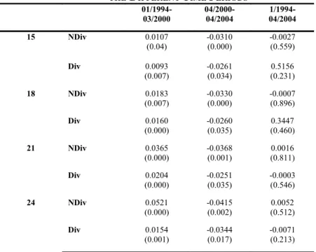
Table 6 presents the returns of the 6 -month ranking period strategy up to 24 months before and after the crash. Before the crash, all the returns are positive and statistically significant. First, these results prove the profitability of the momentum strategy in the long run for the two samples. Second, the significant momentum effect observed in the medium run in the non diversified sample continues to occur in the long run. The non -significant momentum effect recorded, in the medium run, in the diversified sample becomes significant in the long run. Third the momentum effect is more obvious for the non diversified sample. Finally, the returns of the trading strategies increase dramatically with the holding period in the long run.

TABLE6

RETURNS OF THE LONG TERM TRADING STRATEGIES IMPLEMENTED FOR THE DIFFERENT TIME PERIODS

01/1994-03/2000 04/2000-04/2004 04/2004 1/1994-15 NDiv 0.0107 (0.04) -0.0310 (0.000) -0.0027 (0.559) Div 0.0093 (0.007) -0.0261 (0.034) 0.5156 (0.231) 18 NDiv 0.0183 (0.007) -0.0330 (0.000) -0.0007 (0.896) Div 0.0160 (0.000) -0.0260 (0.035) 0.3447 (0.460) 21 NDiv 0.0365 (0.000) -0.0368 (0.001) 0.0016 (0.811) Div 0.0204 (0.000) -0.0251 (0.035) -0.0003 (0.546) 24 NDiv 0.0521 (0.000) -0.0415 (0.002) 0.0052 (0.512) Div 0.0154 (0.001) -0.0344(0.017) -0.0071(0.213) This table contains average returns to long term trading strategies implemented on the non diversified firms sample and the diversified firm sample and for different time period. The trading strategies buy winners and sell losers based on their past performance relative to the performance of an equal-weighted index of all stocks. The dollar profits are given by

it n it it =

∑

where ri,t is the return of stock i during the holding period t and the

investment weight assigned to stock i at time t is given by , *( ,1 1)

1 − − −       = it t t i r R N W , N is the total number of stocks in the sample, ri,t-1 is the return of stock i during the 6 month ranking

period t-1, Rt-1 is the average return across all stocks in the sample at time t-1 The numbers in

parentheses are significance level of realize profits of strategies.

After the crash, all the returns become negative and statistically significant. First, this evidence is in favour of the profitability of contrarian strategy in the long run for the two samples. In fact, the contrarian effect identified in the medium run continues to exist in the long run. Second, the contrarian effect become significant in the 6th

month for the diversified sample and in the 9th _{month for the non diversified sample. Third, the contrarian effect that}

was more important for the diversified sample in the medium run becomes more important for the non diversified sample in the long run. The reason is that, for the diversified sample, the return of the contrarian strategy is stabilized around 2,5% but for the non diversified sample, it grows more quickly and attains 4.1%. This implies that the diversified firms are more rapidly influenced by the crash but their prices are less affected.

5. Industrial diversification and the profitability of trading strategies: Alternative

explanations

5.1

The behavioral models have attempted to provide a framework for integrating predictability in stock returns. In this subsection, following Lee and Swaminathan (2000), we briefly summarize our results (Table 7) and discuss their relation to the behavioral models.

TABLE7

RESULTS’ SUMMARY: IMPACT OF THE INDUSTRIAL DIVERSIFICATION ON THE PROFITABILITY TRADING

STRATEGIES

Horizon 01/1994-03/2000 04/2000-04/2004 01/1994-04/2004

Sample

Medium run Momentum Effect Contrarian Effect Contrarian Effect

Long run Momentum Effect Contrarian Effect Contrarian Effect _{non significant}

Non -Diversified sub-sample

Medium run Momentum Effect Contrarian Effect_{( 9th month)} Momentum Effect _{non- significant}

Diversified sub-sample

Medium run Momentum Effect _{non significant} Contrarian Effect_{( 6th month)} Contrarian Effect

Long run Momentum Effect _{less pronounced} Contrarian Effect_{less pronounced} Contrarian Effect_{non significant}

First, we have noted that the trading strategies implemented on the non diversified sample do not earn significant returns and they earn negative returns when implemented on the diversified sample in the medium run. In the long run, however, all the trading strategies do not generate significant returns for the two samples. These outcomes seem to be driven by the important variability of the return before and after the March 2000 crash. So, we split our sample period at this date. We have found that, before the crash, the significant momentum effect observed in the medium run in the non diversified sample continues to exist in the long run. The non significant momentum effect recorded, in the medium run, in the diversified sample becomes significant in the long run. Nevertheless, the momentum effect is more pronounced for the non diversified sample. After the crash, only a contrarian effect is identified for both samples in both the medium and long run but it is more important for the non diversified sample.

Daniel et al. (1998) argue that stocks that are more difficult to value tend to generate greater overconfidence among investors. Therefore mispricing should be more severe among securities that are hard to value. If diversified firms tend to be difficult to value, then Daniel et al. (1998) would predict that return’s anomalies should be stronger among these firms. This is inconsistent with our finding that both before and after the crash mispricing is more pronounced among non diversified firms. The Hong and Stein (1999) model predicts that momentum profits should be larger for stocks with slower information diffusion2_{. If the following diversified firms}

require more resources and skills, these firms suffer from insufficient spread of information. If this is the case, the Hong and Stein model predict greater mispricing among these firms. Likewise, owing to less public information available about these stocks, one might expect relatively more private information to be produced. The Daniel et al. (1998) model suggests that mispricing is more severe among these stocks. Our results revealed this to be true among non diversified samples. Thus, our results fit with the hypothesis implying that corporate diversification is associated with a reduction in asymmetric information. Investor’s previsions about diversified firms seem to be less biased. A plausible explanation is that the errors that outsiders make in the forecasting segment cash flows are not perfectly positively- correlated so that the consolidated forecast is more accurate for a diversified than the forecast for a focused firm. Therefore, the price of the diversified firms diverge less from their fundamental value.

Nevertheless, the behavioral models predict a medium- horizon momentum -effect that reverse in the long horizon. Like Jegadeesh and Titman (2001), we found no evidence of reversals of the momentum effect in the 1990s (prior to the crash). After the crash, we identify only a contrarian effect and we find no evidence of momentum. This result corroborates recent works implying that the momentum strategies are not profitable. Shiller (2000), Campbell (2004) report that in the last twenty years simple momentum strategies have performed well on average, but in the period 2000-2003, these strategies performed relatively poorly. This may be accounted for by the widespread use of this strategy.

5.2

The momentum (contrarian) profits may be brought about by a cross-sectional dispersion in the expected stock returns rather than to their time series patterns. According to Conrad and Kaul(1998), purchasing past winners may imply a long position on high-risk stocks that earn higher expected returns. Inversely, selling past losers entails a short position on low-risk stocks that earn lower expected returns. Since the standard models like CAPM or the three-factor model fail to account for the cross-section of expected returns, the bootstrap simulation with replacement was proposed by Conrad and Kaul (1998). This technique allows to eliminate any time series’ properties in each security’s returns while maintaining the cross-sectional distribution of its mean returns; However, Jegadeesh and Titman (2002) show that the bootstrap with replacement introduce a small sample bias and they recommend the use of the bootstrap simulation without replacement. This bootstrap experiment consists in re-sampling without replacement, for each stock’s actual monthly returns: We generate 500 random samples by drawing without replacement the monthly returns. On each random sample, called bootstrapped sample, we implement the WRSS strategy.

Table 8 contains the average actual and average simulated profits of the 6-month ranking period strategies implemented on the diversified and the non -diversified samples. The holding periods range from six to 24 months. Panel A presents results for the 01/94-03/2000 time period and panel B presents results for the 01/94-04/2004. The first column (1) of each panel displays the average actual profit. The second column of each panel, presents the average simulated profits The simulated profit is an average of the 500 simulated returns yielded from the bootstrap without replacement with 500 replications. The third column presents percentage of simulated profit in actual profit.

TABLE8

AVERAGE PROFIT OF THEACTUAL AND SIMULATED TRADING STRATEGIES

Pannel A 01/94-03/2000 Pannel B 01/94-04/2004 (1) Actual profit (2) Simulate d profit (3) Percentag e (1) Actual profit (2) Simulate d profit (3) Percentag e 6 NDiv 0.0060*** 0.0040 66.67 0.0024 -0.0008 -33.33 Div 0.0008 0.0005 62.50 -0.0085* -0.0009 10.59 9 NDiv 0.0079** 0.0059 74.68 0.0001 -0.0011 -100.00 Div 0.0042 0.0015 35.71 -0.0144** -0.0016 11.11 12 NDiv 0.0111** 0.0077 69.37 -0.0023 -0.0020 86.96 Div -0.0092 0.0019 -20.65 -0.0138* -0.0021 15.22 18 NDiv 0.0183*** 0.0111 60.66 -0.0007 -0.0020 285.71 Div 0.0160*** 0.0043 26.88 0.3447 -0.0032 -0.93 24 NDiv 0.0521*** 0.0135 25.91 0.0052 -0.0029 -55.77 Div 0.0154*** 0.0069 44.81 -0.0070 -0.0043 61.43

This table contains average actual and average simulated profits to 6-month ranking period strategies implemented on the diversified sample and the non diversified sample. The holding periods range from 6 to 24 months. Pannel A presents results for the 01/94-03/2000 time period and the pannel B presents results for the 01/94-04/2004. The column (1) of each panel display average actual profit. The column, (2) of each panel, presents average simulated profits. The simulated profit is an average of the 500 si m u l ate d retur ns obtained from the bootstrap without replacement with 500 replications. The column (3) presents percentage of simulated profit in actual profit (percentage)

*Significant at 10% level **Significant at 5% ***Significant at 1%

Before the crash, the simulated profit of the non -diversified sample increases from 0.4% for the 6-month holding period strategy to 1.35% for the 24-month holding period strategy. However, the simulated profit of the diversified sample rises from 0.05% for the 6-month holding strategy to 0.69% for the 24-month holding strategy. This implies that the average simulated return goes up with the holding period but less than geometrically for the two samples. Second, the simulated returns of the diversified firms’ sample are lower than those of the non-diversified sample. The percentage of the simulated profit in actual profit is less than 100% for all the strategies and it doesn’t exceed 75% for the non diversified firm sample and 63% for the diversified firm sample. Therefore, the cross-sectional difference in expected returns does not, utterly, explain trad the ing strategies’ profits. By expanding the time period to 2004, the results indicate that only for the diversified sample, a contrarian strategy generates significant profits. The simulated profit of this strategy does not exceed 15.5%3_.

6. Conclusion

Prior studies affirm that industrial diversification has an impact on the level of information asymmetry. The behavioral models also suggest that momentum anomaly is affected by information asymmetry. Thus, the purpose of this paper is to analyze the impact of industrial diversification on the profitability of contrarian and momentum strategies. Using Monthly returns, the WRSS strategy is applied to 249 American listed stocks from January1,994 to April ,2004. Unlike the previous studies, which used older data, our findings reveal that the momentum strategy seems to stop being profitable. In order to study the impact of the 2000 crash on our results, we implemented the WRSS strategy during the [01/1994-03/2000] and the [04/2000-04/2004] sub-periods. Our results indicate that while momentum strategies earn large positive and significant returns during the first sub-period, these returns are negative during the second sub- period. As Hong and Stein (2003) report, the 2000 market crash is qualified by negative returns.

The stocks are divided into two groups according to the intensity of their industrial diversification using Ward (1963) method of hierarchical classification. Our results entail that the trading strategies implemented on the non -diversified sample do not earn significant returns but earn negative returns when implemented on the diversified sample in the medium run. In the long run, however, all the trading strategies do not generate significant returns for the two samples. These results seem to be driven by the great variability of return before and after the of March 2000 crash. In fact, we find that, before the crash, the significant momentum effect observed in the medium run in the non diversified sample continues to occur in the long run. The non -significant momentum effect recorded, in medium run, in the diversified sample becomes significant in the long run. Nevertheless, the momentum effect is more pronounced for the non diversified sample. After the crash, only a contrarian effect is identified for both samples in medium and long run but it is more important for the non diversified sample. We then try to explain these results with the predictions of several behavioral models. Like Lee and Swaminathan (2000), we conclude that each model has specific features that help explain some aspects of our findings but that no single model accommodates all our findings. Then, the Bootstrap without replacement is used to explore the risk- based explanation of the profitability of the trading strategies. We find that the cross-sectional differences in expected returns do not, entirely, account for the trading strategies’ profits.

B

Barberis N, Shleifer A. and Vishny R. A model of investor sentiment. Journal of Financial Economics1998; 49; 307–343.